Schloegl’s second model for autocatalysis on hypercubic lattices: Dimension dependence of generic two phase coexistence

Physics and Astronomy Publications

Physics and Astronomy

2012

Schloegl’s second model for autocatalysis on

hypercubic lattices: Dimension dependence of

generic two-phase coexistence

Chi-Jen Wang

Da-Jiang Liu

Ames Laboratory, [email protected]

James W. Evans

Iowa State University, [email protected]

Follow this and additional works at:

http://lib.dr.iastate.edu/physastro_pubs

Part of the

Mathematics Commons

, and the

Physics Commons

The complete bibliographic information for this item can be found athttp://lib.dr.iastate.edu/physastro_pubs/184. For information on how to cite this item, please visithttp://lib.dr.iastate.edu/howtocite.html.

Schloegl’s second model for autocatalysis on hypercubic lattices:

Dimension dependence of generic two-phase coexistence

Abstract

Schloegl's second model on a (d ≥ 2)-dimensional hypercubic lattice involves: (i) spontaneous annihilation of

particles with rate p and (ii) autocatalytic creation of particles at vacant sites at a rate proportional to the

number of suitable pairs of neighboring particles. This model provides a prototype for nonequilibrium

discontinuous phase transitions. However, it also exhibits nontrivial generic two-phase coexistence: Stable

populated and vacuum states coexist for a finite range, pf(d)

Keywords

autocatalytic, hypercubic lattices, interface dynamic, kinetic monte carlo simulation, master equations, non

equilibrium, planar interface, propagation failure, reaction diffusion equations, spinodals, stationary points,

vacant sites, Monte Carlo methods

Disciplines

Mathematics | Physics

Comments

This article is from

Physical Review E

85 (2012): 041109, doi:

10.1103/PhysRevE.85.041109

. Posted with

permission.

PHYSICAL REVIEW E85, 041109 (2012)

Schloegl’s second model for autocatalysis on hypercubic lattices:

Dimension dependence of generic two-phase coexistence

Chi-Jen Wang,1,2Da-Jiang Liu,1and J. W. Evans1,2,3

1_{Ames Laboratory, USDOE, Iowa State University, Ames, Iowa 50011, USA}

2_{Department of Mathematics, Iowa State University, Ames, Iowa 50011, USA}

3_{Department of Physics and Astronomy, Iowa State University, Ames, Iowa 50011, USA}

(Received 10 August 2011; published 9 April 2012)

Schloegl’s second model on a (d2)-dimensional hypercubic lattice involves: (i) spontaneous annihilation of particles with ratepand (ii) autocatalytic creation of particles at vacant sites at a rate proportional to the number of suitable pairs of neighboring particles. This model provides a prototype for nonequilibrium discontinuous phase transitions. However, it also exhibits nontrivial generic two-phase coexistence: Stable populated and vacuum states coexist for a finite range,pf(d)< p < pe(d),spanned by the orientation-dependent stationary points for planar interfaces separating these states. Analysis of interface dynamics from kinetic Monte Carlo simulation and from discrete reaction-diffusion equations (dRDEs) obtained from truncation of the exact master equation, reveals thatpe(f)∼0.211 3765+ce(f)/dasd→ ∞,wherec=ce−cf ≈0.014. A metastable populated state persists abovepe(d) up to a spinodalp=ps(d), which has a well-defined limitps(d→ ∞)= 1₄. The dRDEs display artificial propagation failure, absent in the stochastic model due to fluctuations. This feature is amplified for increasingd, thus complicating our analysis.

DOI:10.1103/PhysRevE.85.041109 PACS number(s): 05.70.Fh, 02.50.Ey, 05.45.−a, 05.50.+q

I. INTRODUCTION

Stochastic lattice-gas reaction and reaction-diffusion mod-els prescribe kinetic rules and rates for the creation and annihilation of various species residing on a lattice [1,2]. The reaction steps are often cooperative and are sometimes irreversible. The lack of a detailed-balance condition on the governing rates means that these systems may evolve to nonequilibrium steady states which are not characterized by a Gibbs measure familiar for thermodynamic equilibrium in Hamiltonian models. However, these steady states can display phase transitions somewhat analogous to those in thermodynamic systems [1,2]. For both equilibrium [3] and nonequilibrium [1] lattice-gas models, it can be instructive to consider behavior as a function of lattice dimension d. For models exhibiting continuous transitions or criticality, an upper critical dimension exists above which fluctuations are weak and mean-field (MF) behavior applies [1,3]. One also expects that either equilibrium or nonequilibrium discontinu-ous transitions may be erased due to strong fluctuations below some criticald =d∗[1–3].

A candidate for nonequilibrium discontinuous transitions is Schloegl’s second model for autocatalysis [4–13] on a hypercubic lattice which involves: (i) spontaneous annihilation of particlesXat occupied sites at ratepand (ii) autocatalytic creation of particles at vacant sites ø induced by suitable nearby pairs of particles [8–13]. Schematically, the reaction steps are as follows:

X→o/ (spontaneous annihilation at ratep), o

/+2X→3X (autocatalytic creation).

MF analysis suggests the existence of a discontinuous transition between an active state with particle concentration C >0 for 0< p < peand an absorbing vacuum stateC=0 for allp >0. However, kinetic Monte Carlo (KMC) analysis of Grassberger’s version of this model found only a continuous

transition for d <4, suggesting a critical d∗ = 4 [5]. In contrast, our KMC analysis for a version of the model based on Durrett’s Quadratic Contact Process (QCP) (see below) revealed a discontinuous transition ford=2 [9] andd=3 [13], suggesting thatd∗=2.

In addition, our analysis of the QCP version revealed a

nontrivial generic two-phase coexistence (2PC) for d = 2 andd =3 wherein the stable populated and vacuum phases coexist for a finite range of annihilation ratep[9–13]. (Trivial

2PC occurs due to a “quirk” in the QCP rules. For any p > 0, the vacuum state can always resist the growth of active droplets which cannot escape any rectangular region containing them [8]. Trivial 2PC disappears upon perturbing the model, e.g., to include particle hopping or spontaneous creation.) The nontrivial 2PC derives from an orientation dependence of the value of the annihilation rate p = peq, corresponding to a stationary planar interface separating the two phases. This nontrivial generic 2PC feature may persist for d > 3. This behavior contrasts phase coexistence in an equilibrium Hamiltonian system where planar interface separating phases is stationary at a unique point, corresponding to equality of chemical potentials. As an aside, generic 2PC was explored in Toom’s model for voter dynamics [14,15] where the kinetic rules have an unappealing [16] asymmetry.

Our goal here is to elucidate fundamental aspects of the dependence on dimension d of discontinuous transitions in lattice-gas reaction models which display generic 2PC. In this paper, we consider only our QCP version of Schloegl’s second model, but the features displayed and issues analyzed will undoubtedly have broad applicability. Analogous stud-ies for equilibrium systems would be performed using the ferromagnetic Ising model. One might expect the kinetics to approach mean-field behavior, and enhanced metastability as d → ∞. However, the d dependence of features related to equistability of distinct phases is perhaps less clear and is the

041109-1

CHI-JEN WANG, DA-JIANG LIU, AND J. W. EVANS PHYSICAL REVIEW E85, 041109 (2012)

focus of the current paper. Although contentious [17], we claim that equistability for infinite lattices should be determined by stationarity of planar interfaces separating coexisting states (cf. Refs. [4,18–22]). Consideration of equistability is complicated by the presence of generic 2PC for which we provide an analysis of its d dependence and disappearance asd → ∞.

With regard to development and application of general methodologies, we apply discrete reaction-diffusion equations (dRDEs) to elucidate interface dynamics. dRDEs are derived from truncation approximations to the exact master equations for spatially inhomogeneous states. This approach previously has received little attention, and then only for d = 1–3 and mainly using the lowest-order mean-field truncation approximation. We exploit the dRDEs to obtain exact limiting behavior asd → ∞. However, we find that these dRDEs can display artificial propagation failure (APF), an effect which is absent due to fluctuations in the stochastic model and which is strongly amplified with increasingd. Nonetheless, dRDE analysis of suitable interface orientations avoiding APF is shown to still capture behavior in the stochastic model. While we treat only our QCP model, this dRDE methodology and the observed APF behavior and its resolution should have broad applicability.

In Sec. II, we provide a detailed description of our stochastic reaction model for general d 2. KMC simulation results are reported for d = 2–5. In Sec. III, we present the exact master equations for general d and develop dRDEs for spatially heterogeneous states by applying the MF and pair approximations in Sec. IV. The dRDEs are used to assess the propagation of planar interfaces between active and vacuum states, specifically stationarity and APF in Sec. V. The interpretation of the dRDE results and their relationship to exact behavior of the stochastic reaction model is described in Sec. VI. Conclusions are provided in Sec. VII.

II. MODEL PRESCRIPTION FOR GENERAL DIMENSION AND KMC ANALYSIS

Our model involves particle annihilation and creation at the sites of an infinited-dimensional hypercubic lattice with sites labeled byi=(i1,i2,i3, . . . ,id). Note that the total number of pairs of sites selected from the 2d nearest neighbors (NNs) of any site satisfiesktot =(2d)(2d − 1)/2! =d(2d − 1).

We divide all such pairs into two subsets: linear pairs where one site is (i₁,i₂, . . . ,ij +1, . . . ,id) and the other is (i₁,i₂, . . . ,ij −1, . . . ,id) and “diagonal” pairs where one site is at one of (i1,i2, . . . ,ij ±1,id) and another is at one of (i1,i2, . . . ,ik±1, . . . ,id) and where j = k. The number of linear pairs satisfies klin = d, and thus, the number of

diagonal pairs satisfies kmax = ktot − klin = 2d(d − 1).

Our QCP version of Schloegl’s second model for any d 2 generalizes Durrett’s prescription [8] for a d = 2. It involves: (i) spontaneous creation of particles at unoccupied sites at ratep and (ii) autocatalytic annihilation of particles at empty sites at rate k/kmax, where k is the number

of diagonal pairs of particles on neighboring sites. This prescription produces a simple d-independent form for the mean-field kinetics of the model. Furthermore, it enables an

exact simplification of the master equations as described in Sec. III.

For spatially homogeneous states, we define the particle concentrationCas the mean probability that a site is occupied so that 0C1. We find that a stable populated steady state with concentrationC >0 exists for a range of annihilation rates 0 p pe(d). Previous KMC papers found pe(d =2) = 0.094 43 [9] and pe(d = 3) = 0.139 39 [13]. Below, we report behavior for d > 3. In the “active” populated state, particles are continually created and annihilated. Increasingp to higherp > pe(d) results in a discontinuous transition to a stable absorbing “vacuum” state with C =0. An ill-defined metastable extension of the active state exists for a small range ofpe(d)< p < ps(d), whereps(d) denotes the spinodal with ps(d=2)≈0.101 [12] andps(d=3)≈0.15 [13].

Previous papers ford = 2 and 3 [9,12] found nontrivial generic 2PC wherein stable active and vacuum states coexist for a finite rangepf(d)ppe(d). This range is spanned by the orientation-dependent “equistability” valuesp =peq for stationary planar interfaces separating these states, where pe(d)=maxpeq corresponds to a diagonal (d =2) or skew (d=3) interface. For a general orientation, when 0p < peq, the active state displaces the vacuum state. Forpeq<p<pe(d), the vacuum state displaces the active state. Forpe(d)< p < ps, the vacuum state transiently displaces the metastable active state until the latter spontaneously converts to the vacuum. One caveat is that, for an exactly vertical interface (i₁=0), the active state can never propagate into the vacuum (empty sites in this vacuum state have, at most, one occupied neighbor). More precisely, a vertical interface is stationary for allppf(d), but the vacuum state expands forp > pf(d). See Refs. [9–13] and Fig.1. As noted above, trivial 2PC occurs for allp pe(d) as the vacuum state is stable against expansion of droplets of the active state. These features are shown to persist for d >3.

Model behavior is characterized by performing KMC simulations on finite hypercubic lattices of Ld _{sites with} periodic boundary conditions. In conventional constant-p ensemble simulations, processes are implemented with prob-abilities proportional to their rates. However, to assess peq, we implement alternative constant-C ensemble simulations [9,23]. System sizes were typicallyL =1024, 128, 48, and 20, ford=2–5, respectively. Simulation data were collected over times∼106_{Monte Carlo steps (MCS) ford =2–4 and}

∼104MCS ford=5.

For d 2 dimensions, the interface orientation where ai1+bi2+ci3+ · · · =m is constant (with a,b, c,. . ., and

m as integers) is labeled by (abc· · ·). Vertical interfaces correspond to a = 1 and b=c= · · · =0 (so i₁ = m) are (10), (100), (1000), etc., ford =2,3,4,. . ., respectively, and have peq(d) =pf(d) defined as the upper boundary of the region of propagation failure 0 < p < pf(d). We define a “hyperskew” (HS) orientation as that where a =b=c=

· · · =1 (soi₁+i₂+i₃+ · · · +id =m) which constitutes the furthest-from-vertical orientation. This hyperskew orienta-tion corresponds to diagonal (11), skew (111), fourth-order skew (1111),. . ., for d = 2,3,4,. . ., respectively, and has peq(d)=pe(d), i.e.,peq is highest for orientations furthest from vertical where the active state can most easily displace the vacuum state. Results forpeq(d =2–5) for various interface

SCHLOEGL’s SECOND MODEL FOR AUTOCATALYSIS ON. . . PHYSICAL REVIEW E85, 041109 (2012)

(a) (b)

FIG. 1. (Color online) Steady-state C versus p for (a)d=2; (b) d → ∞ MF behavior. pe (pf)=upper (lower) 2PC boundaries;

ps=spinodal. Inset to (a), dependence of equistabilitypeqon interface orientation. Inset to (b), profile of a hyperskew interface ford→ ∞at

pe=pf =0.211 3765.

orientations are shown in TableI. In Sec. V, we show that peq(d → ∞) = 0.211 3765 for all orientations. Our data suggest thatpeq(d)≈peq(d → ∞)+c/d, wherecdepends weakly on orientation. See Fig.2. The width of the 2PC region satisfiespeq(d)=pe(d)−pf(d)≈0.014/d.

III. MASTER EQUATIONS FOR HOMOGENEOUS AND INHOMOGENEOUS STATES

Letx(o) denote a filled (empty) site, and let P’s denote the probabilities for various configurations of clusters of sites. For general spatially inhomogeneous states, the probability that a site is occupied or is vacant depends on its location. Thus, we let Ci = P[xi] denote the probability that site

i =(i1,i2, . . . , id) is occupied. Then, P[oi] = 1 − P[xi]

is the probability that sitei is empty. Let e1 = (1,0,0,. . .),

e2=(0,1,0,. . .), etc., denote vectors between NN sites. Then,

P[xi xi+e1](P[oi oi+e1]) denotes the probability that sites

in the NN pair i,i + e1 are both occupied (empty). Also,

P[xi oi+e1] andP[oi xi+e1] denote the probabilities of mixed

occupied-empty pairs. Conservation of probability implies that P[xi] + P[oi] = 1, P[xi oi₊e1]+P[xi xi₊e1]=

P[xi],P[oi xi+e1]+P[oi oi+e1]=P[oi], etc. For the

spe-cial case of spatially homogeneous states, these quanti-ties do not depend on site location, so P[xi]=P[x]=C,

P[oi]=P[o]=1 − C (=C), etc. The exact master

equa-tions for our reaction model can be written as a cou-pled hierarchy for the evolution of the probabilities for empty single sites, empty pairs, etc. [24]. Terms in these equations simply account for all possible gain pathways due to spontaneous particle annihilation and all possi-ble loss pathways associated with autocatalytic particle creation.

A. Lowest-order hierarchical equation for single-site probabilities

For spatially inhomogeneous states, the equations for single empty sites have the exact form

d/dt P[oi]=pP[xi]−(1/kmax){P[oi xi₊e1 xi₊e2]

+P[oi xi+e1 xi−e2]+P[oi xi+e1 xi+e3]+ · · ·}

(1)

The first gain term on the right-hand side (RHS) of Eq.(1)

corresponds to spontaneous particle annihilation at siteiat rate p. The other loss terms correspond to autocatalytic particle creation at empty sitei where one term appears for each of thek_maxpossible configurations of diagonal pairs of particles on sites NN toi. We have shown explicitly only three out of thesekmax creation terms. From Eq.(1), it is clear that, for

a spatially homogeneous state, the evolution equation for the probability of a single empty site has thed-independent exact form

d/dt P[o]=pP[x]−Px_{o x}. (2)

The loss term on the right-hand side denotes the probability of a filled site with a specific diagonal pair of filled sites, where the state of the 2d − 2 other neighboring sites is unspecified. In deriving the loss terms in Eq.(1),P[oi xi+e1 xi+e2]

cor-responds to a sum of contributions for different configurations of the 2d sites surrounding oi but all including a diagonal

pair of particles at sites i + e1 and i + e2. One case is

the configuration with all other 2d − 2 neighboring sites empty, so k=1, associated with a creation rate of 1/kmax.

The general case has k − 1 additional diagonal pairs with creation rate k/kmax. We associate a fraction 1/k of this

contribution with the term P[oi xi₊e1 xi₊e2], and the rest

is equally distributed between the other terms. Summing all

TABLE I. KMC values ofp=peqfor stationary planar interfaces separating populated and vacuum states for orientations indicated before the colon;peq→0.211 377 asd→ ∞for all orientations.

d=2 10:0.0871 11:0.094 40 (2)

d=3 100:0.1353 110:0.139 027(7) 111:0.139 386(7)

d=4 1000:0.1548 1100:0.157 593(9) 1110:0.158 091(8) 1111:0.158 284(8)

d=5 10 000:0.1664 11 000:0.168 24(1) 11 100:0.168 847(7) 11 110:0.169 055(6) 11 111:0.169 137(6)

CHI-JEN WANG, DA-JIANG LIU, AND J. W. EVANS PHYSICAL REVIEW E85, 041109 (2012)

FIG. 2. KMC results forpeq versus 1/d for hyperskew (filled square) and vertical (open square) interfaces where the exact result is also shown ford→ ∞.

contributions associated withP[oi xi+e1 xi+e2], thus, yields

1/kmax times the probability that site i is empty, and the

indicated diagonal pair is occupied (with all other neighbors of the empty site in an unspecified state). A similar analysis generatesP[oi xi₊e1 xi₋e2] and the other terms.

For spatially inhomogeneous states corresponding to planar interfaces between populated and vacuum states, Eq. (1)

adopts a simpler form. For specific orientations, theCi1,i2,...,id and related probabilities can be independent of some ik or dependent only on certain combinations of them. Also, some probabilities for configurations of clusters of sites become identical. For example, for vertical interfaces where Ci1,i2,...,id=Ci1, the first two particle creation terms in Eq.(1)

are equivalent.

B. Hierarchical equation for pair probabilities

One can also obtain equations for probabilities of adjacent empty pairs of sites and for larger clusters of empty sites. For a spatially inhomogeneous state, the evolution equation for the pair probabilityP[oi oi+e1] has the exact form

d/dt P[oioi₊e1]

=p{P[xioi+e1]+P[oixi+e1]} −(1/kmax)

× {P[oioi+e1xi+2e1xi+e1+e2]+ · · ·}

−(1/kmax){P[xi₊e2xi₋e1oioi₊e1]+ · · ·}. (3)

The first two gain terms on the RHS correspond to spontaneous particle annihilation at siteiandi + e1 at rate

p. The next group of loss terms corresponds to autocatalytic particle creation at empty sitei + e1where one term appears

for each of the 2(d − 1) possible configurations of diagonal pairs of particle NNs for this site, where neither particle is on the neighboring sitei. We have shown explicitly only one out of the subset of 2(d − 1) configurations where one particle forms a linear triple with the empty pair. There is another larger subset of 2(d −1)(d −2) configurations where neither particle forms a linear triple with the empty pair. The analogous last group of loss terms corresponds to autocatalytic particle creation at empty siteiwhere one term appears for each of the total of 2(d −1)2_{possible configurations of diagonal pairs of}

particle NNs for this site.

From Eq.(3), it follows that, for a spatially homogeneous state, the equation for evolution of the probability of an empty pair has the exact form

d/dt P[o o]=2pP[x o]− {4(d−1)/kmax}P

_x

o o x

− {4(d−1)(d−2)/kmax}P

_x

o ⊗

, (4)

whereP[_{o o x}x ] andP[_{o ⊗}x] represent probabilities of an empty pair where the right site in this pair has a diagonal neighboring pair of particles. In the first, one filled site forms a linear triple with the empty pair. In the second, both filled sites form bent triples with the empty pair.

Derivation of the loss terms in Eq.(3)due to autocatalytic particle creation follows a similar strategy as that for Eq.(1)

above. Each term corresponds to a sum of contributions associated with different configurations of the 2d − 1 sites at the relevant end of the empty pair [oi oi₊e1] but which

all include the diagonal pair of particles indicated explicitly in Eq.(3). Summing all contributions associated with the specific pair, thus, yields 1/kmax times the probability that the pair is

empty, and the specific diagonal pair is occupied (with other neighbors of the empty pair unspecified).

IV. APPROXIMATIONS AND DISCRETE REACTION-DIFFUSION EQUATIONS

A. Truncation approximations

In the simplest MF or site approximation, one neglects all correlations in the occupancy of different sites. Thus, for example, one has that

P[oi xi₊e1 xi₊e2]

≈ P[oi]P[xi₊e1]P[xi₊e2]

reducing toPx_{o x}≈P[o]P[x]2 (5) for inhomogeneous (homogeneous) states. In the next higher-order pair approximation, probability configurations of clus-ters of sites are factorized in terms of those for all constituent pairs where one also compensates for double counting of some sites. Thus, one has that

P[oixi₊e1xi₊e2]≈P[oixi₊e1]P[oixi₊e2]/P[oi]

and P[oioi+e1xi+2e1xi+e1+e2]

≈P[oioi+e1]P[oi+e1xi+2e1]

×P[oi₊e1xi₊e1+e2]/P[oi₊e1]2 (6)

(reducing toP[x_{o x}]≈P[x o_]2/P[o] andP[_ooxx ]≈P[_{o ⊗}x]≈ P[o o_]P[x o_]2/P[o]2), for inhomogeneous (homogenous) states.

B. Mean-field type kinetics for homogeneous states

The MF site approximation for Eq. (2) yields the d -independent MF kinetics,

d/dt C= −pC+C2(1−C)≡R(C), sod/dt lnC=(C/C)[p−CC], (7)

SCHLOEGL’s SECOND MODEL FOR AUTOCATALYSIS ON. . . PHYSICAL REVIEW E85, 041109 (2012)

where C=1 − C gives the probability of an empty site. Steady-state analysis reveals a stable vacuum state with C=0 for all p > 0 and a stable active state with C=Cact(MF)= 1₂+₂1(1−4p)1/2 for a bistability regime 0pps(MF)=1₄ [4,8–10]. In the pair approximation, a natural variable is the conditional concentration, K= P[x o]/P[o],representing the probability of finding a particle next to a site specified empty. Setting K=1 − K (the conditional probability of an empty site) andcd=(d − 1)/d, the pair kinetics can be instructively formulated as

d/dtlnC=(C/C)[p−CC(K/C)2]

and d/dtlnK+d/dtlnC=2(K/K)[p−cdKK]. (8)

A steady-state analysis yields a stable vacuum state with C=K=0 for all p > 0, and a stable active state K= K_act(pair)=1₂ +1₂(1−4p/cd)1/2for a bistability regime 0 p ps(pair)=cd/4. Since cd → 1 as d → ∞, it is clear comparing Eqs.(7)and(8)that site and pair approximations converge.

More generally, consider the evolution of the probability P[{o}n] of a finite connected cluster ofnvacant sites{o}n. The key observation is that, asd→ ∞, all sites are on the perimeter and almost fully coordinated with sites not in the cluster. More precisely, the fractional deficit from full coordination scales, such as 1/d. Thus, the structure of the evolution equation is similar to that for the probability (P[o])n _{forn isolated} far-separated sites. It follows thatP[{o}n]→(P[o])nasd→ ∞, a general feature, applying for any lattice-gas reaction model.

C. Mean-field-type dRDE

We will consider only spatially inhomogeneous states corresponding to planar interfaces between active and vacuum states. As in Sec. II, interface orientations whereai₁+bi₂+ ci₃+ · · · =mis constant are labeled by (abc· · ·) ford 2 dimensions. In these cases, the concentrations Ci1,i2,...,id = Cai1+bi2+ci3···=m=Cm are labeled by a single integer m. Applying MF factorization to Eq. (1) produces dRDE-type equations for theCm. The “diffusion”-type terms reflect spatial coupling in the reaction model rather than particle hopping. These types of MF dRDEs have been explored previously for other reaction-diffusion models, but only for d 3 [25–27]. It is convenient to define a pseudodiffusion coefficient Dj(C)=C(1 − C)/jand the discrete Laplacian,

Cm=Cm₊1−2Cm+Cm₋1 so that

(Cm+1+Cm−1)2−(2Cm)2=4CmCm+(Cm)2. (9) For hyperskew (1111· · ·) interfaces where Ci1,i2,...,id = Ci1+i2+···+id=m, one obtains the MF dRDEs,

d/dt Cm= −pCm+1₄(1−Cm)(Cm+1+Cm−1)2

=R(Cm)+D1(Cm)Cm

+1

4(1−Cm)(Cm+1+Cm−1)

2_{, (10)}

which have a form independent ofd. As a consequence, the MF value ofpeq for thed=2 diagonal,d=3 skew, andd > 3 hyperskew orientations will be identical. It should be noted that the physical Euclidean distance between adjacent planes mandm + 1 equalsd−1/2, and thus, the physical width of

(a) (b)

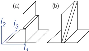
FIG. 3. (Color online) Schematic ford=3 of (a) a rare horizontal and (b) a hyperskew step on a vertical interface.

the concentration profile across the interface also scales like d−1/2_.

For vertical (1000· · ·) interfaces whereCi1,i2,...,id=Ci1=m, one obtains the distinct MF dRDE,

d/dt Cm=R(Cm)+Dd(Cm)Cm, (11)

incorporating weak spatial coupling for largeddue to smallDd

∼1/d. SinceR(0)=0 andDd(0)=0, Eq.(11)appropriately ensures that the active state cannot displace the vacuum state. Next, consider more general low-index interfaces including diagonal (11 000· · ·) interfaces whereCi1,i2,...,id=Ci1+i2=m, skew (11 100· · ·) interfaces Ci1,i2,...,id =Ci1+i2+i3=m, and the natural generalization tonth-order skew interfaces where Ci1,i2,...,id=Ci1+i2+i3+···+in=m. For the general nth-order skew case, one obtains the MF RDE,

d/dt Cm=R(Cm)+nDd(Cm)Cm

+1

4n(n−1)d−

1_(d−1)−1_(C

m)2. (12) This result includes vertical (n=1), diagonal (n=2), and skew (n=3) orientations as special cases and reveals weak spatial coupling in all cases with n=O(1) and large d in contrast to Eq.(10).

For reasons discussed below, it will also be instructive to consider near-vertical orientations. When Si1 +i2=m,

corresponding to a near-vertical interface with large slopeS and far-spaced rare “horizontal steps” [see Fig. 3(a)], one obtains the MF dRDE,

d/dt Cm = −pCm+d−1(d−1)−1(d−2)(d−3)

×(1−Cm)(Cm)2+d−1(d−1)−1(d−2)(1−Cm)

×Cm(Cm−1+Cm+1+Cm−S+Cm+S)

+1 2d−

1_(d−1)−1_(1−C

m)(Cm₋1+Cm₊1)

×(Cm−S+Cm+S). (13) When Si₁+i₂+ · · · +id =m, corresponding to a near-vertical interface with large slope S and far-spaced rare “maximally kinked” or hyperskew steps [see Fig. 3(b)], one obtains the MF dRDE,

d/dt Cm = −pCm+1₄d−1(d−2)(1−Cm)(Cm−1+Cm+1)2

+1 2d−

1

(1−Cm)(Cm−1+Cm+1)(Cm−S+Cm+S). (14)

Writing Eqs.(13)and(14)in the formd/dt Cm=R(Cm) + “diffusion-type terms,” these diffusion terms are on the order of 1/din Eq.(13)but on the order of unity in Eq.(14)[which reduces to Eq.(10)asd→ ∞].

One can also apply the pair approximation to Eqs.(1)and

(3)for planar interfaces between active and vacuum states to

CHI-JEN WANG, DA-JIANG LIU, AND J. W. EVANS PHYSICAL REVIEW E85, 041109 (2012)

TABLE II. MF results for stationary pointsp=peq for regimes of propagation failure for planar interfaces separating populated and vacuum states. Results shown forS=1024.

Vertical Si1 Diagonal S(i1+i2) Skew S(i1+i2+i3) Hyperskew

1000· · · Si1+i2 +i2+ · · · +id 11 000· · · +i3+ · · · +id 11 100· · · +i4+ · · · +id 111· · ·

d=2 0.207 1068 0.205 051 0.211 3765

d=3 0.210 38 0.206 02 0.206 05 0.210 23–0.210 37 0.210 30 0.211 3765

d=4 0.215 14 0.207 20 0.207 32 0.209 49–0.210 27 0.209 90 0.210 93 0.210 92 0.211 3765

d=5 0.219 53 0.207 82–0.208 29 0.208 34 0.208 20–0.210 99 0.209 74 0.210 60–0.210 75 0.210 68 0.211 3765

d=6 0.223 12 0.207 17–0.209 74 0.209 06 0.205 83–0.212 46 0.209 71 0.210 24–0.210 81 0.210 53 0.211 3765

d=7 0.226 00 0.204 68–0.211 75 0.209 57 0.202 22–0.214 37 0.209 77 0.209 59–0.211 20 0.210 45 0.211 3765

d=10 0.231 88 0.188 16–0.218 45 0.210 39 0.185 59–0.220 35 0.210 15 0.204 96–0.214 14 0.210 39 0.211 3765

d=100 0.247 73 0.032 35–0.245 58 0.211 365 0.032 34–0.245 66 0.211 35 0.049 77–0.243 70 0.211 34 0.211 3765

d=1000 0.249 76 0.003 39–0.249 52 0.211 3764 0.003 40–0.249 52 0.211 3763 0.005 31–0.249 29 0.211 3762 0.211 3765

d= ∞ 0–0.25 0–0.25 0–0.25 0–0.25 0.211 3765

obtain pair dRDEs forCmand related pair probabilities. See Appendix A for the special cases of hyperskew (1111· · ·) and vertical (1000· · ·) interfaces.

V. dRDE ANALYSIS: MEAN-FIELD AND PAIR RESULTS

We now present results from numerical integration of the dRDEs for evolution of planar interfaces between the active and the vacuum states. The initial data are chosen as a sharp interface between the active stateCm=Cactform<m∗and the

vacuum stateCm=0 formm∗. In the pair approximation, we also specify certain pair occupations determined from Kact(pair). The interface location is determined from m =

mCm/Cact for a large finite system of ∼1000 sites. The

interface velocity V(p)=d/dtm is determined for long times t ≈4 × 104_{. Our focus is on assessing variation in}

V(p) withpto determine stationarity and propagation failure.

A. Hyperskew (1111· · ·) orientation

The MF dRDEs for the hyperskew orientation where m=i1+i2+ · · · +id have the special feature of being independent of d. Analysis of interface propagation reveals thatV(p) vanishes at a single stationary point which has the d-independent MF valuepeq(111· · ·)=0.211 3765(4). See TableII. The pair dRDEs for the hyperskew orientation predict qualitatively similar interface evolution withV(p) vanishing

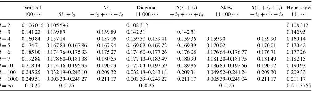
at a single stationary point. However, the pair peq(111· · ·) depends on dimension and increases smoothly to converge to the MF value asd→ ∞. See TableIII. Continuously deviating from a hyperskew orientation produces continuous deviations from the above behavior either at the MF or at the pair level withpeqshifting to lower values.

B. Vertical (1000· · ·) and near-vertical orientations

The MF dRDEs for vertical interfaces where m=i1

predict propagation failure for 0< p < peq(100· · ·) where MFpeq(100· · ·) increases withd. In fact, MFpeq(100· · ·)→ ps(MF)=1₄ asd → ∞where the interface is stationary over the entire bistability regime. See TableII. Additional analysis elucidates the sharpening of the stationary interface atp=peq asdincreases. See Appendix B. Analysis of the pair dRDEs, Eq. (A1), reveals the same qualitative behavior where the pairpeq(100· · ·)→ps(MF)=1₄ as d → ∞but the rate of convergence is slower. See TableIII.

1. Deviation from a vertical orientation with rare horizontal “steps” [cf. Fig.3(a)]

Both MF and pair analysis for near-vertical orientations with rare horizontal (H) steps (Si₁+i₂=m with large S =1024) indicates a unique stationary pointpeq(100· · ·H) for d=2–5, which shifts upward with d. For d 6, a finite range of propagation failure emerges over a

TABLE III. Pair approximation results for stationary pointsp=peqor for regimes of propagation failure for planar interfaces separating populated and vacuum states. Results shown forS=1024.

Vertical Si1 Diagonal S(i1+i2) Skew S(i1+i2+i3) Hyperskew

100· · · Si1+i2 +i2+ · · · +id 11 000· · · +i3+ · · · +id 11 100· · · +i4+ · · · +id 111· · ·

d=2 0.106 016 0.105 596 0.108 312 0.108 312

d=3 0.141 23 0.139 89 0.139 89 0.142 51 0.142 51 0.142 95

d=4 0.160 84 0.157 14 0.157 16 0.159 30–0.159 41 0.159 36 0.159 90 0.159 90 0.160 14

d=5 0.174 71 0.167 83–0.167 86 0.167 94 0.169 02–0.169 72 0.169 39 0.170 02 0.170 01 0.170 42

d=6 0.185 00 0.174 76–0.175 33 0.175 27 0.174 60–0.177 26 0.176 08 0.176 64–0.176 77 0.176 71 0.177 26

d=7 0.192 88 0.178 60–0.181 38 0.180 55 0.177 13–0.183 49 0.180 90 0.181 20–0.181 75 0.181 49 0.182 15

d=10 0.208 14 0.174 46–0.195 93 0.190 03 0.172 04–0.197 69 0.189 85 0.186 83–0.192 56 0.190 12 0.190 93

d=100 0.245 25 0.032 19–0.243 10 0.209 32 0.032 18–0.243 18 0.209 31 0.049 52–0.241 24 0.209 30 0.209 33

d=1000 0.249 51 0.003 39–0.249 27 0.211 17 0.003 39–0.249 27 0.211 17 0.005 39–0.249 04 0.211 17 0.211 17

d= ∞ 0–0.25 0–0.25 0–0.25 0–0.25 0.211 3765

SCHLOEGL’s SECOND MODEL FOR AUTOCATALYSIS ON. . . PHYSICAL REVIEW E85, 041109 (2012)

regimep₋(100· · ·H)< p < p₊(100· · ·H). This regime expands with increasing d to cover the entire region of bistability, i.e., p₋(100· · ·H)→0 andp₊(100· · ·H)→ ps(MF)= 1₄asd→ ∞. See TablesIIandIII.

2. Deviation from a vertical orientation with rare HS steps [cf. Fig.3(b)]

Orientations defined bySi1+i2+ · · · +id =mwith large S correspond to a vertical interface i₁=0 misoriented by occasional hyperskew (maximally kinked) steps separated by verticalS lattice constants. Analysis based on both the MF and the pair dRDEs forS=1024 indicates a unique stationary point for whichpeq(100· · ·H S)→limd_→∞peq(111· · ·)= 0.211 3765, asd → ∞. See TablesIIandIII.

C. Diagonal (11 000· · ·), skew(11 100· · ·), and other orientations

Analysis of the MF and pair dRDEs for diagonal (11 000· · ·) interfaces where m=i₁+i₂ reveals that, ex-cept for small d, one has propagation failure over a regime p₋(1100· · ·)< p < p₊(1100· · ·). The regime of propagation failure expands with increasing d to cover the entire region of bistability, i.e., p₋(1100· · ·)→0 andp₊(1100· · ·)→ps(MF)= 1₄ as d → ∞. See TablesII andIII. Motivated by the analysis of near-vertical interfaces, we also consider deviations from diagonal orientations as-sociated with rare hyperskew (maximally kinked) steps as a route to eliminate propagation failure. These orientations are described by S(i₁+i₂)+i₃+i₄+ · · · +id =m, where we chooseS=1024. Analysis for the MF and pair dRDEs reveals a lack of propagation failure with stationary point peq(1100· · ·H S)→limd→∞peq(111· · ·)=0.211 3765 as d→ ∞. See TablesIIandIII.

Analysis of both MF and pair dRDEs for skew (11 100· · ·) interfaces reveals that, except for smalld, one has propaga-tion failure over a regimep₋(1110· · ·)< p < p₊(1110· · ·). Again, the regime of propagation failure expands with in-creasing d to cover the entire region of bistability, i.e., p₋(1110· · ·)→0 andp₊(1110· · ·)→ps(MF)=1₄ asd →

∞. It is also the case that propagation failure can be eliminated by deviating from skew orientations with rare hyperskew steps. These orientations are described byS(i1+i2+i3)+

i4+ · · · +id =m where we choose S=1024. The sta-tionary point peq(1110· · ·H S)→limd_→∞peq(111· · ·)= 0.211 3765 asd→ ∞. See TablesIIandIII.

One can extend the above investigations to considern th-order skew orientations as defined in Sec. IV B. One anticipates analogous behavior, i.e., development of propagation failure with increasingd, which engulfs the entire bistable regime as d→ ∞. It is also anticipated that deviating from these orienta-tions with rare hyperskew steps eliminates propagation failure.

VI. RELATING dRDE PREDICTIONS TO STOCHASTIC MODEL BEHAVIOR

In relating MF-type dRDE predictions to stochastic reaction model behavior, it is instructive to first focus on two key interface orientations, hyperskew and vertical.

For hyperskew (111· · ·) interfaces, the correspondence is unambiguous: There is no propagation failure for MF or pair dRDEs, and the predicted peq(111· · ·) corresponds to that in the stochastic model. The large discrepancy between the d-independent MF predictions and the KMC values of peq(111· · ·) for smaller d is largely removed in the pair approximation. As noted previously, the simple form peq(111· · ·)≈0.211 3765+c/d describes well observedd dependence.

For vertical (100· · ·) interfaces, recall that propagation fail-ure is expected forpbelow some critical value,peq(1000· · ·) as the active state cannot displace the vacuum state for anyp 0. Forp > peq(1000· · ·), the vacuum state displaces the pop-ulated state. This feature applies to both the stochastic model and to the various MF-type dRDEs. However,peq(1000· · ·), from MF-type treatments, does not correspond to that for the stochastic model as estimated by KMC simulations. Specif-ically, MF-type formulations “artificially extend” the regime of propagation failure. This feature is amplified for increasing d, recalling that MF-type peq(1000· · ·)→ps(MF)=1₄ as d → ∞.

Artificial propagation failure (APF) in MF-type dRDE treatments can be understood as follows. For smooth vertical interfaces in the stochastic lattice-gas reaction model, propaga-tion of the vacuum state into the populated state forp > peqis associated with fluctuation-mediated nucleation and growth of (d −1)-dimensional droplets of the vacuum state in the layer adjacent to the completely empty edge layer of the vacuum state. This feature is not reflected in MF-type treatments where more difficult “spatially homogeneous propagation” of the vacuum state into the next layer is required.

Considering near-vertical interfaces in MF-type treatments, i.e., vertical interfaces with far-separated steps, could poten-tially avoid APF. However, introducing “smooth” horizontal steps does not avoid APF. Why? Step propagation in the MF dRDE must occur by spatially homogeneous propagation rather than by fluctuation-mediated nucleation and growth of new rows of empty sites adjacent to the step as in the stochastic reaction model. However, introducing more easily propagating maximally kinked hyperskew steps avoids APF.

The amplification of APF with increasingd follows from the form of the MF-type dRDEs. For vertical interfaces, the spatial coupling in MF-type dRDEs is∼1/d[cf. Eq.(11)]. The diminution of this coupling with increasingdproduces an am-plification of APF. The same diminution of coupling persists upon introducing rare horizontal steps to a vertical interface [cf. Eq. (13)], thus, preserving APF. However, introduction of rare hyperskew steps results in strong spatial coupling [cf. Eq. (14)] as for the hyperskew interface orientation [cf. Eq.(10)], thus, avoiding APF.

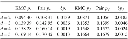
Next, consider thed dependence of the boundaries of the regime of 2PC. As noted above, there is a direct correspon-dence between peq(111· · ·)=pe (the upper boundary) in KMC analysis and MF-type treatments. However, due to APF, peq(100· · ·) in MF-type treatments does not correspond to the lower boundary pf of the 2PC regime (as it does in KMC analysis). We claim thatpfcan be estimated in MF-type treat-ments from the stationary point for near-vertical interfaces with rare hyperskew steps, i.e.,pf =limS→∞peq(1000· · ·H S) as such steps eliminate APF. Support for this claim comes from

CHI-JEN WANG, DA-JIANG LIU, AND J. W. EVANS PHYSICAL REVIEW E85, 041109 (2012)

TABLE IV. KMC and pair estimates ofpeandpfand small errors

δpe(f)=pe(f)(pair) − pe(f)(KMC).

KMCpe Pairpe δpe KMCpf Pairpf δpf

d=2 0.094 40 0.108 31 0.0139 0.0871 0.1056 0.0185

d=3 0.139 39 0.142 95 0.0036 0.1353 0.1399 0.0046

d=4 0.158 28 0.160 14 0.0019 0.1548 0.1572 0.0024

d=5 0.169 14 0.170 42 0.0013 0.1664 0.1679 0.0015

the results in Table IV. The behavior pe(f)∼0.211 3765+

ce(f)/d as d → ∞, as determined from KMC analysis, is

confirmed from the MF-type analysis where the 1/d scaling is seen as a natural consequence of the form of the spatial coupling. As an aside, this strategy allows comparison of KMC and MF dRDE results for other orientations [25].

VII. CONCLUSIONS

Our analysis indicates shrinking of the width peq(d)≈ 0.014/dof the regime of generic 2PC associated with the dis-continuous transition in our QCP version of Schloegl’s second model on a hypercubic lattice with increasing dimensiond. Appropriate application of MF-type dRDEs is shown to be effective in elucidating this behavior particularly the scaling withd. These features and the utility of the dRDE analysis are expected to be general for nonequilibrium reaction models displaying discontinuous transitions. One could extend this analysis to consider nucleation of the more stable phase from the less stable one just outside the 2PC region. The orientation dependence of interface propagation will be reflected in the shapes of evolving droplets [10,11], a feature which again can be elucidated by a MF-type dRDE analysis.

A significant feature of the MF-type dRDE treatment is the appearance of APF. APF is artificial in the sense that it does not occur in the stochastic lattice-gas model due to fluctuations at the interface. Propagation failure in dRDEs of interest is in its own right [26–28]. Papers often identify a critical value in spatial coupling below which there exists propagation failure, behavior which is amplified upon further reducing this coupling [28]. These observations are consistent with our results, e.g., amplified APF for increasingd.

ACKNOWLEDGMENTS

This work was supported by the U.S. Department of Energy (USDOE), Basic Energy Sciences, Division of Chemical Sciences, Geosciences, and Biosciences, through the Ames Laboratory Chemical Physics and PCTC projects. The Ames Laboratory is operated for the USDOE by Iowa State Univer-sity under Contract No. DE-AC02-07CH11358.

APPENDIX A: PAIR dRDES

The pair approximation is applied to Eqs. (1) and (3)

for spatially inhomogeneous states corresponding to planar interfaces between active and vacuum states. For planar interfaces with a hyperskew (1111· · ·) orientation so that Ci1,i2,...,id=Ci1+i2+···+id =Cm, we letεm=1 − Cmdenote the probability that a site on the hyperskew plane m=

i1+i2+ · · · +id is empty. The probability of a NN empty pair with one site in planemand the other in planem + 1 is denoted byφm₊1/2. Then, the corresponding dRDEs have the

form

d/dt εm=p(1−εm)−(2εm−φm₊1/2−φm₋1/2)2/(4εm), (A1a) d/dt φm₋1/2=p(εm+εm₋1−2φm₋1/2)−φm₋1/2

×[d(εm−φm+1/2)2+2(d−1)

×(εm−φm+1/2)(εm−φm−1/2)

+(d−2)(εm−φm₋1/2)2]/[4d(εm)2]

−φm−1/2[d(εm−1−φm−3/2)2

+2(d−1)(εm−1−φm−3/2)(εm−φm−1/2)

+(d−2)(εm−φm₋1/2)2]/[4d(εm₋1)2]. (A1b)

These pair dRDEs reduce to those of the MF dRDEs in the limit asd → ∞.

For a vertical (1000· · ·) interface where Ci1,i2,...,id=Ci1=Cm, we letεm=1 − Cm. The probability of a NN empty pair with one site in planemand the other in planem + 1 [i.e., sites (i1,i2, . . . ,id) and (i1+1,i2, . . . ,id)] is denoted by φm₊1/2. In addition, we must consider the

distinct probabilityψmof the NN empty pair with both sites in planem. The corresponding dRDEs have the form

d/dt εm =p[1−εm]−[εm−ψm][dεm

−(d−2)ψm−φm₊1/2−φm₋1/2]/[dεm], (A2a) d/dt φm−1/2 =p[εm+εm−1−2φm−1/2]−φm−1/2[εm−ψm]

×[(d−1)εm−(d−2)ψm−φm₊1/2]/[d(εm)2]

−φm−1/2[εm−1−ψm−1][(d−1)εm−1

−(d−2)ψm−1−φm−3/2]/[d(εm−1)2],

(A2b) d/dt ψm =2p[εm−ψm]−ψm[εm−ψm][2(d−1)2εm

−2(d−2)2ψm−(2d−3)(φm₊1/2

+φm−1/2)]/[d(d−1)(εm)2]. (A2c) Examination of the form of Eqs. (A2) reveals that the active state cannot displace the vacuum state, consistent with exact behavior in the stochastic model.

APPENDIX B: dRDE PERTURBATION ANALYSIS FOR

VERTICAL INTERFACES ASd→ ∞

For a stationary planar vertical interface between the vacuum state on the left for m=0,−1,−2,. . ., and a populated state on the right for m=1,2,. . ., the MF dRDE

(11)implies that

p−Cm(1−Cm)=d−1(1−Cm)(Cm₊1−2Cm+Cm₋1)

for m1, (B1)

where C₀=0. For large d, the RHS is small which forces p−Cm(1−Cm)≈0 orCm≈Cact. Thus, it is natural to write

Cm=Cact−δm for m 1 where δm1 from which one

SCHLOEGL’s SECOND MODEL FOR AUTOCATALYSIS ON. . . PHYSICAL REVIEW E85, 041109 (2012)

TABLE V. Behavior ofδmversusmand versusdfrom a MF dRDE analysis for vertical interfaces atp=peq.

d δ1 δ2 δ3 δ4 δ5 δ6 δ6

10 0.1687 2.02×10−2 _22.0×10−4 _2.39×10−4 _2.58×10−5 _{2.78 ×10}−6 _3.01×10−7 100 0.0504 2.25×10−3 _9.79×10−5 _4.26×10−6 _1.85×10−7

1000 0.0161 2.44×10−4 _3.69×10−6 _5.57×10−8 10 000 0.0077 3.56×10−5 _1.67×10−7

obtains

(2C_act−1)δ₁−d−1C_act(1−C_act)−(δ₁)2−d−1(2−3C_act) ×δ1−d−1(1−Cact)δ2−d−1δ1(δ2−2δ1)=0, (B2a)

(2C_act−1)δm−d−1(1−Cact)(δm+1−2δm+δm−1)−(δm)2

−d−1δm(δm+1−2δm+δm−1)=0 for m >1. (B2b)

First, we consider the general case of a stationary interface for fixedp < peq(d) where 2Cact−1=(1−4p)1/2=O(1).

It follows from Eq.(B2a)where the first two terms dominate that d1 ≈d−1Cact(1−Cact)(2Cact−1)−1=O(d−1). Then,

considering the first two dominant terms in Eq.(B2b)implies that dm≈d−1(1−Cact)(2Cact−1)−1dm−1, which, in turn,

yields

δm≈Cact(1−Cact)m(2Cact−1)−md−m for m1. (B3)

Second, in the special case of a stationary interface for p=peq(d), one might anticipate distinct scaling behavior in the situation wherepeq(d)→ 1₄ asd → ∞. Indeed, analysis of numerical data in TableIIindicates that 1₄−peq(d)≈A/d where A ≈ 0.25 so that 2Cact−1=(1−4p)1/2≈B/d1/2

whereB ≈1.0. This forces modified scaling from Eqs. (B2) above. Now, the first three terms in Eq.(B2a)dominate, and one concludes thatB1 andδ1≈E/d1/2whereE= 1₂[B±

(B2₋₁₎1/2_{]. Then, considering the first two dominant terms in}

Eq.(B2b)imply thatdm≈ 1₂d−1/2B−1dm−1form >1, which,

in turn, yields

δm≈(2B)−m+1Ed−m/2 for m1. (B4) Data from numerical analysis of the MF dRDEs support this analysis. See TableV.

[1] J. Marro and R. Dickman,Nonequilibrium Phase Transitions in Lattice Models(Cambridge University Press, Cambridge, UK, 1999).

[2] G. Odor,Rev. Mod. Phys.76, 663 (2004).

[3] J. Cardy, Scaling and Renormalization in Statistical Physics (Cambridge University Press, Cambridge, UK, 1996). [4] F. Schloegl,Z. Phys.253, 147 (1972).

[5] P. Grassberger,Z. Phys. B: Condens. Matter47, 365 (1982). [6] J. P. Boon, D. Dab, R. Kapral, and A. Lawniczak,Phys. Rep.

273, 55 (1996).

[7] S. Prakash and G. Nicolis,J. Stat. Phys.86, 1289 (1997). [8] R. Durrett,SIAM Rev.41, 677 (1999).

[9] D.-J. Liu, X. Guo, and J. W. Evans,Phys. Rev. Lett.98, 050601 (2007).

[10] X. Guo, J. W. Evans, and D.-J. Liu,Physica A387, 177 (2008). Sites in the last two loss terms in Eq. (B1) are mislabeled. One should replaceiwithi − 1.

[11] X. Guo, D.-J. Liu, and J. W. Evans,J. Chem. Phys.130, 074106 (2009).

[12] X. Guo, Y. de Decker, and J. W. Evans,Phys. Rev. E82, 021121 (2010).

[13] C.-J. Wang, X. Guo, D.-J. Liu, and J. W. Evans,J. Stat. Phys. 144, 1308 (2011).

[14] A. L. Toom, inMulticomponent Random Systems, edited by R. L. Dobrushin and Y. G. Sinai (Dekker, New York, 1980). [15] C. H. Bennett and G. Grinstein,Phys. Rev. Lett.55, 657 (1985). [16] R. S. MacKay,Nonlinearity21, T273 (2008).

[17] For systems with finite linear sizeL, an alternative criterion is to balance rates for transitions between states due to homogeneous fluctuations. See G. Nicolis and J. W. Turner, Ann. N.Y. Acad. Sci. 316, 251 (1979); J. Ross, K. L. C. Hunt, and M. O. Vlad, J. Phys. Chem. C 106, 10951 (2002). Only for

LLc(characteristic interface width) does this criterion match stationary interfaces.

[18] R. M. Ziff, E. Gulari, and Y. Barshad,Phys. Rev. Lett.56, 2553 (1986).

[19] P. Fischer and U. M. Titulaer,Surf. Sci.221, 409 (1989). [20] J. W. Evans and T. R. Ray,Phys. Rev. E50, 4302 (1994). [21] R. H. Goodman, D. S. Graff, L. M. Sander, P. Leroux-Hugon,

and E. Cl´ement,Phys. Rev. E52, 5904 (1995).

[22] Y. De Decker, G. A. Tsekouras, A. Provata, T. Erneux, and G. Nicolis,Phys. Rev. E69, 036203 (2004).

[23] R. M. Ziff and B. J. Brosilow, Phys. Rev. A 46, 4630 (1992).

[24] J. W. Evans,Rev. Mod. Phys.65, 1281 (1993).

[25] KMC estimates forpeq(110· · ·) of 0.1390, 0.1576, and 0.1682 compare with pair estimates of 0.1425, 0.1594, and 0.1694 ford=3–5, respectively. KMC estimates forpeq(1110· · ·) of 0.1581 and 0.1688 compare with pair estimates of 0.1599 and 0.1700 ford=4 and 5, respectively.

[26] J. P. Keener,SIAM J. Appl. Math.47, 556 (1987).

[27] S.-N. Chow, J. Mallet-Paret, and E. S. Van Vleck, Int. J. Bifurcation Chaos6, 1605 (1996).

[28] G. Fath,Physica D116, 176 (1998).