Integrating Planning and Scheduling : A Constraint based Approach

(1)

A Constraint-based Approach

Debdeep Banerjee

A thesis submitted for the degree of Doctor of Philosophy of The Australian National

University

(2)

(3)

Except where otherwise indicated, this thesis is my own original work.

Debdeep Banerjee

(4)

(5)

(6)

(7)

(8)

Abstract

Automated decision making is one of the important problems of Artificial Intelligence (AI).

Planning and scheduling are two sub-fields of AI that research automated decision making. The

main focus of planning is on general representations of actions, causal reasoning among actions and domain-independent solving strategies. Scheduling generally optimizes problems with

complex temporal and resource constraints that have simpler causal relations between actions.

However, there are problems that have both planning characteristics (causal constraints) and scheduling characteristics (temporal and resource constraints), and have strong interactions

between these constraints. An integrated approach is needed to solve this class of problems

efficiently.

The main contribution of this thesis is an integrated constraint-based planning and

schedul-ing approach that can model and solve problems that have both plannschedul-ing and schedulschedul-ing

char-acteristics. In our representation problems are described using a multi-valued state variable planning language with explicit representation of different types of resources, and a new

ac-tion model where each acac-tion is represented by a set of transiac-tions. This acac-tion-transiac-tion model makes the representation of actions with delayed effects, effects with different durations, and

the representation of complex temporal and resource constraints like time-windows, deadline

goals, sequence-dependent setup times, etc simpler.

Constraint-based techniques have been successfully applied to solve scheduling problems.

Therefore, to solve a combined planning/scheduling problem we compile it into a CSP. This

compilation is bounded by the number of action occurrences. The constraint model is based on the notion of “support” for each type of transition. The constraint model can be viewed

as a system of CSPs, one for each state variable and resource, that are synchronized by a

simple temporal network for action start times. Central to our constraint model is the explicit representation and maintenance of the precedence constraints between transitions on the same

state variable or resource.

We propose a branching scheme for solving the CSP based on establishing supports for

transitions, which imply precedence constraints. Furthermore, we propose new propagation

and inference techniques that infer precedence relations from temporal and mutex constraints, and infer tighter temporal bounds from the precedence constraints. The distinguishing feature

of these inference and propagation techniques is that they not only consider the transitions and

actions that are included in the plan but can also consider actions and transitions that are not yet included in or excluded from the plan.

(9)

We conclude the thesis with a modeling case study of a complex satellite problem domain

to demonstrate the effectiveness of our representation. This problem domain has action choices

that are tightly coupled with temporal and resource constraints. We show that most of the complexities of this problem can be expressed in our representation in a simple and intuitive

(10)

Introduction

Automated decision making is one of the important problems of Artificial Intelligence (AI).

In AI, planning and scheduling are two sub-fields that research automated decision making. Although the goal of these two fields is the same, generating plans to achieve goals, they do

focus on solving different parts of the problem. The focus of planning is more on generality and reasoning about causalities between activities in a domain-independent way, while scheduling

traditionally focuses on resolving time and resource constraints for a given set of activities

where most of the causal relations are known. However, there are practical problems that have both planning and scheduling characteristics, and the interactions between these characteristics

are very tight. To solve this class of problems efficiently we need to integrate planning and

scheduling techniques.

AI planning problems are usually formulated with: an initial state, a goal state, and a set of actions. The task of a planning algorithm is to select and order a subset of actions , which is

called aPlan, such that if we execute the selected actions according to their ordering starting from the initial state, we will reach the goal state. For example, consider a problem where we have to plan a journey to the airport from home. We can either catch a bus or a taxi to go to the

airport. This means that there are two possible plans to achieve our goal (to be at the airport).

1. Plan-1: walk-to-bus-stop→get-in-bus→get-out-at-airport

2. Plan-2: walk-to-taxi-stand→get-in-taxi→get-out-at-airport.

Even though both plans are valid plans, they may fail during execution because these plans

ignored the temporal and resource constraints. A plan where each action has a start time is called a scheduleand the process of assigning start times to the actions is calledscheduling. A schedule is executable if it satisfies all temporal and resource constraints. The following

temporal information is given for our journey planning problem: we have to be in the airport within one hour, it takes 10 and 5 minutes to walk to the bus stop and taxi stand respectively

from home. A bus takes 50 minutes to reach the airport and the next bus is due in 15 minutes

time. A taxi will take 35 minutes to reach the airport. From this temporal information we can deduce thatPlan-1is not valid any more, because we have to be in the airport with an hour but

(15)

Plan-1will take at least 65 minutes ( 15 minutes before the next bus + 50 minutes traveling time). Plan-2remains valid, because we can reach to the airport before one hour using a taxi. Moreover, if we assume that the taxi would only accept cash as fare and we don’t have any cash, then we need to the consider extra action of going to an ATM. In this case, validity of

Plan-2would depend how far an ATM is from home and from the taxi stand. If this detour (home to ATM to taxi stand) takes more than 15 minutes, thenPlan-2will become invalid.

Like in the example above, there are many real life problems (for example, consider the satellite problem described by Smith et al. in [47]) that have complex action choices

(plan-ning) and a set of time and resource constraints (scheduling), and the interaction between the

consequences of action choices and the temporal and resource constraints is very tight. To make good executable plans (or schedules) for this class of problems we need to consider the

causal constraints together with the temporal and resource constraints at the same time.

In this thesis we propose a integrated system for solving this class of planning problems

that have tightly coupled planning and scheduling characteristics. In the remaining sections we first give a background on existing integrated planning scheduling systems. Then we will

briefly outline the contributions of this thesis.

1.1 Integrating AI Planning and Scheduling

Problems that are in between planning and scheduling usually share some common

complexi-ties like time-windows, resource constraints, complex alternative choices of actions, sequence dependent setup times on resources between actions etc. Most of these complexities, except

the action choices, can be seen as standard scheduling constraints. In general in these problems

there is a subset of actions that only need to be performed at most once, while there are other actions that may have to be executed more than once. This characteristic of having a set of

actions where each action occurs at most once has similarity with scheduling problems with

alternative actions choices (multi-mode scheduling [7]). The action choices in multi-mode scheduling problems are generally due to availability of alternative resources and/or different

action costs. There is a basic difference between these action choices in scheduling problems

and the class of planning problems that we want to solve. In multi-mode scheduling the action choices are generally causally independent and limited to a small fixed set of actions, while

problems in this “in-between” class often involve cascading sets of choices of actions that can

interact with each other in a complex way and it is not computationally feasible to enumerate all valid choices beforehand [47]. This means that the interactions between action selection

and ordering, and temporal and resource constraints are very strong in these problems.

There are mainly two types of modeling languages in the literature to model problems

(16)

[image:16.595.122.521.88.321.2]

model-§1.1 Integrating AI Planning and Scheduling 3

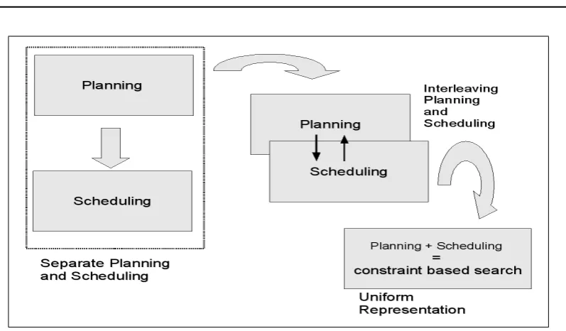
Figure 1.1: Planning scheduling integration

ing temporal and resource planning problems is PDDL2.1 [24]. PDDL2.1 can express most

of the complexities of our class of problems. Problems in PDDL2.1 are described using state

variables representing the state of the world, and actions with pre-conditions and effects whose execution changes one state to another. Timeline-based planning languages do not

explic-itly represent states or actions. Instead they keep track of evolution of each state variable

and resource (i.e. timeline) by placing tokens on timelines. Each token represents a change within a time interval. Individual tokens on state variable and resources are synchronized via

compatibility constraints (generally expressive temporal constraints). Another recently

pro-posed planning language ANML [15] tries to combine the best of both timeline-based and state/action-based modeling languages. We will discuss the similarities and the differences

between these languages and our representation in Chapter2.

There are different ways to integrate planning and scheduling techniques in a system. Smith et al. [47] classify the most common integration approaches into three types, as shown

in Figure1.1.

At one end of the spectrum, we can treat planning and scheduling as two different pro-cesses. First the planning process finds a plan that will achieve the goal, and then the scheduler

takes the initial plan and schedules the actions to satisfy the temporal and resource constraints.

One major problem of this approach is that not all valid plans are schedulable given a set of temporal and resource constraints. So when the scheduler fails to find a schedule, a new plan

has to be generated. This process will continue until a schedulable plan is generated. Although

(17)

The second possibility is to interleave planning and scheduling processes. This means that

whenever the planner chooses an action to achieve a goal condition, the scheduler posts

addi-tional ordering constraints between the selected action and other actions already in the plan, to satisfy temporal and resource constraints. The majority of the integrated planning and

schedul-ing systems are based on this idea. However, we can further distschedul-inguish these planners based

on their degree of interleaving. One example of loosely interleaved planning and scheduling technique is the temporal planner CRIKEY [29]. It uses a classical planner (FF [31]) together

with a simple temporal network (STN) [18] to generate a schedulable plan and then uses a

scheduler that generates a better quality temporal plan. Planners like Zeno [41], IxTeT [28], COLIN [13], Filuta [20], etc are more tightly integrated (i.e these systems do not use a separate

scheduling process to improve the quality of the plan) temporal planners based on the state-action representation. The emphasis of these planners is on generality of the representation

and finding domain-independent heuristics to solve planning problems efficiently. Examples

of planners that are based on timeline representations are HSTS [38], EUROPA [32], and OMPS [27]. Scalability is often a major problem for these systems. In most cases, it has been

necessary to use domain-specific search control for them to achieve acceptable performance.

However, recent work on domain-independent search control for timeline-based planners [6] may help overcome this problem in the future.

The third integration approach is to compile a problem with planning and scheduling

characteristics into a constraint-based search problem. Examples of this approach include

CPT [52], which takes a planning problem and converts it to a CSP [17], TM-LPSAT [45] which converts a problem to a combination of propositional logic and linear constraints, and

CTN [43], which converts a planning problem described in a timeline-based representation to

a CSP. The advantage of compiling a problem to constraint-based search is the availability of efficient solvers. In particular, converting to a CSP has the added advantage of being able to

ex-ploit the advancements in constraint-based scheduling [23] techniques. Note that planners that

interleave planning and scheduling processes also use constraint-based scheduling techniques for temporal and resource reasoning. The difference between the compilation and interleaving

approach is that in the latter approach planning and scheduling decisions are kept separate.

Constraint-based scheduling is popular because of its power of inference for deducing

tighter bounds on temporal variables. There are two main categories of inference techniques: one is based on absolute temporal information and the other is based on relative temporal

information. Examples of the first kind of inference techniques include Time-Tabling [4],

Not-First-Not-Last [50], Edge-Finding [40] etc. Examples of the second class of inference techniques include the Balance and the Energy Precedence constraints [36]. Inference

tech-niques based on relative temporal information are very important for solving problems with

(18)

§1.2 Overview of Contributions 5

temporal variables, but maintain the precedence order between activities.

1.2 Overview of Contributions

The main contribution of this thesis is an integrated constraint-based planning and scheduling

approach that can model and solve problems that have both planning and scheduling

charac-teristics. Our approach is to compile a planning problem described in our state/action-based representation to a CSP. To solve this CSP efficiently we have developed a new branching

strategy and several new propagation and inference techniques.

In our representation, problems are described using a multi-valued state variable planning

language (like in, for example, SAS+[2]) with explicit representation of different type of re-sources and a new action model. In our action model each action is represented by a set of

transitions, where each transition represents either an effect on a state variable or a resource

requirement of the action. This action-transition model makes the representation of delayed effects and effects with varying duration of actions simpler. Chapter2presents the basics of

our representation in detail. Complex temporal and resource constraints like time-windows,

deadline goals, sequence-dependent setup times etc, can be expressed in this representation in a simple and intuitive way. In Chapter5we describe how these features are added on top

of the basic representation. We demonstrate modeling of a complex satellite domain in our

representation in Chapter6.

A problem described in our representation is solved by compiling it into a CSP. This com-pilation is bounded by the number of action occurrences (similar to the planner CPT). The

constraint model is based on the notion of “support” for each type of transition, where the

meaning of “support” is similar to that of acausal link in partial-order planning (POP) [55]. In this thesis we extend the concept of causal links to resource transitions which are called

“support links”. The constraint model can be viewed as a system of CSPs, one for each state

variable and resource, that are synchronized by a simple temporal network (STN) for action start times. Central to our constraint model is the explicit representation and maintenace of the

precedence constraints between transitions on same domain object. Chapter 3 describes the

compilation process and the constraint model.

We propose a branching scheme based on establishing causal and support links, which imply precedence constraints. Furthermore, we propose several new propagation and inference

techniques that infer new precedence relations from temporal and mutex constraints, and infer

tighter temporal bounds from the precedence constraints. The main feature of these inference and propagation techniques is that they not only consider the transitions and actions that are

included in the plan but can also deduce new constraints for actions and transitions that are

(19)

for bounding temporal variables, and in addition they infer additional precedence constraints.

Chapter4describes our branching, propagation and inference techniques.

1.3 Publications

Part of this thesis is published in the following two conference papers, and a workshop paper:

1. Debdeep Banerjee. Integrating Planning and Scheduling in a CP Framework: A

Transition-Based Approach. In Alfonso Gerevini, Adele E. Howe, Amedeo Cesta, and Ioannis Refanidis, Editors, Proceedings of the 19th International Conference on

Automated Planning and Scheduling. AAAI Press, 2009.

2. Debdeep Banerjee and Patrik Haslum. Partial-Order Support-Link Scheduling. In

Fahiem Bacchus, Carmel Domshalk, Stefan Edelkamp, and Malte Helmert, Editors, Pro-ceedings of the21stInternational Conference on Automated Planning and Scheduling.

AAAI Press, 2011.

3. Debdeep Banerjee, Jason J. Li. Resource-based Planning With Timelines, In the

ICAPS Workshop on Planning and Scheduling with Timelines, PSTL 12, 2012.

The first paper describes the transition-based representation and compilation techniques for

temporal planning problems only involving state variables. The second paper describes the resource transitions and the CSP model for solving the single mode Resource Constrained

Project Scheduling Problems with min/max time lags (RCPSP/max). In this paper we

intro-duced the support link-based branching and inference techniques for resource transitions. We compared our method of creating partial order schedules for RCPSP/max problems with two

other approaches: a two stages approach that first finds a fixed point schedule and then lifts it to get a partial order schedule, and a envelope-based precedence constraint posting method.

The third paper describes a case study on how to model and solve a factory problem in our

(20)

Chapter 2

Modeling Planning and Scheduling

Problems

A systematic way of studying a problem is to model the problem of interest in some formal

specification and simulate different solving strategies by exploiting the specification. AI

plan-ning and scheduling problems are usually modeled using a set of interconnected components in a formal specification that describes the problem in terms of its components and

relation-ships between the components in a precise (mathematical) way such that an automated solving

mechanism (usually search) can be defined. A planning model usually reflects the reality of the problem domain. But to able to solve a problem, often we need to trade off between

expres-siveness of the model and the solution techniques’ efficiency. The more expressive a model is,

the harder it is to solve. So in general, a model is a sufficient approximation of the real world, such that we can solve these problems efficiently. Although modeling is an important part of

solving problems, in reality it’s quite hard and time consuming and sometimes impossible to

model a problem close to reality. It will always have to be an approximation. There is now research on how to solve problem with incomplete models [33].

The problems that we want to model and solve in this thesis are the problems that are in between planning and scheduling problems. In this type of problems, things that needed to

be modeled are the domain objects such as states of the components and resources, and how

these objects interact with each other via actions. For the planning part we need to model the causal interaction between actions, that describes how one action can enable another action,

and for the scheduling part we need to model the validity of these interactions by making

sure none of the domain objects are in an invalid state at any point in time. In this thesis we assume a deterministic model of actions under the closed-world assumption, meaning that

we know exactly the effects of each action and only actions change the state of components

of the planning problem. All the numeric quantities in our model, like durations, resource requirements, capacities of resources, time etc. are integer values.

(21)

2.1 Background and Related Work

There are many representation languages to represent planning problems. The most com-monly used representation languages in the planning community are PDDL [1] and its variants.

PDDL1.2, provides language constructs for classical planning problems based on STRIPS,

where actions have instantaneous effects. Successors of PDDL1.2 such as PDDL2.1 [24] ex-tends to temporal planning via introducing durative actions and continuous numeric variables,

and define semantics for concurrency and temporal constraints. Generally, AI planning mod-els are based on a description of the world in terms of propositional and numeric variables and

functions defined over them, and actions that have pre- and post-conditions that changes the

world. Although PDDL is used widely in the planning research community (due to the fact that there are lot of example problem domains available, as it is being used as the official language

for International Planning Competitions), its not easy to model practical problems mainly due

to its propositional nature and lack of support for modeling different kind of resources and different temporal constraints that occur in many real world problems. Scheduling [9] problem

models are generally described by available resources and durative activities that have different

requirements on these resources. Alternative options to achieve goals are generally represented by different modes of action execution. In general scheduling lacks a representation language

that can be used to model problems in a high level description.

Other attempts have been made to represent problems that are in between planning and scheduling. A concrete approach was introduced in HSTS[38], called HSTS-DDL. The main

idea was to represent planning and scheduling problem as a dynamic system model. This

method was inspired by approaches in control to synthesize valid behaviors of dynamic sys-tems. The main difference between this approach and PDDL-type planning representations is

that in this approach a planning problem is described as set of timelines instead of proposi-tional state variables, and there is no concept of a global state or actions. A timeline represents

the temporal evolution of some feature of a component of the problem domain over a planning

horizon. Each feature can have more than one state that it can assume, but can be only in one state at any time point. Each timeline is described by a set of temporal intervals, called tokens.

A token on a timeline describes the state of the feature, that the timeline represents, over the

interval. Since a feature can be only in one state at any time, this means tokens on a timeline are totally ordered and there is no time-gap between the end of a token and the start of the next

token. Tokens are constrained with other tokens (on the same timeline or on different timeline)

via compatibility constraints. To solve a problem, the task is to allocate and order tokens on each timeline, such that all compatibility constraints are satisfied, and at the end of the planning

horizon states of the timelines satisfy the goal. The timeline-based planning problem

(22)

§2.1 Background and Related Work 9

of the domain and the working of constraint-based solving strategies.

Recently, ANML [15] was introduced as a modeling language for planning and

schedul-ing problems that tries to take best of both PDDL and timeline based representations. This language represents planning problem with multi-valued state variables (as in timeline-based

languages) and has notions of actions and states (as in PDDL-based languages). It represents

resources as bounded numeric fluents (like PDDL-based languages) and supports expressive temporal constraints (as in timeline-based languages). ANML supports both generative and

HTN planning. Although it provides an expressive language to represent planning and

schedul-ing problems, there is yet no planner that solves a plannschedul-ing problem described in ANML. In this section we describe the representation that we will be using to model planning

problems. This representation is based on the multi-valued state variable representation of planning problems, with the following extensions:

• In our representation we explicitly represent resources as domain objects. Usually in

AI planning resources are represented as numeric fluents. In most real world problems,

resources can be easily identified and they have structure. That means, resources in real

world are more constrained w.r.t how they can be used than general numeric fluents. We would like to exploit this structure while reasoning about them by making different types

of resources explicit in the representation.

• We represent actions as a set of synchronized durative effects, where these effects can

have different durations. We call these durative effects of actions Transitions. This means that in our representation, instead of talking about the durations of actions, we talk

about the durations of transitions of actions. In planning and scheduling representations,

generally durations are associated with actions, which forces each effects of an action (or resource requirement of an activity in the scheduling case) to have same duration.

The motivation behind our action representation is to allow modeling of a actions where

effects can have different durations. For example, in a factory planning setting, lets say action MAKE-P 1-M 1 represents making of Product 1 in Machine 1 and it takes 15 units of time to make the product. This means thatMAKE-P 1-M 1 needsMachine 1, which is a resource, for 15 units of time. It also needs a worker to configureMachine 1, but only for the first 5 units of time. To model this action either in PDDL or in standard

scheduling model we need two actions (or activities), where the first one action requires

a worker andMachine 1for 5 units of time, and produces the precondition of the second one, and the second action needs Machine 1 and makes the product Product 1 in 10 units of time. In our presentation this can be achieved using only one action with two

different effects that start at the same time, but the first one requires the machine for 15 units of time, and the second one requires a worker for 5 units of time.

(23)

description, that expresses the time delay between start of the transition and start of its

action. This allows us to model delayed effect of actions.

• Each action effect (transition) is typed depending on if the transition is on a multi-valued

state variable or on a resource.

The main aim here is to make the modeling task as simple as possible for the domain modeler

and provide a flexible way to describe complex actions. Our representation is closely related

to the ANML language. Like ANML we also describe a planning problem with multi-valued state variables, and have notion of action. The differences are:

• Our representation only supports generative planning, where ANML can also support

HTN planning.

• Our representation explicitly represents resources as domain objects, where ANML

de-scribes resources as bounded numeric fluents.

• ANML provides temporal qualifiers that helps to represent expressive actions. In our

representation we introduce a different action model where each action is described by a set of transitions. It our action model, actions can have only certain types of transitions,

where each type has a clear semantics how they affect state variable and resources.

Al-though this restricts our representation to express arbitrary effects of actions, it helps us to develop a solution technique that is described in the next chapter.

The planning language used by the partial-order planner IxTeT [28] is also closely related

to our representation. In this representation, changes caused by actions are instantaneous. The problem with instantaneous change is that the domain modeler becomes responsible for

ensur-ing the safe execution of actions on state variables and resources. We represent changes as

tran-sitions which can encapsulate complex durative processes of change. Especially on a resource, it is complicated to represent such complex durative processes using instantaneous resource

events in a way that guarantees safe execution. This is also why ANML represents

consump-tions and producconsump-tions of resources as transiconsump-tions [15]. We believe that transitions make the domain modeler job easier to ensure the safe execution of actions (see Section2.2.3.4).

2.1.1 Base representation and extensions

In the following sections we describe our planning problem representation in detail. First we describe the components of our base representation, which includes resources, state variables

and actions. Then we describe the planning problem in terms of these components, initial

(24)

§2.2 Components of a Planning Model 11

that transforms the planning problem described in the base representation to a constraint

sat-isfaction problem. To keep the base representation, and its compilation to a constraint model,

simple, it does not include explicit representation of common scheduling constraints such as setup time, deadlines, time-windows etc. Instead, in Chapter5we will show how these

con-straints can be modelled as add-on concon-straints on top of the constraint model generated from

the base representation. In Chapter6we will demonstrate the modeling of a complex satellite problem using the extended representation.

2.2 Components of a Planning Model

To model a planning problem, we need to model the planning world and actions that manipulate

the world. By planning world we mean the collection of domain objects relevant to problem, that can be in different states. For example, for a factory planning problem, the planing world

can consist of machines, workers, products, orders etc. Actions are the components that

ma-nipulate the planning world by changing one or more domain objects states. For example, making a product is an example of an action for factory planning that changes the state of the

product from not-yet-made to made, and changes the state of a machine from available to not

available during execution.

The planning model in our representation consists of three components: Resources, State Variables1_{and Actions. Resources and state variables are the domain objects that describes the}

state of the world. Resources and state variables evolve over time, meaning that the availability

of resources and the state of state variables changes over time.

We view state variables and resources astimelinesas described in control-based modeling of planning and scheduling problems. That means by timelines of state variable and resource we will mean their evolution over time in terms of states and resource availability.

2.2.1 Resources

Resources play an important role in most realistic planning and scheduling problems. Any

ob-ject that enables an action to execute can be thought of as a resource. For example, in a factory planing problem machines, workers, raw materials to produce goods, and money are examples

of resources. In general resources can be categorized in different types [5,49] depending on if

a resource can be consumed, produced, usage is either discrete or continuous, if the capacity of a resource changes over time etc. For example, raw material in a factory scheduling problem

can be considered as a consumable resource as actions need to consume raw materials to

pro-duce goods, and in the process generate waste materials that can be considered as producible resource, which enables a cleaning action to execute. On the other hand, money can be seen

(25)

as a both producible and consumable resource as paying workers wages consumes money and

selling products to customers produces money for the factory.

Resources that appear in real world problems can be categorized in the following two broad categories, based on what the way they can be accessed:

• Reservoir Resource: This is a resource that can be either consumed by actions at the

beginning of execution or produced by actions at the end of execution. For example, consider an inventory that has finite capacity to store finished products in a factory. Each

produced good needs to be stored before it can go out to a customer, where it consumes some space in the inventory, and when it is delivered to the customer it produces the

same amount of space in the inventory.

• Reusable Resource: This is a resource that can be borrowed by actions at the beginning

of their execution, and returned with the same amount at the end of the execution. An example of this kind of resource is a machine in a factory. When an product is being

made in a machine, it borrows the machine until it finishes. No other products have

access to the machine during this time.

In this thesis we assume all resources have constant integer capacity. This means that the

capacity of resources does not change with time and can only be required by discrete integer

amounts.

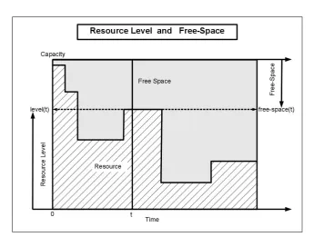
2.2.1.1 Resource Model

For each resourcer, capacity(r)represents the integer capacity of resource r, which repre-sents maximum amount of resource available at any point in time. Note that resources have

constant capacity over time. If capacity(r) = 1, we will call the resourceUnit-Capacity Resource, otherwise we will call r aMulti-Capacity Resource. Lettype(r)denote the type of the resourcer which can be either ReusableorReservoir. To reason about action execu-tion, it is important to track the amount of resource available at any given time point. For

any given time point t, let level(r,t) represent the amount of resource available to use at that time point. Note thatlevel(r,t)is an non-negative integer and bounded within the range

[0, capacity(r)]. When level(r,t) = 0 it means there is no resource available, and when

level(r,t) = capacity(r)it means resource is full. level(r,t)can be seen as the resource

profile function of r, as defined by Cesta et al [12]. Similarly, let free-space(r,t) denote how much free space is there in the resource at a given timet. The variablefree-space(r,t)

is the complement2 of the variable level(r,t). Note that, at any time point t the invariant

free-space(r,t) +level(r,t) = capacity(r) holds. Sincefree-space(r,t) represents the complement of thelevel(r,t),0 ≤ free-space(r,t) ≤ capacity(r)also holds. Figure2.1

(26)

[image:26.595.145.502.95.356.2]

Figure 2.1: Resource Model

describes usage of a capacitate resource over time.

2.2.2 State Variables

State variables are the domain objects in the planning world that can be in one of many (finite) possible states at any given time. An action can either change states of a state variable from

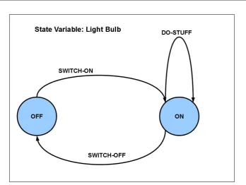
one to another, or require a particular state to hold during its execution. A simple example

would be a light bulb, that can be in two possible states: On and Off. Figure2.2 describes a transition graph of a state variable representing a light bulb. Nodes in the graph represent the

possible states. Edges are labeled with actions that either change states or require a particular

state. Action SWTICH-ON changes the state OFF to ON and similarly action SWITCH-OFF changes the state ON to OFF. Action DO-STUFF requires the state ON during its execution.

2.2.2.1 State Variable Model

For each state variablesv,dom(sv)represents the possible set of values (or states) thatsvcan assume. At any given time pointt, letstate(sv,t), denote the state ofsvatt.state(sv,t)can be seen as thetimelinefunction [43] of the state variablesv. At any time point t,sv can be either in one of its possible states or transiting from one state to another. The state of a state

(27)

[image:27.595.104.453.93.355.2]

Figure 2.2: State Variable: Bulb

v∈ dom(sv)∪ {∅}.

2.2.3 Actions and Transitions

Actions3are the components that manipulate the states of the domain objects. An action can change states of a subset of state variables from one state to another or requires a particular

state, and consume, produce or borrow resources. An action can have effects on one or more

state variables and resources simultaneously, and these effects can have different durations. This means that in our representation an action doesn’t have duration, its effects have durations.

Since we assign durations to the individual effects of actions, these effects become important

reasoning entities on their own right. We call each effect of an action aTransition.

Before we describe transitions of action, we want to make distinction between an action and an action instance. Anaction instanceis an occurrence of an action at a particular time. An

action can occur more than once in a plan. For example, consider an actionMove(truck,A,B), representing moving a truck from location A to location B in some logistics domain. Now if we say the actionMove(truck,A,B)starts at time pointt, then we mean that an instance of the action

Move(truck,A,B)starts att. There may be another instance of that action that starts at other time point. Note that multiple instances of an action can start at the same time. For example

consider an actionPRODUCE COALthat produces 10 units of coal from a coal mine. Now if

(28)

our goal is to produce 30 units of coal, then we can execute 3 instances ofPRODUCE COAL

action simultaneously. We always execute an action instance not an action. It means start time

is only defined for an action instance, not for an action. When we talk about the start time of an action, we mean the start time of an instance of that action. Note that multiple instances of

an action can have same start time. We consider each action instance as a unique entity.

We first describe transitions and how they affect evolution of the state variables and

re-source, then we describe the relationship between actions and its transitions.

2.2.3.1 Transition

A transitionT is always associated with an action instance. For each transitionT, letact(T)

denote the action instance this transition is part of,dur(T)denote the duration of transition T,req(T)represent the requirement of transitionT,start(T)andend(T)represent the start time and end time ofTrespectively. All transitions are non-preemptive, which means that they can’t be stopped after they start executing. This means that the following relation holds:

end(T) =start(T) +dur(T)

Depending on if a transition is executed on a resource or on a state variable, we define two main types of transitions: State Variable TransitionsandResource Transitions. In the

fol-lowing section we describe how state variable transitions and resource transitions are further

categorized depending on how they affect state variables and resources.

2.2.3.2 Transitions on State Variables

Each state variable transition can be either anEFFECT Transitionthat causes a state change, or aPREVAIL Transitionthat represents a persistent state requirement on the corresponding

state variable. In the following we describe these two types of transitions in details.

EFFECT Transitions: If a transition changes states of a state variable from one to another,

we will call this transition an EFFECT transition. On each state variablesv, the requirement of each EFFECT transition T_svE is a pair of states of the state variable, i.e. req(T_svE) =<

s_{f rom},sto >, where sf rom 6= sto and sf rom,sto ∈ dom(sv). It represents the fact that TsvE

achieves the statestofrom the statesf rom. The pre-condition of the EFFECT transitionTsvE is

the statesf rom, denoted aspre(TsvE) = sf rom, and the post-condition is the statesto, denoted

aspost(TE

sv) = sto. As described before for each state variablesv,state(sv,t)describes the

(29)

1. At the start of the execution the state ofsvmust be the pre-condition ofT_svE.

statesv, start(T_svE)=pre(T_svE) (2.1)

2. At the end of the execution the state of the state variablesvmust be the post-condition ofT_svE.

state(sv, end(T_svE)) =post(T_svE) (2.2)

3. During the execution at all intermediate time points between the start and the end ofT_svE the state of the state variable must be undefined i.e. ∅. It represents that an EFFECT

transition is executing onsv.

∀t s.t. start(T_svE)<t<end(T_svE): state(sv,t) =∅ (2.3)

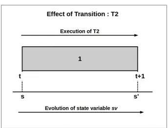
Figure2.3describes the effect of the execution of an EFFECT transitionT1on a state variable svthat hasdur(T1) = 6and achieves the states0fromswheres,s0 ∈dom(sv). Transition T1starts its execution at the time pointtand finishes at the time pointt+6. The state of the state variable issat time pointt, ands0at the time pointt+6, and all intermediate time points (fromt+1 tot+5) the state of the state variablesvisundefined. Note that if an EFFECT transitionT2, on the state variablesv, has unit duration (i.e.dur(T2) =1), and has the same requirement asT1, then there will be no intermediate time point where the state variablesv

would beundefinedas described in Figure2.4.

PREVAIL Transitions: If a transition does not change states of a state variable, but instead

requires a particular state for the duration of its execution, we will call this transition a PRE-VAIL transition. Each PREPRE-VAIL transition T_svP on a state variable sv has the requirement

req(TP

sv) =< s >, wheresis a possible domain value of the state variablesv, meaning that

the state variable must have the state s during the execution of T_svP. That means at all time points during the execution ofT_svP the the state ofsvmust bereq(T_svP).

∀t0 s.t. start(Tsv)≤t0 ≤end(Tsv): state(sv,t0) =req(TsvP) (2.4)

Example: Recall the example of the state variable BULB given before. Now, consider that

there are two actions: SWITCH-ON-1 and SWITCH-ON-2 that have one EFFECT transition

each that changes the state of the BULB from OFF to ON. When the state of the bulb is

(30)

[image:30.595.146.494.110.374.2]

[image:30.595.146.491.429.692.2]

Figure 2.3: EFFECT Transition execution

(31)

of SWITCH-ON-2 action was executed or both EFFECT transitions of SWITCH-ON-1 and

SWITCH-ON-2 are executed simultaneously. Since our planning model is deterministic, we

assume that on each state variable,only one EFFECT transition can change states of the state variable at any given time. That means, if the bulb changes its state from

OFF-to-ON, then either one of the EFFECT transitions of SWITCH-ON actions must be executed, not

both. This assumption forces all EFFECT transitions that change states of the state variable to be totally ordered. Given a transition pairTsv andTsv0 on the state variablesv, we say that

they are totally orderediff eitherT_sv0 finishes its execution onsvbeforeTsvstarts its execution

orT_sv0 starts afterTsvfinishes, i.e. eitherstart(T)≥end(T0)orstart(T0)≥ end(T)holds.

On the other hand, a PREVAIL transition requires a state variable to be in a particular state

during its execution. If there are other PREVAIL transitions that requires the same state, then they can be executed parallely. Since EFFECT transitions change state of state variables, each

PREVAIL transition on a state variable, must be totally ordered with all EFFECT transitions

on the state variable.

State Variable as Resource:Each state variable, where all transitions on a state variable have

to be totally ordered, except for the PREVAIL transitions on the same state, can be viewed as discrete-state resource, as described by Smith et al [49]. In a unit-capacity resource, only one

action can use the resource at time, meaning all actions that need the resource must be totally

ordered in the final solution. In case of a state variable, at most one EFFECT transition can change the state of state variable at any time. In the final plan, all EFFECT transitions that

change states of the same state variable must be totally ordered.

2.2.3.3 Transitions on Resources

For a resourcerand a given time pointt,level(r,t)represents the amount of resource available for use, and its dualfree-space(r,t)4represents the amount of free-space on the resource. The level of resources (also the amount of free-space) changes only via execution of transitions on

resources. We describe the effects of transitions at each time point during their execution intervals on resources via three resource events : production,consumption, and reservation. Production and consumption events have their usual meaning, that is production (increament

of level) and consumption (decreament of level) of resources. When we say”a transitionT reserves req(T) amount of free-space on the resourcer at the time point t”, we mean that at time pointt the amount of free-space onr must be greater than or equal toreq(T). That means:

reserve(req(T),t)⇒free-space(r,t)≥req(T)

(32)

[image:32.595.168.472.107.342.2]

Figure 2.5: PRODUCE Transition execution

Note that a reservation request for a transition T at the time point of t doesn’t change the

amount of free-space onr but posts the above condition that must hold ifTis executed onr. The reservation requests of transitions are additive. For example, if there exists two transitions TandT0such that at time pointtthey reservereq(T)andreq(T0)amount of free-space onr, thenfree-space(r,t)must be greater than or equal toreq(T) +req(T0).

In our representation, a resourcercan be either areservoirresource or areusableresource. On reservoir resources, transitions can either produce or consume resource, and on resuable

re-source transitions can only borrow rere-source during their execution intervals. First we describe how transitions consume and produce resources on reservoir resources, and then based on the

transitions defined on reservoir resources we describe how reusable resources are affected by the transitions on them.

On a reservoir resourcer, a transitionTrcan either produce or consumereq(Tr)amount

of resource during their execution. Note that production events increase the level of resource and consumes free-space, and similarly consume events decrease resource level and produces

free-space. On each reservoir resource we define two types of transitions as following.

PRODUCE transition: Each PRODUCE transitionTP

r that starts its execution atstart(TrP),

(33)

[image:33.595.123.432.103.342.2]

Figure 2.6: CONUSUME Transition execution

CONSUME transition: Each CONSUME transition T_rC consumesreq(T_rC)amount of re-source at the time pointstart(TC

r ), andreservesreq(TrC)amount of free-space at each time

point fromstart(T_rC)toend(T_rC)−1. Figure2.6describes the effect of execution of a CON-SUME transitionTthat has duration 3. Tconsumesreq(T)amount of resource at the starting time pointtandreservesreq(T)amount of free-space from the time pointtto the time point t+2.

Transitions on reusable resources can’t consume or produce resources separately as in

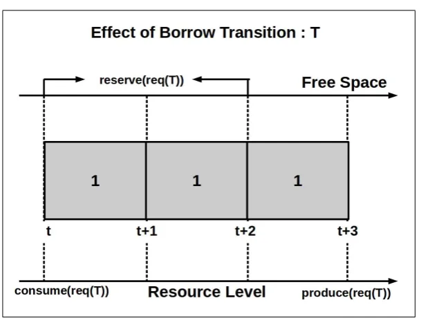
reservoir resource. Transitions on reusable resources can onlyborrowresources during their execution. We define the type for transitions on reusable resources as the following:

BORROW transition: Each transitionT_rBon a reusable resourceris called a BORROW

tran-sition that borrowsreq(TB

r)amount of resource at start and returns the same amount at the end.

Each BORROW transition with durationdcan be seen as a sequence of two (non-overlapping) consecutive transitions, where the first one is a CONSUME transition with durationd−1and

the second one is a PRODUCE transitions with unit duration. Each BORROW transition TB r

consumesreq(T_rB)amount of resource atstart(T_rB),reservesreq(T_rB)amount of free-space at each time point from start(T_rB) to end(T_rB)−1, and at end(T_rB) it produces req(T_rB)

amount of resource. Figure2.7 describes the effect of a BORROW transitionTthat has

(34)

[image:34.595.167.472.106.341.2]

Figure 2.7: BORROW Transition execution

2.2.3.4 Safe execution of transitions on resources

Although transitions have positive non-zero durations, we assume that consumption events occur at the start of the transition execution and production events occur at the end of the

transition execution and these events change the level of resource available. Note that at

any time point t the level of a resource r must be within the capacity of the resource, i.e.

∀t : 0 ≤ level(r,t) ≤ capacity(r). Each production event consumes free-space and each consumption events produces free-space on the resource. At any time pointt,free-space(r,t)

that represents the amount of free-space on the resource att, which is the dual oflevel(r,t). By allowing transitions toreservefree-space, we enable safe execution of the durative

transi-tions on resources.

Definition 1. Safe Execution

A safe execution of transitions on a resourcer, is a execution where at each time pointt, the invariant0≤level(r,t)≤capacity(r)holds and the total reservation request for free-space on the resource is less than or equal tofree-space(r,t).

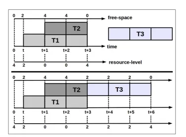
Consider a reusable resource with capacity 4 that has three BORROW transitions T1,T2,

andT3, where all of them require 2 units of resource,T1andT3have duration 3, andT2has duration 2. Figure2.8(top) describes an execution situation whereT1starts its execution att,

(35)

[image:35.595.90.468.94.372.2]

Figure 2.8: Safe execution on reusable resource

units of resource each. At each time point, total required free-space reservation is satisfied and at each time point sum of amount of free-space and resource level is 4 (capacity of the

resource). It means that execution ofT1andT2on the resource is a safe execution. Now if we

want to executeT3on the resource, we can see that ifT3starts at any time point betweentand t+2, then the execution would not be safe. Because ifT3starts at any time point betweent andt+2, then att+1andt+2the total reservation of free-space would be 6 (each transition would reserve 2 units of free-space), which would be greater than the available free-space on the resource. SoT3can not start at any time pointt0, wheret−2≤ t0 ≤ t+3. The bottom part of the Figure2.7describes one possible safe execution ofT1,T2andT3on the reusable resource, whereT3starts att+3.

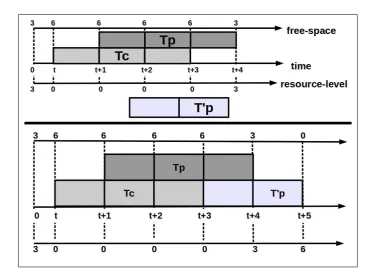
Figure2.9describes an example of transition execution on a reservoir resource. The

reser-voir resource has capacity 6, at start (time point 0) 3 units of resource is available for use, and a CONSUME transitionTcstarts its execution attand a PRODUCE transition starts att+1. At tthe level of resource reduced to 0 becauseTcconsumes 3 units of resource at start, and

att+4 T p produces 3 units of resource. At the top part of the Figure 2.9 describes a safe execution of Tcand T p on the resource. Given another PRODUCE transitionT0p that has

duration 2 and produces 3 units of resource, we can see that theT0pcan start earliest att+3

(36)

[image:36.595.130.510.99.371.2]

Figure 2.9: Safe execution on reservoir resource

when it produces resource. T0p can’t finish at t+1or t+2, because then it will consume 3 units of free-space at those time points, and the execution of Tcand T p will not be safe.

IfT0p finishes at time pointt or before, then amount of free-space in the resource will be 3.

Since there are no other CONSUME transition (that can produce free-space) to execute on the resource, execution ofTcandT pwould become unsafe att+1andt+2. Which means that T0pcan’t finish at any time point beforet+2(includingt+2) such that the executionTcand T premains safe. This means thatT0pcan’t start any time point beforet(sinceT0phas dura-tion 2). So we can conclude on the reservoir resource the execudura-tion of transidura-tions whereT0p

start earliest att+3and produce 3 units of resource att+6, is a safe execution as described in the bottom part of the Figure2.9.

2.2.3.5 Conservative Modeling of Resource Transitions

In general, each resource transition of actions consumes or produces at a different or fixed

rate during their execution. For example, consider two actions AC and AP that consumes

and produces resource r respectively, where r is a reservoir resource with capacity(r) =

10. Figure2.10 describes the consumption of AC and production of AP on the resource r.

Durations of both these effects are 4. ActionAC consumes resource at different consumption

(37)

Figure 2.10: Conservative Modeling of Action Resource Usage

its execution. Similarly, action AP produces total 8 units of resource at a fixed rate of 2 units

per unit of time during its execution.

In our representation we model consumption effect of AC as a CONSUME transitionTc

that consumes the total consumption amount at the start of its execution, i.e. req(Tc) = 9. Similarly we model the production effect of AP as a PRODUCE transitionT pthat produces

the total production amount at the end of its execution, i.e req(T p) = 8. Both transitions Tc and T p have duration 4. This way of approximating the effects of actions can be seen ascoarse-grained discretization, where we lose the information about the consumption or

production process at each time-step during the execution interval of transitions. Because

of this coarse-grained discretization, we have the conservativeassumption that each type of transition reserves free-space during its execution. This conservative assumption ensures that

execution of transitions on a resource will besafe.

One disadvantage of the conservative assumption is that it delays the start of transitions, where the transition could be executed earlier time in real world onreservoirresources. For ex-ample, consider the execution situation described in Figure2.11, where there are no other

tran-sitions except forTcandT pare executing onr, and at the beginningris full, i.e.level(r, 0) =

capacity(r) = 10. If we assume start(Tc) = t, then att, 9 units of resource is being con-sumed by Tc. It means at t there exists 1 unit of resource and 9 units of free-space on the

(38)

Figure 2.11: Coarse-Grained Discretization

If we look at the Figure2.10, we can see if Tcstarts executing att, then earliestT pcan start executing is at the time pointt+2without overflowing or under-flowing the resourcer. We will describe latter how can we achieve this under the same conservative assumption using

our flexible action model that allows modeling delayed effects and multiple effects on same state variable and resource as described below. This enables discretization of the consumption

and production effects of actions at a finer level.

2.2.3.6 Action-Transition Model

As stated earlier that actions have transitions on state variables and resources. Each action

has a set (possibly empty) of transitions on each state variable and resource. Recall that, each transition is associated with an action instance. Here when we say that that an actiona

has a transition T, we mean that each instance of the actiona have a transitionT. For each

action a, for each state variable svand for each resourcer, leteffect(sv,a)andeffect(r,a)

represent the set of transitions that actionahas onsvandrrespectively. For each actiona, let

trans(a) = Ta

state∪ Tresa represent the set of transitions of the action, whereTstatea represents

the set of transitions on state variables, andTa

res represents the set of transitions on resources.

T_statea =[

∀sv

effect(sv,a)

T_resa =[

∀r

effect(r,a)

Note that, ifT ∈trans(a), thenact(T) =a.

(39)

that describes the delay between start of the actionaand start of the transitionTa. Start time

of transitions are synchronized with the start time of their actions via these offset values. This

means that, for each transitionTa, where Ta ∈ trans(a), the start time ofTa is related with the start time ofaas the following:

start(T) =start(a) +offset(T) (2.5)

It means that after actionastarts, transitionTstarts afteroffset(T)units of time.

In the PDDL-based representation each action has its duration and all effects take place

either at start or at the end of the action. Our action model differs from PDDL-based action

representation in two main ways: here actions do not have durations, instead the transitions of actions have durations, and the start of each transition can be delayed from the start of the

actions, which enables us to model complex actions that appear in many real world problems in a straight-forward way. Consider the example of the turning of a spacecraft in order to

point at a target, described by Smith [46]. To turn a space craft from one direction to other,

the reaction control system (RCS), must fire the thrusters to provide angular velocity, then the spacecraft coasts until it points to the destination target, then the RCS thrusters are fired again

to stop the angular motion of the spacecraft. It means the firing of the thrusters happens in the

beginning and the end, and is controlled by the controller. Each time the thrusters are fired, propellants are consumed and it creates vibrations which may prevent some other operation on

the spacecraft.

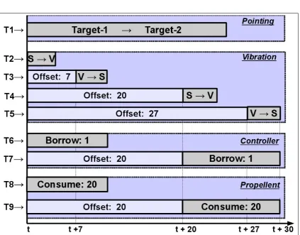
Assume that we have two state variables:Pointingthat represents the location of the point-ing device, whose domain consists of a finite set of targets, and Vibration representing the vibration status of the spacecraft which can take two possible values{V,S}, whereVstands

for “vibrating” andSstands for “stable”. There are two resources: a multi-capacity reservoir resourcePropellant, and an unit capacity reusable resource,Controller. In our representation we can model theTurnaction of the space craft fromTarget-1toTarget-2with the following sets of transitions. Each transition’s name is followed by its offset value and duration.

effect(Pointing,Turn) ={T1(0, 25)}

effect(Vibration,Turn) ={T2(0, 3),T3(7, 3),T4(20, 3),T5(27, 3)} effect(Controller,Turn) ={T6(0, 10),T7(20, 10)}

effect(Propellant,Turn) ={T8(0, 10),T9(20, 10)}

Figure2.12describes the pictorial view of the transitions of the Turn action. TransitionT1on

the state variablePointing changes the pointing location fromTarget-1toTarget-2and takes 25 units of time, and starts at the same time when the action starts. TransitionsT2 andT4on

(40)

[image:40.595.114.538.96.427.2]

Figure 2.12: Transitions of Turn Action

transitionsT3andT5change the the status from “vibrating” to “stable”. Each transition on the

state variableVibration takes 3 units of time, and have 0, 7, 20, and 27 as their offset values respectively. On the resourceController theTurn action has two borrow transitions T6 and T7, each borrows theControllerfor 10 units of time. T6 starts when the action starts, andT7

starts 20 units of time after the action starts. On the reservoir resourcePropellant, it has two consume transitions that consume 20 units of propellant while executing for 10 units of time.

Note thatT7onController andT9 onPropellantstarts after 20 units of time from the start of

the actionTurn.

In the PDDL2.1 durative action model, the assumption is that all the effects of an action,

must happen either at start of the action or at the end of the action. Due to this assumption, as Smith has argued [46], complex actions that have intermediate effects on state variables and

resources, like the Turn action described above, are not very easy to model with PDDL2.1. Our action model allows delays between the start of transitions and their corresponding actions that

provides a straight-forward way to model complex realistic actions.

(41)

except for PREVAIL transitions that require same state of the state variable. For each action we

can assume without loss of generality that all its PREVAIL transitions on a state variable are

non-overlapping, because if it has two PREVAIL transitions on different states, then those two PREVAIL transitions will be totally ordered, and if they are on the same state and overlapping

then we can always model them as a single PREVAIL transition.

This means, that for an action model to be valid, for each state variable, all transitions of

the action on the state variable must be sequenced, such that for each two transitionT1andT2,

whereT1appears beforeT2in the sequence, the following relation must hold.

offset(T2)≥offset(T1) +dur(T1) (2.6)

Similarly if an action has a set of overlapping resource transition on a resource, then total

requirement of the overlapping transitions must be less than or equals to the capacity of the resource. Note that, if for an action the above conditions do not hold, then we can trivially say

that the action will not be part of any solution.

2.3 Planning Problem Specification

A planning problem is defined asP =< Rreuse,Rreserve,SV,A,H,init,goal>, whereRreuse

andRreserveare the sets of reusable and reservoir resources respectively; SVis the set of state

variables; Ais the set of actions; H is the planning horizon;init is the initial configuration of the problem, andgoal is the goal description. Each resourcer ∈ Rreuse∪Rreserve has an

integer capacitycapacity(r). Each state variablesv ∈ SVhas a domain of statesdom(sv). Each action a ∈ Ahas a set of transitions (possibly empty) on each state variable and each resource, where each transitionTis a 5-tuple

T:< obj(T), type(T), dur(T), req(T), offset(T)>

whereobj(T)represents the state variable or resource that T requires, andtype(T)can as-sume one of the 5 types of transitions EFFECT, PREVAIL, BORROW, PRODUCE, and

CON-SUME. dur(T), req(T), and offset(T)have their usual meaning as defined before. Note that if a transition is a type of EFFECT, thenreq(T)is a pair of states, and if PREVAIL, then

req(T)is a state from the domain of obj(T), which is a state variable. If T is a resource transition, thenreq(T)is a positive integer.

We assume that our planning horizon starts from time 0 and ends at H. Note that the hori-zon is the time by which all goals of the problem must be achieved. In general, the horihori-zon can

be set to infinity.