Essays in Empirical Macroeconomics

(1)

E

SSAYS IN

E

MPIRICAL

M

ACROECONOMICS

W

EE

C

HIAN

K

OH

A THESIS SUBMITTED FOR THE DEGREE OF

DOCTOR OF PHILOSOPHY

OF THE

A

USTRALIAN

N

ATIONAL

U

NIVERSITY

(2)

ii

(3)

iii

Declaration

This thesis is my own work.

Chapter 2 is published in Oxford Economic Papers:

Koh, W. C. 2017. “Fiscal multipliers: new evidence from a large panel of countries.”

Oxford Economic Papers 69 (3): 569–90. doi:10.1093/oep

Chapter 3 is published in International Economics and Economic Policy: /gpw066

Koh, W. C. 2017. “Oil price shocks and macroeconomic adjustments in oil-exporting countries.” International Economics and Economic Policy 14 (2): 187–210. doi:10.1007/s10368-015-0333-z

Chapter 4 is published in Review of Development Economics:

Koh, W. C. 2017. “Fiscal policy in oil-exporting countries: the roles of oil funds and institutional quality.” Review of Development Economics 21 (3): 567–90. doi:10.1111/rode.12293

Chapter 5 is published in Journal of Southeast Asian Economies:

Koh, W. C. 2016. “Fiscal cyclicality in Brunei Darussalam.” Journal of Southeast Asian Economies 33 (1): 83–94. doi:10.1355/ae33-1e

Chapter 6 is published in The Singapore Economic Review:

Koh, W. C. 2016. “Sources of macroeconomic fluctuations in Brunei Darussalam.” The Singapore Economic Review. doi:10.1142/S0217590816500065

(4)

iv

Acknowledgements

First and foremost, I thank the Chair of my PhD supervisory panel, Warwick McKibbin. Warwick has been exceptional in providing guidance and advice. His sharp intellect and intuition grounded on economic principles and policy experience are clearly evident in our regular discussions and have influenced how I think about real-world issues. He has also been very encouraging and reassuring, which has given me confidence to pursue independent research. I would also like to thank my other panel members, Renée Fry-McKibbin and Joshua Chan, for their support and feedback on my work.

The stimulating intellectual environment at the Australian National University (ANU) has thoroughly enriched my PhD experience. I have forged enduring friendships and enjoyed the discussions with fellow PhD students from the Crawford School of Public Policy, Centre for Applied Macroeconomic Analysis (CAMA), Arndt-Corden Department of Economics, and Research School of Economics. In particular, I thank Dony Alex, Ben Ascione, Rohan Best, Alrick Campbell, Minhee Chae, Kimlong Chheng, Jamie Cross, Gan-Ochir Doojav, Ryan Edwards, Cody Hsiao, Shane Johnson, Anil Kavuri, Sanghyeok Lee, Anpeng Li, Larry Liu, Arjuna Mohottala, Matthew McKay, Bao Nguyen, Tomohito Okabe, Michinao Okachi, Manoj Pandey, Umbu Raya, Yashodha Pathirannehelage, Steve Thomas, Kai-Yun Tsai, Jiao Wang, Varang Wiriyawit, Benjamin Wong, and Jasmine Zheng.

I am appreciative of the comments received at the presentations I made at the CAMA Macroeconomics Brown Bag seminar, 11th Australasian Development Economics Workshop (ADEW), Singapore Economic Review Conference 2015, 28th

(5)

v

Anindya Banerjee, Fabrizio Carmignani, Rohan Fox, Timo Henckel, Stephen Howes, Asnawi Kamis, Phouphet Kyophilavong, Andy McKay, David Stern, Samuel Wills, Irene Yap, journal editors, and anonymous reviewers. I also acknowledge Jaromir Benes, Ryan Decker, and Inessa Love for sharing their MATLAB and Stata codes, which I adapted. Megan Poore has been extremely helpful in proofreading my papers.

I am honoured to represent Brunei Darussalam to participate in the 2016 U.S. Professional Fellows Program, sponsored by the U.S. Department of State, to understand how academic and policy research influence U.S. policymaking. I am grateful for the opportunity to meet with Congressmen and staff from the U.S. House of Representatives and the Senate, think tank professionals, and academic researchers. In particular, I thank Sarah Maxim for hosting my fellowship at the University of California at Berkeley. I also thank Donald Emmerson from Stanford University, Sunny Wong from the University of San Francisco, and James McGann from the University of Pennsylvania for accommodating my visits.

I am also fortunate to have secured full scholarship from the Centre for Strategic and Policy Studies, with funding provided by the Government of Brunei Darussalam. I thank Dato Paduka Haji Ismail Bin Haji Duraman and Diana Cheong for their approval and encouragement to pursue a PhD.

My parents and sister have always been supportive of my pursuits. I thank them for constantly believing in me.

(6)

vi

(7)

vii

Abstract

This thesis is a collection of five essays in empirical macroeconomics. The first paper evaluates the effectiveness of fiscal policy in different economic environments. The results show that, contrary to conventional wisdom, fiscal multipliers are not necessarily smaller in countries relatively open to trade and financial flows and operating under flexible exchange rates. The relationship between the size of fiscal multipliers and the three dimensions of openness—trade openness, capital mobility, and exchange rate flexibility—hinges on the response of the real exchange rate and the degree of monetary policy accommodation, which underscores the importance of fiscal and monetary policy interaction in understanding the fiscal transmission mechanism.

The second paper examines the effects of an adverse oil price shock in oil-exporting countries under alternative exchange rate and fiscal policy arrangements. The results show that output and government consumption fall, as expected, but the responses are smaller and smoother in countries with flexible exchange rates and oil funds. This highlights the shock-absorbing property of flexible exchange rates and the macroeconomic stabilization role of oil funds, making a case for oil exporters to adopt more flexible exchange rates and establish oil funds as fiscal buffers.

(8)

viii

The fourth paper examines the conduct of fiscal policy in Brunei, focusing on the cyclical patterns in government expenditure. In spite of relatively large fiscal buffers in Brunei’s oil funds, the results provide evidence of procyclical fiscal policy, which exacerbates the business cycle. This behaviour is primarily driven by procyclical current expenditure while capital expenditure is largely acyclical. A key policy recommendation would be to adopt clear fiscal rules to integrate the oil funds into the country’s macroeconomic policy framework to delink government spending from volatile oil revenue.

(9)

ix

List of Tables

2.1 Sign restrictions to identify a shock to fiscal spending ... 23

2.2 Im-Pesaran-Shin (IPS) panel unit root test ... 25

2.A1 Summary of selected panel data studies on the size of fiscal multipliers ... 51

2.A2 List of countries and structural characteristics ... 54

2.A3 Variables and data sources ... 61

2.B1 Kolmogorov-Smirnov equality-of-distributions tests of long-run cumulative fiscal multipliers in advanced and developing countries (Ilzetzki et al.’s (2013) country sample) ... 63

2.B2 Kolmogorov-Smirnov equality-of-distributions tests of long-run cumulative fiscal multipliers in countries with low and high trade openness (Ilzetzki et al.’s (2013) country sample) ... 64

2.B3 Kolmogorov-Smirnov equality-of-distributions tests of long-run cumulative fiscal multipliers in episodes of de facto fixed and flexible exchange rate regimes (Ilzetzki et al.’s (2013) country sample) ... 65

2.B4 Kolmogorov-Smirnov equality-of-distributions tests of long-run cumulative fiscal multipliers in episodes of low and high public debt (Ilzetzki et al.’s (2013) country sample) ... 66

2.C1 Kolmogorov-Smirnov equality-of-distributions tests of long-run cumulative fiscal multipliers in advanced and developing countries (120 country sample) ... 67

2.C2 Kolmogorov-Smirnov equality-of-distributions tests of long-run cumulative fiscal multipliers in countries with low and high trade openness (120 country sample) ... 68

(14)

xiv

2.C4 Kolmogorov-Smirnov equality-of-distributions tests of long-run cumulative fiscal multipliers in episodes of de facto fixed and flexible

exchange rate regimes (120 country sample) ... 70

2.C5 Kolmogorov-Smirnov equality-of-distributions tests of long-run cumulative fiscal multipliers in episodes of low and high public debt (120 country sample) ... 71

2.C6 Kolmogorov-Smirnov equality-of-distributions tests of long-run cumulative fiscal multipliers in episodes of low and high credit (120 country sample) ... 72

2.C7 Kolmogorov-Smirnov equality-of-distributions tests of long-run cumulative fiscal multipliers in episodes without and with financial crisis (120 country sample) ... 73

2.C8 Kolmogorov-Smirnov equality-of-distributions tests of long-run cumulative fiscal multipliers in expansionary and recessionary phases of the business cycle (120 country sample) ... 74

3.1 Oil-exporting countries and oil funds ... 108

3.3 Westerlund panel cointegration tests ... 110

3.4 Coefficients of oil price changes (negative) under fixed and flexible exchange rate regimes in various classifications ... 115

3.5 Coefficients of asymmetric oil price changes under fixed and flexible exchange rate regimes ... 120

3.6 Coefficients of oil price changes (negative) under different exchange rate and fiscal policy arrangements ... 123

3.A1 List of oil-exporting countries ... 127

3.B1 Coefficients of oil price changes (negative) under different exchange rate and fiscal policy arrangements; data period 1990–2010 ... 130

3.B2 Coefficients of oil price changes (negative) under different exchange rate and fiscal policy arrangements; advanced economies excluded ... 130

(15)

xv

3.B4 Coefficients of oil price changes (negative) under different exchange rate

and fiscal policy arrangements; control for institutional quality ... 131

3.B5 Coefficients of oil price changes (negative) under different exchange rate and fiscal policy arrangements; including money supply ... 132

4.2 Westerlund panel cointegration tests ... 141

4.3 Oil-exporting countries and oil funds ... 144

4.4 Oil-exporting countries and institutional quality score ... 145

4.5a Standard deviation of the growth rates of variables in high IQ countries ... 148

4.5b Standard deviation of the growth rates of variables in low IQ countries ... 149

4.6 Impulse volatility (over 8 periods) in response to a 10% oil price shock ... 153

4.7 Hypothesis testing of the difference in the response of government consumption to a GDP shock ... 156

4.A1 List of oil-exporting countries ... 162

4.C1a Hypothesis testing of the difference in the response of government consumption to a GDP shock with global demand and U.S. interest rate included in the model ... 167

4.C1b Impulse volatility (over 8 periods) in response to a 10% oil price shock with global demand and U.S. interest rate included in the model ... 167

4.C2a Hypothesis testing of the difference in the response of government consumption to a GDP shock with the order of GDP and government consumption reversed ... 168

4.C2b Impulse volatility (over 8 periods) in response to a 10% oil price shock with the order of GDP and government consumption reversed ... 168

4.C3a Hypothesis testing of the difference in the response of government consumption to a GDP shock with two lags in the model ... 169

4.C3b Impulse volatility (over 8 periods) in response to a 10% oil price shock with two lags in the model ... 169

4.C4a Hypothesis testing of the difference in the response of government consumption to a GDP shock with advanced economies excluded ... 170

(16)

xvi

4.C5a Hypothesis testing of the difference in the response of government consumption to a GDP shock with the sample period restricted to 1990–

2014 ... 171

4.C5b Impulse volatility (over 8 periods) in response to a 10% oil price shock with the sample period restricted to 1990–2014 ... 171

4.C6a Hypothesis testing of the difference in the response of government consumption to a GDP shock with hyperinflation periods removed ... 172

4.C6b Impulse volatility (over 8 periods) in response to a 10% oil price shock with hyperinflation periods removed ... 172

4.C7a Hypothesis testing of the difference in the response of government consumption to a GDP shock with the first three years of the oil fund period excluded ... 173

4.C7b Impulse volatility (over 8 periods) in response to a 10% oil price shock with the first three years of the oil fund period excluded ... 173

4.C8a Hypothesis testing of the difference in the response of government consumption to a GDP shock with national oil price series ... 174

4.C8b Impulse volatility (over 8 periods) in response to a 10% oil price shock with national oil price series ... 174

4.C9a Hypothesis testing of the difference in the response of government consumption to a GDP shock under large oil price changes ... 175

4.C9b Impulse volatility (over 8 periods) in response to a 10% oil price shock under large oil price changes ... 175

5.1 Estimation results using OLS and 2SLS ... 184

5.2 Unit root tests ... 185

6.1 Zivot-Andrews unit root test with a single structural break ... 204

6.2 Augmented Dickey-Fuller unit root tests ... 204

6.3 Johansen’s cointegration tests ... 205

6.4 Variance decomposition of domestic variables (%) ... 210

(17)

xvii

List of Figures

1.1 Average policy interest rates ... 3

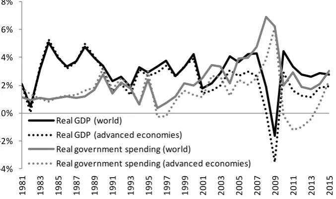
1.2 Average growth rates of real GDP and real government expenditure ... 3

1.3 Real crude oil price and number of new oil funds established ... 5

1.4 Crude oil price and Brunei’s GDP and government revenue ... 6

2.1 Cumulative fiscal multipliers in advanced and developing countries (Ilzetzki et al.’s (2013) country sample) ... 29

2.2 Cumulative fiscal multipliers in countries with low and high trade openness (Ilzetzki et al.’s (2013) country sample) ... 30

2.3 Cumulative fiscal multipliers in episodes of de facto fixed and flexible exchange rate regimes (Ilzetzki et al.’s (2013) country sample) ... 31

2.4 Cumulative fiscal multipliers in episodes of low and high public debt (Ilzetzki et al.’s (2013) country sample) ... 32

2.5 Cumulative fiscal multipliers in advanced and developing countries (120 country sample) ... 40

2.6 Cumulative fiscal multipliers in countries with low and high trade openness (120 country sample) ... 41

2.7 Impulse responses to a 1% government consumption shock in countries with low and high trade openness (120 country sample) ... 42

2.8 Cumulative fiscal multipliers in countries with low and high international capital mobility (120 country sample) ... 43

2.9 Impulse responses to a 1% government consumption shock in countries with low and high international capital mobility (120 country sample) ... 44

2.10 Cumulative fiscal multipliers in episodes of de facto fixed and flexible exchange rate regimes (120 country sample) ... 45

2.11 Impulse responses to a 1% government consumption shock in episodes of de facto fixed and flexible exchange rate regimes (120 country sample) ... 46

(18)

xviii

2.13 Cumulative fiscal multipliers in episodes of low and high credit (120 country sample) ... 48 2.14 Cumulative fiscal multipliers in episodes without and with financial crisis

(120 country sample) ... 49 2.15 Cumulative fiscal multipliers in expansionary and recessionary phases of

the business cycle (120 country sample) ... 50 2.B1 Empirical distributions of long-run cumulative fiscal multipliers in

advanced and developing countries (Ilzetzki et al.’s (2013) country sample) ... 63 2.B2 Empirical distributions of long-run cumulative fiscal multipliers in

countries with low and high trade openness (Ilzetzki et al.’s (2013) country sample) ... 64 2.B3 Empirical distributions of long-run cumulative fiscal multipliers in

episodes of de facto fixed and flexible exchange rate regimes (Ilzetzki et al.’s (2013) country sample) ... 65 2.B4 Empirical distributions of long-run cumulative fiscal multipliers in

episodes of low and high public debt (Ilzetzki et al.’s (2013) country sample) ... 66 2.C1 Empirical distributions of long-run cumulative fiscal multipliers in

advanced and developing countries (120 country sample) ... 67 2.C2 Empirical distributions of long-run cumulative fiscal multipliers in

countries with low and high trade openness (120 country sample) ... 68 2.C3 Empirical distributions of long-run cumulative fiscal multipliers in

countries with low and high international capital mobility (120 country sample) ... 69 2.C4 Empirical distributions of long-run cumulative fiscal multipliers in

episodes of de facto fixed and flexible exchange rate regimes (120 country sample) ... 70 2.C5 Empirical distributions of long-run cumulative fiscal multipliers in

episodes of low and high public debt (120 country sample) ... 71 2.C6 Empirical distributions of long-run cumulative fiscal multipliers in

(19)

xix

2.C7 Empirical distributions of long-run cumulative fiscal multipliers in episodes without and with financial crisis (120 country sample) ... 73 2.C8 Empirical distributions of long-run cumulative fiscal multipliers in

expansionary and recessionary phases of the business cycle (120 country sample) ... 74 2.D1 Cumulative fiscal multipliers in advanced and developing countries (120

country sample); standard SVAR ... 75 2.D2 Cumulative fiscal multipliers in countries with low and high trade

openness (120 country sample); standard SVAR ... 76 2.D3 Cumulative fiscal multipliers in countries with low and high international

capital mobility (120 country sample); standard SVAR ... 77 2.D4 Cumulative fiscal multipliers in episodes of de facto fixed and flexible

exchange rate regimes (120 country sample); standard SVAR ... 78 2.D5 Cumulative fiscal multipliers in episodes of low and high public debt (120

country sample); standard SVAR ... 79 2.D6 Cumulative fiscal multipliers in episodes of low and high credit (120

country sample); standard SVAR ... 80 2.D7 Cumulative fiscal multipliers in episodes without and with financial crisis

(120 country sample); standard SVAR ... 81 2.D8 Cumulative fiscal multipliers in expansionary and recessionary phases of

the business cycle (120 country sample); standard SVAR ... 82 2.E1 Cumulative fiscal multipliers in advanced and developing countries (82

country sample); standard SVAR ... 83 2.E2 Cumulative fiscal multipliers in countries with low and high trade

openness (82 country sample); standard SVAR ... 84 2.E3 Cumulative fiscal multipliers in countries with low and high international

capital mobility (82 country sample); standard SVAR ... 85 2.E4 Cumulative fiscal multipliers in episodes of de facto fixed and flexible

exchange rate regimes (82 country sample); standard SVAR ... 86 2.E5 Cumulative fiscal multipliers in episodes of low and high public debt (82

country sample); standard SVAR ... 87 2.E6 Cumulative fiscal multipliers in episodes of low and high credit (82

(20)

xx

2.E7 Cumulative fiscal multipliers in episodes without and with financial crisis (82 country sample); standard SVAR ... 89 2.D8 Cumulative fiscal multipliers in expansionary and recessionary phases of

the business cycle (82 country sample); standard SVAR ... 90 2.F1 Cumulative fiscal multipliers in advanced and developing countries (82

country sample); sign restrictions ... 91 2.F2 Cumulative fiscal multipliers in countries with low and high trade

openness (82 country sample); sign restrictions ... 92 2.F3 Cumulative fiscal multipliers in countries with low and high international

capital mobility (82 country sample); sign restrictions ... 93 2.F4 Cumulative fiscal multipliers in episodes of de facto fixed and flexible

exchange rate regimes (82 country sample); sign restrictions ... 94 2.F5 Cumulative fiscal multipliers in episodes of low and high public debt (82

country sample); sign restrictions ... 95 2.F6 Cumulative fiscal multipliers in episodes of low and high credit (82

country sample); sign restrictions ... 96 2.F7 Cumulative fiscal multipliers in episodes without and with financial crisis

(82 country sample); sign restrictions ... 97 2.F8 Cumulative fiscal multipliers in expansionary and recessionary phases of

the business cycle (82 country sample); sign restrictions ... 98 2.G1 Cumulative fiscal multipliers in advanced and developing countries

(Ilzetzki et al.’s (2013) country sample); standard SVAR ... 99 2.G2 Cumulative fiscal multipliers in countries with low and high trade

openness (Ilzetzki et al.’s (2013) country sample); standard SVAR ... 100 2.G3 Cumulative fiscal multipliers in episodes of de facto fixed and flexible

exchange rate regimes (Ilzetzki et al.’s (2013) country sample); standard SVAR ... 101 2.G4 Cumulative fiscal multipliers in episodes of low and high public debt

(Ilzetzki et al.’s (2013) country sample); standard SVAR ... 102 3.1 Exchange rate regime classifications of oil-exporting countries from 1973

to 2010 based on Ilzetzki et al. (2010) ... 108 3.2 Impulse responses to a -10% oil price shock under fixed and flexible

(21)

xxi

3.3 Impulse responses to a -10% oil price shock under alternative exchange

rate regime classifications ... 117

3.4 Impulse responses to asymmetric oil price shocks of 10% under fixed and flexible exchange rate regimes ... 119

3.5 Impulse responses to a -10% oil price shock under different exchange rate and fiscal policy arrangements ... 122

4.1 Stylized transmission of oil windfalls ... 139

4.2a Correlation of the cyclical components of GDP and government consumption in high IQ countries ... 146

4.2b Correlation of the cyclical components of GDP and government consumption in low IQ countries ... 147

4.3 Impulse responses of macroeconomic variables to a 10% oil price shock .... 152

4.4 Impulse responses of government consumption to a 1% GDP shock ... 155

4.B1 Impulse responses of the cyclical component of government consumption to a 1% GDP shock in the cyclical component of GDP ... 165

4.B2 Impulse responses of government consumption to an increase in institutional quality score of 0.1 ... 165

4.B3 Impulse responses of government consumption to a 1% GDP shock ... 166

4.B4 Impulse responses of gross capital formation to a 1% GDP shock ... 166

5.1 Cyclical component of real government expenditure and GDP ... 180

5.2 Percentage changes of real government expenditure and GDP ... 181

5.3 Cumulative impulse responses to structural shocks ... 187

5.4 Cumulative impulse responses to structural shocks, with real government current expenditure ... 188

5.5 Cumulative impulse responses to structural shocks, with real government capital expenditure ... 189

6.1 Data series plots of the variables in levels and first differences ... 203

(22)

1

Chapter 1 Introduction

1.1 Global economic events in the 21st century

The revival and intensification of global integration towards an open international trading and financial system has been at the core of multilateral economic policies since the Second World War. Although globalization can contribute to economic growth and improvements in development outcomes, at least in theory, this interdependence in the global village also inherently poses serious threats. The Dot-com bubble burst was the first significant economic event in the new millennium, which prompted policy responses to avert a deep recession. The Federal Reserve in the United States (U.S.) subsequently eased monetary policy, perhaps for too long. The loose monetary policy stance is argued to have a hand in sparking the refinancing boom in the U.S. (see Taylor, 2007), which led to the subprime mortgage crisis, collapse of the financial sector, and a real economic meltdown. This turmoil culminated in the Great Recession, drawing many parallels to the Great Depression in the 1930s (Temin, 2010; Eichengreen, 2015). The ensuing banking and financial crises in Iceland and Ireland, the sovereign debt crises in Portugal, Ireland, Italy, Greece, and Spain (PIIGS), and the chaos of Brexit and the European Union are testaments to the interconnectedness of the world economy.

(23)

2

and Blanchard, 2014; Husain et al., 2015; Vrontisi et al., 2015). However, the widely anticipated benefits have yet to materialize as the transmission channels to the real economy have become more complicated (Obstfeld et al., 2016). Global economic growth prospects remain bleak—the IMF and the Organisation for Economic Co-operation and Development (OECD) have repeatedly revised forecasts downwards (see IMF, 2016a; OECD, 2016).

1.2 Global fiscal stimulus

Monetary policy acted as the first line of defence in response to the GFC, but the limits of conventional monetary policy became increasingly apparent as policy interest rates in advanced economies approached the nominal zero lower bound (see Fig. 1.1). Fiscal policy was thus essential to aid in economic recovery. Many countries embarked on an unprecedented level of fiscal expansion unseen since the Second World War (Mauro et al., 2015), in the form of stimulus packages. The size of the fiscal stimulus in the G-20 countries was estimated at US$2 trillion, about 1.4% of 2008 world GDP (IILS, 2011). Figure 1.2 shows the large output fall and the sharp increase in real government spending during the GFC, but the stimulus was unwound in the following years as substantial fiscal deficits emerged. Against the current backdrop of a lacklustre global economy, the IMF and OECD are again advocating a coordinated fiscal stimulus response by the G-20 countries (IMF, 2016b; OECD, 2016).1

The effectiveness of fiscal stimulus has been an intensely political subject over the past several years. There is also little consensus among economists, owing to contradictory theoretical predictions and mixed empirical evidence. Identifying exogenous fiscal spending shocks is an important element in measuring the size of fiscal multipliers. The standard approach of Blanchard and Perotti (2002), by assuming government spending does not respond to GDP in the same quarter, requires quarterly data for the identification scheme to be valid. Data availability is a major obstacle to obtain reliable estimates, especially in developing countries, which typically only have annual time series data that are sufficiently long.

1

McKibbin and Stoeckel (2012) examine the consequences of global fiscal adjustments and highlight the

(24)

[image:24.595.122.460.97.302.2]

3 Fig. 1.1 Average policy interest rates

Notes: Data sourced from IMF International Financial Statistics. The averages are weighted by GDP in

current U.S. dollars.

Fig. 1.2 Average growth rates of real GDP and real government expenditure

Notes: Data sourced from IMF World Economic Outlook, April 2016. The averages are weighted by GDP

in current U.S. dollars.

An influential paper by Ilzetzki et al. (2013), based on a novel quarterly data set of 44 countries, finds that fiscal multipliers are smaller in developing countries, in countries relatively open to trade, under flexible exchange rate regimes, and when public debt is high. Interestingly, the estimated multipliers are negative in the long run. A sobering policy implication arising from the study is that fiscal stimulus could

0% 2% 4% 6% 8% 10% 12% 14% 16% 18% 20% 19 81 19 83 19 85 19 87 19 89 19 91 19 93 19 95 19 97 19 99 20 01 20 03 20 05 20 07 20 09 20 11 20 13 20 15

Interest rate (world) Interest rate (advanced economies)

-4% -2% 0% 2% 4% 6% 8% 19 81 19 83 19 85 19 87 19 89 19 91 19 93 19 95 19 97 19 99 20 01 20 03 20 05 20 07 20 09 20 11 20 13 20 15

Real GDP (world)

Real GDP (advanced economies) Real government spending (world)

[image:24.595.124.463.397.597.2]

(25)

4

become counterproductive due to increasing global integration and adoption of flexible exchange rate arrangements. However, Dellas et al. (2005) allude to the importance of fiscal and monetary policy interactions in determining the relationship between the size of fiscal multipliers and the degree of openness (trade openness, capital mobility, exchange rate flexibility). A corollary to this point is that there might, in fact, not be a systematic relationship.

1.3 The ‘new normal’ of low oil prices

Apart from the oil price crashes of 1985–86 and 1990–91, during which the Organization of the Petroleum Exporting Countries (OPEC) abandoned price targets and the First Gulf War respectively, crude oil prices remained relatively stable, hovering around US$30 per barrel in real terms between the mid 1980s and the end of the 20th century (see Fig. 1.3). The new millennium ushered in an era of oil price booms, reaching an apex of over US$140 per barrel in mid 2008. Oil prices fell dramatically during the GFC, but rebounded to over US$100 per barrel relatively quickly. The budgets of many oil-exporting countries were, unfortunately, predicated on the optimistic assumption that oil prices will remain high. This can be observed from the fiscal break-even oil price for, say, the United Arab Emirates, which averaged US$33 per barrel over the period 2000–2012 but more than doubled to US$70 per barrel in 2012–15 (see IMF, 2016c). Oil prices began to steeply decline in June 2014, amid weak global demand and the supply glut following the boom in U.S. shale oil production, and was exacerbated by OPEC’s decision to maintain production levels (Baffes et al., 2015).

(26)

5

in June 2016. There is ample empirical evidence documenting the merits of flexible exchange rates (e.g., Broda, 2004; Edwards and Levy Yeyati, 2005) although earlier studies find that the exchange rate regime does not seem to matter (e.g., Baxter and Stockman, 1989; Ghosh et al., 1997).

For those with rigid exchange rate regimes such as a hard peg, currency board arrangement, or dollarized currency, monetary policy is constrained and fiscal policy therefore bears the burden of macroeconomic stabilization. These countries require substantial fiscal spending cuts, especially if there are insufficient fiscal buffers such as oil funds. Interestingly, the oil price boom beginning in the late 1990s coincided with the proliferation of oil funds (see Fig. 1.3). Saving surplus revenues during good times is a prudent macroeconomic policy, and the oil funds can be run down to finance fiscal deficits during bad times. Frankel et al. (2013) find that a third of the developing world has ‘graduated’ from fiscal procyclicality over the past decade. About half of this cohort comprises of oil exporters, suggesting oil funds could have played an important role. However, there is mixed empirical evidence on the effectiveness of resource funds. Some studies do not find convincing evidence of resource funds reducing the procyclical bias (e.g., Davis et al., 2001; Ossowski et al., 2008) but there are others with favourable results (e.g., Coutinho et al., 2014; Asik, 2015).

Fig. 1.3 Real crude oil price and number of new oil funds established

Notes: The real oil price is obtained by adjusting the nominal oil price by U.S. CPI; data sourced from

IMF International Financial Statistics. Oil funds data sourced from the Sovereign Wealth Fund Institute.

0 1 2 3 4 5 0 20 40 60 80 100 120 140 160 19 73 19 75 19 77 19 79 19 81 19 83 19 85 19 87 19 89 19 91 19 93 19 95 19 97 19 99 20 01 20 03 20 05 20 07 20 09 20 11 20 13 20 15 No . o f f unds US $ p er ba rre l

(27)

6

1.4 Brunei’s macroeconomic policy challenges

Brunei Darussalam, a small country on the northwest coast of Borneo Island in Southeast Asia, is ruled by a traditional monarch who has absolute executive and legislative powers. The official religion of the tiny sultanate is Islam, of which two-thirds of the population of 400,000 are Muslims. Brunei’s economy is primarily driven by oil and gas, accounting for more than half of its GDP and over 90% of exports and government revenue. The high dependence on hydrocarbons is evident from Fig. 1.4, which shows the co-movements of Brunei’s GDP and government revenue with the international crude oil price.

Fig. 1.4 Crude oil price and Brunei’s GDP and government revenue

Notes: Oil price data sourced from IMF International Financial Statistics. GDP data sourced from World

Bank World Development Indicators. Government revenue data obtained from the Brunei Department of

Economic Planning and Development.

Brunei’s implementation of the Shari’a law in 2014, much to the ire of international human rights groups, has catapulted the nation into the international spotlight and sparked a storm of controversy. However, a more pressing concern is the growing fiscal deficit amidst low oil prices. The government has announced a series of budgetary spending cuts and the fiscal deficit is projected to be an astounding 26% of GDP in 2016, the second largest globally after Libya (IMF, 2016a). The economy is also set to contract for the fourth consecutive year.

(28)

7

Brunei’s natural resource rents are spent on building infrastructure, funding a large public sector, and maintaining universal subsidy programs such as free education and healthcare, low-cost public housing, old age pensions, as well as highly subsidized staple foods, public utilities, and petroleum products. Fiscal surpluses are accumulated in its oil fund, established in 1983 under the auspices of the Brunei Investment Agency (BIA). Before the GFC, BIA’s assets were estimated at US$100 billion (Demange, 2009) but they have dwindled to US$40 billion in 2016 (SWFI, 2016). Nonetheless, this is still sufficient to finance fiscal deficits of the projected 2016 magnitude for about 20 years. However, there are no clear rules on how the fund is utilized in the conduct of fiscal policy. Brunei’s oil fund has a Linaburg-Maduell transparency rating of 1, indicating that it is highly opaque and secretive.

Brunei has been operating on a currency board arrangement since 1967, in which the Brunei dollar is pegged at par to the Singapore dollar. Brunei, therefore, has no monetary policy autonomy and fiscal policy becomes an essential macroeconomic stabilization tool. Devising clear and transparent fiscal rules to better integrate the oil fund into the country’s macroeconomic policy framework could help avoid unnecessary volatility in an environment that is already embroiled by uncertainty. The widely-touted successes of Norway and Chile in this regard are worthy of emulation.

(29)

8

1.5 Key research questions and findings

This thesis is a collection of five self-contained papers. The principal focus is on empirical macroeconomics; in essence, applying econometric techniques to analyse issues of contemporary economic policy interest. The research topics are motivated by the discussions in the subsections above. I examine: the effectiveness of fiscal stimulus in different economic environments (Chapter 2); how exchange rate and fiscal policy help oil-exporting countries adjust during bad times (Chapter 3); the roles of oil funds and institutional quality in macroeconomic stabilization (Chapter 4); the conduct of fiscal policy in Brunei (Chapter 5); and the sources of macroeconomic fluctuations in Brunei (Chapter 6).

In terms of the methodological approach, Chapters 2 to 4 feature panel data analyses using samples of as many countries as permitted by data availability. The estimation techniques used are panel vector autoregression (VAR) models, with different ways of identifying shocks. Chapters 5 and 6 focus on time series analysis for a single country using structural VAR models.

(30)

9

In Chapter 3, I examine the macroeconomic effects of an adverse oil price shock in oil-exporting countries under different exchange rate and fiscal policy arrangements. The results show that output and government consumption fall, as expected. However, the output decline is smaller and smoother under flexible exchange rate regimes due to a large and immediate real exchange rate depreciation. There is also less need for contractionary fiscal policy as the real depreciation plays a sufficient dampening role. In contrast, there is only a small and delayed real depreciation under fixed exchange rate regimes, leaving fiscal policy to bear the bulk of the macroeconomic adjustment costs. Nonetheless, the presence of oil funds is associated with smaller spending cuts and, hence, a reduced output fall. These findings highlight the shock-absorbing property of flexible exchange rates and the potential macroeconomic stabilization role of oil funds in insulating against adverse oil price movements, making a case for oil exporters to adopt more flexible exchange rate regimes and establish oil funds as fiscal buffers.

Oil-exporting countries face challenges in the conduct of fiscal policy due to volatile oil revenues, especially in countries with weak institutions. Many oil exporters have established oil funds to delink government expenditure from oil revenues; however, their effectiveness remains unresolved. In Chapter 4, I examine the roles of oil funds and institutional quality in reducing fiscal procyclicality and macroeconomic volatility in oil-exporting countries. The results show that oil funds are effective in reducing fiscal procyclicality in countries with high institutional quality. There is also a reduction in the procyclical bias in those with low institutional quality but the statistical evidence is weak. Nevertheless, oil funds are associated with reduced volatility of government consumption and the real exchange rate in countries with low institutional quality. These findings give credence to the macroeconomic stabilization role of oil funds but also reinforce the importance of good institutions.

(31)

10

better integrate Brunei’s oil funds into the budgetary framework to delink government spending from volatile oil revenue.

In Chapter 6, I investigate the sources of macroeconomic fluctuations in Brunei. The results show that oil price shocks account for only a small proportion of output fluctuations while productivity shocks have the largest share. Real exchange rate movements are largely driven by demand shocks while monetary shocks explain most of the variability in prices. Economic policies should focus on productivity improvement and capital investment to increase output in the long run, and the conduct of fiscal policy should take into account the impact on real exchange rate volatility.

1.6 Organization

(32)

11

Chapter 2 Fiscal multipliers: new evidence from a large

panel of countries

ABSTRACT

(33)

12

2.1 Introduction

The effectiveness of fiscal policy has regained renewed attention in recent years as fiscal stimulus measures were implemented around the world to aid economic recovery from the global financial crisis; followed by fiscal consolidations and the ensuing austerity debate. However, there is still no consensus on the size of fiscal multipliers. Disagreements among economists not only emerge from theoretical predictions, but also from contradictory empirical evidence due to the use of different estimation methodologies and sample countries. Inaccurate estimation of fiscal multipliers can lead to significant growth forecast errors (Blanchard and Leigh, 2013), which have important consequences in the design of macroeconomic policies; for instance, in setting unrealistic fiscal targets on fiscal balance and public debt.

One of the central issues in estimating fiscal multipliers is the endogeneity problem between fiscal policy and output. The standard approach to identify exogenous fiscal shocks is to use the strategy of Blanchard and Perotti (2002) by assuming government expenditure does not respond to GDP in the same quarter. This restricts the country sample typically to advanced economies since quarterly data is required for the identification scheme to be valid. Ilzetzki et al. (2013), whose paper is among the most cited within this strand of the literature, construct a novel quarterly data set of 44 countries to examine the role of country characteristics. They find that long-run fiscal multipliers are smaller (in fact, the mean multipliers are negative) in developing countries, open economies, flexible exchange rate regimes, and periods of high public debt. These findings have important policy ramifications. With increasing global integration and countries moving towards exchange rate flexibility, fiscal stimulus could become counterproductive. If this view gains traction, it might potentially discourage policymakers in developing countries from pushing reforms to further open up their economies or transition towards flexible exchange rates, especially in countries where fiscal policy plays a prominent stabilization role.

(34)

13

(2013) find smaller multipliers in flexible exchange rate regimes, but there are also others with contradictory findings; for instance, Dellas et al. (2005) find that the size of fiscal multipliers does not vary systematically with the exchange rate regime.

The objective of this paper is to examine whether there are any empirical regularities on the size of fiscal multipliers; in particular to revisit the findings in Ilzetzki et al. (2013). The main motivation behind this research is partially attributed to Contreras and Battelle (2014) who question the robustness of the results in Ilzetzki et al. (2013). Using the same identification method with quarterly data, they could replicate the results based on the 44 countries in Ilzetzki et al. (2013) but some of the conclusions no longer hold when the country sample is extended to 55. This paper therefore naturally asks the following questions: (i) Are the results in Ilzetzki et al. (2013) still valid in a larger country sample, i.e., do they suffer from sample bias?; (ii) Are the results different with lower frequency data?; and (iii) How important is the identification method?

This paper further contributes to the debate on the effectiveness of fiscal policy by also assessing, in a coherent empirical framework, whether the size of fiscal multipliers depend on the degree of international capital mobility, level of financial development, occurrence of a financial crisis, and state of the business cycle, building on the work of Ilzetzki et al. (2013) who examine the relevance of economic development, trade openness, exchange rate flexibility, and public debt burden.

(35)

14

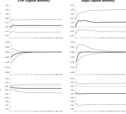
Briefly, the main findings are as follows: (i) In concordance with existing literature, fiscal multipliers are larger in advanced economies, when public debt is low, at a high level of financial development, in a financial crisis, and during business cycle downturns; (ii) However, contrary to conventional wisdom, fiscal multipliers in countries that are relatively open to trade are not smaller than their closed counterparts. Although there is demand leakage through imports in open economies, the increase in private consumption more than offsets the decline in net exports; (iii) Fiscal multipliers are also not smaller in countries with relatively high international capital mobility, contradicting the predictions of the traditional Mundell-Fleming model. This can be explained by the shaper depreciation of the real exchange rate and the relaxation in monetary policy; (iv) In addition, fiscal multipliers in flexible exchange rate regimes are not smaller than fixed regimes. There is no evidence of monetary policy accommodation under fixed exchange rate regimes, contrary to what the Mundell-Fleming model would suggest. Moreover, under flexible exchange rate regimes the real exchange rate does not appreciate in response to an increase in government spending; (v) The qualitative findings in Ilzetzki et al. (2013) can be obtained by using annual data for their country sample in both the standard structural vector autoregression (SVAR) and sign restriction identification schemes. This suggests that the results in Ilzetzki et al. (2013) are not sensitive to data frequency and the identification methodology, but are driven by the country sample; and (vi) The key to understanding the divergence of the results surrounding the three measures of openness—trade openness, capital mobility, and exchange rate flexibility—are the response of the real exchange rate and the degree of monetary policy accommodation. This underscores the importance of fiscal and monetary policy interactions in determining the size of fiscal multipliers.

(36)

15

2.2 Macroeconomic effects of fiscal policy: theory and empirics

It is instructive to briefly discuss what theory says about the expected consequences of a fiscal expansion. In the context of the closed economy textbook IS-LM model, an increase in government spending shifts the IS curve to the right. Labour demand increases, resulting in higher real wages and a higher level of output and consumption. Interest rates also rise, which can crowd out investment. The open economy counterpart to the IS-LM model is the Mundell-Fleming model. Under a flexible exchange rate regime, a fiscal expansion raises real interest rates and the nominal exchange rate appreciates. With nominal price sluggishness, the real exchange rate therefore appreciates and the trade balance deteriorates, thus limiting the expansionary effects of higher government spending. If there is perfect capital mobility, the resulting reduction in net exports completely offsets the fiscal expansion. In contrast, under a fixed exchange rate regime the monetary authority increases money supply to keep the exchange rate fixed, resulting in higher output while net exports remain unchanged.

These traditional models do not account for inter-temporal aspects of fiscal expansions. There are trade-offs between the short-run benefits and additional public debt accumulation that requires higher future tax increases or spending reductions. In neoclassical RBC models (e.g., Baxter and King, 1993) the discounted value of future tax rises generates a negative wealth effect that induces individuals to reduce private consumption and leisure. Labour supply increases, real wages fall and there is an increase in output. The increase in employment raises the marginal product of capital and attracts more private investment. Likewise, in a neoclassical open economy model setting (e.g., Baxter, 1995), the above dynamics are also at work. In addition, a fiscal expansion, which is typically more intensive in home-produced non-traded goods, leads to a real exchange rate appreciation (i.e., price of domestic goods increases relative to foreign goods) and a deterioration in the trade balance.

(37)

16

is typically followed by an increase in private consumption (e.g., Fatás and Mihov, 2001; Blanchard and Perotti, 2002) and a real exchange rate depreciation (e.g., Kim and Roubini, 2008; Monacelli and Perotti, 2010; Ravn et al., 2012).

Several approaches have been proposed to account for these empirical ‘puzzles’. Linnemann (2006) introduces non-separability of consumption and leisure in the household utility function. Due to consumption and leisure being substitutes, the reduction in leisure as a consequence of fiscal expansion increases the marginal utility of consumption. This positive effect on consumption could offset the negative wealth effect, and is more likely the higher the degree of substitutability between consumption and leisure and the lower the inter-temporal rate of substitution. Bouakez and Rebei (2007) introduce preferences which depend on private and public spending, along with habit formation. The complementarities between private and government consumption enable the model to generate a positive response of private consumption to a government spending shock. Galí et al. (2007) introduce non-Ricardian (rule-of-thumb) households that consume their current disposable income. If this group of consumers is sufficiently large, the positive effect on current consumption could offset the negative wealth effect of optimizing households.

On the real exchange rate depreciation puzzle, Kollmann (2010) emphasizes that the real exchange rate can depreciate if government spending shocks are persistent and international financial markets are incomplete. Corsetti et al. (2012a) show that if government spending contributes to debt stabilization, fiscal expansion today induces expectations of future spending cuts; long-run real interest rates therefore do not rise and the real exchange rate depreciates. Ravn et al. (2012) reconcile the puzzle by introducing deep-habit formation, in which an increase in domestic aggregate demand provides firms with incentives to lower markups. The decline in domestic markups relative to foreign markups leads to a real exchange rate depreciation.

(38)

17

2.2.1 Economic development

Studies on advanced economies typically produce fiscal multipliers between zero and one in the first year (see Batini et al., 2014). Kraay (2012), Estevão and Samaké (2013), and Ilzetzki et al. (2013) find that fiscal multipliers in advanced economies are larger than developing countries. Among the reasons put forth to explain why fiscal multipliers tend to be smaller in developing countries are implementation lags and weaker management in public spending and higher precautionary savings owing to instability and uncertainty.2

2.2.2 Trade openness

According to Keynesian models, government spending has maximum potency when the effects are contained in the domestic economy. Fiscal multipliers are therefore expected to be smaller in open economies, which have a higher propensity to import, as a fiscal expansion leads to demand leakage through imports instead of an increase in domestic production to satisfy the increase in aggregate demand. The findings of Ilzetzki et al. (2013) support this conventional view; fiscal multipliers are smaller in countries which are relatively open to trade. They find similar results even with alternative definitions of trade openness such as using tariff rates and economy size.

2.2.3 Capital mobility

Another important dimension of globalization is increasing financial integration and the reduction of barriers to international capital flows. However, the role of capital mobility has attracted considerably less attention as a determinant of the size of the fiscal multiplier. According to the traditional Mundell-Fleming model, the effectiveness of fiscal policy is an inverse function of the degree of international capital mobility. Capital mobility gives rise to an exchange-rate induced crowding-out effect, diminishing the efficacy of fiscal stimuli. This core result also holds in open economy general equilibrium models with micro foundations (e.g., Sutherland, 1996).

2

Institutional factors could also be important in determining the effectiveness of fiscal policy. Developing

countries tend to have lower institutional quality; to some extent, economic development captures the

(39)

18

Contrary to conventional wisdom, Pierdzioch (2004) shows that a high degree of capital mobility can also increase the effectiveness of fiscal policy. He emphasizes the importance of taking into account the interaction between fiscal and monetary policy to understand the transmission of fiscal shocks. Adding a richer specification of the monetary policy rule into the model of Sutherland (1996), he finds that the output effect of a fiscal policy shock increases in the degree of capital mobility under nominal income targeting but the opposite is observed if the central bank keeps money supply constant.

In addition, according to the optimizing consumption-smoothing view, a high degree of capital mobility allows forward-looking agents to smooth consumption through the dynamics of the current account. From this inter-temporal standpoint, lower impediments to capital movements allow the current account to act as a buffer in the face of shocks; hence the negative wealth effect is smaller and fiscal multipliers could be larger.

2.2.4 Exchange rate regime

As discussed earlier, the Mundell-Fleming model predicts that a fiscal expansion is ineffective under flexible exchange rates as it leads to an exchange rate appreciation which crowds out net exports. In contrast, fiscal policy is effective under fixed exchange rates since monetary expansion keeps the exchange rate unchanged. Monetary policy accommodation therefore plays a crucial role. The findings in Corsetti et al. (2012b), Born et al. (2013), and Ilzetzki et al. (2013) provide support for this traditional view.

(40)

19

argument holds only when the monetary policy pursued is an exogenous money supply rule. If the monetary policy is based on inflation targeting instead, the picture is reversed. In this case, under a flexible exchange rate regime the monetary authority reacts to inflationary pressures of the fiscal expansion by raising interest rates. The resulting effect could be a smaller multiplier compared to a fixed regime. Based on these findings, Dellas et al. (2005) emphasize that one should not expect to see a systematic relationship between exchange rate flexibility and the size of fiscal multipliers in cross-country studies, unless one also conditions for the domestic monetary policy rule.

2.2.5 Debt burden

When public debt is high, forward-looking agents anticipate that they are more likely to pay higher taxes sooner and therefore increase their savings (Sutherland, 1997). The anticipation of such an adjustment could have a contractionary effect which could offset the expansionary impact of higher government spending today. In a model with heterogeneous households, Perotti (1999) shows that when the debt level is high, distortionary taxes amplify the negative wealth effects of unconstrained households which could outweigh the positive effects of a fiscal expansion on the income and consumption of credit-constrained households.

The few empirical studies thus far give credence to the notion that high debt is harmful. Kirchner et al. (2010) find evidence of higher debt-to-GDP ratios negatively affecting long-term fiscal multipliers in the Euro Area. Ilzetzki et al. (2013) estimate long-run fiscal multipliers of -3 in episodes of high government debt.

2.2.6 Financial development

(41)

20

a more developed financial sector, hence, fiscal multipliers could be larger. The other aspect relates to the cost of government borrowing. In countries with limited access to financial markets, governments can only issue debt to finance deficits at high interest rates, which diminishes the effectiveness of fiscal policy. On the other hand, there is also the possibility that governments can issue debt to a captive domestic market in financially depressed countries, which increases the size of fiscal multipliers.

2.2.7 Financial crisis

In a financial crisis the proportion of credit-constrained agents typically increases, implying larger fiscal multipliers during such episodes. This can be seen in the New Keynesian model of Galí et al. (2007), whereby an increase in government spending increases the consumption demand of credit-constrained households, which reinforces the expansionary effects of fiscal policy. Using a panel of OECD countries, Corsetti et al. (2012b) find that fiscal multipliers are about two times larger during a financial crisis. However, Romer and Romer (2015) find that output declines are relatively moderate, depending on the severity and persistence of the distress.

In the case of interest rates reaching the zero lower bound, which is the prevailing economic environment in the aftermath of the global financial crisis, fiscal stimulus is then fully accommodated since the policy rate remains unchanged at zero. Fiscal multipliers can be unusually high, between two and four (see Eggertsson, 2010; Christiano et al., 2011; Woodford, 2011).

2.2.8 State of the business cycle

(42)

21

2.3 Estimating fiscal multipliers

Empirically, estimating fiscal multipliers faces some challenges. Fiscal multipliers measure the change in output in response to an exogenous change in fiscal policy. Identifying exogenous shocks is difficult due to reverse causality—government spending affects GDP, but GDP also affects government spending. There are generally two approaches to identify fiscal spending shocks in the literature.3

The second is based on the SVAR approach to model dynamic relationships of endogenous variables (e.g., Fatás and Mihov, 2001; Blanchard and Perotti, 2002; Perotti, 2005). Blanchard and Perotti (2002) identify fiscal spending shocks by assuming that government expenditure does not respond to GDP in the same quarter; hence, exogenous fiscal policy can be isolated by using quarterly data and ordering government expenditure before GDP. Another empirical challenge is the lack of high-frequency and long time series data, especially for developing countries. Many studies rely on the Blanchard and Perotti (2002) identification method which necessitates the use of quarterly data if the fiscal shocks are to be considered credible.

The first is based on the ‘natural experiment’ or narrative approach in identifying exogenous variation by using military spending (e.g., Ramey and Shapiro, 1998; Edelberg et al., 1999; Burnside et al., 2004; Barro and Redlick, 2011). The main idea behind this approach is that military spending is determined by wars and can therefore be treated as exogenous. However, this argument is invalidated in many developing countries since wars could be due to prevailing economic conditions, thus making military spending endogenous to the economy. Another criticism points to the possibility of other fiscal shocks occurring around the same time, which raises doubts on the identification of military build-ups.

Nevertheless, there are studies that apply the SVAR approach to lower frequency data. For instance, Beetsma et al. (2008) justify that the use of annual data provides several advantages. First, the identified fiscal shocks using annual data may correspond more closely to actual shocks since government expenditure decisions typically follow an annual cycle. Second, the role of anticipation effects is less relevant as a given shock is less likely to be anticipated one year beforehand. Anticipation effects are usually

3

Only empirical estimation approaches are discussed here. Batini et al. (2014) provides a summary on the

(43)

22

present in VAR models estimated with quarterly data (Ramey, 2011). Third, seasonality effects are less important in annual data.

Recent methodological advances utilize sign restrictions to identify fiscal shocks (e.g., Canova and Pappa, 2007; Mountford and Uhlig, 2009; Dungey and Fry, 2009; Pappa, 2009).4

2.4 Data and methodology

As Pappa (2009) notes, the sign restriction approach offers a few advantages over the conventional SVAR approach: it is theory-based, applicable to data with any frequency, and largely solves the problem of endogeneity and predictability of fiscal variables.

2.4.1 Identifying a shock to fiscal spending

Existing studies typically require quarterly data to identify a fiscal spending shock, which narrows the scope of analysis to advanced economies. Although Ilzetzki et al. (2013) use a larger quarterly data set, their sample is confined mainly to advanced and larger developing (emerging) economies. To examine the robustness of the empirical findings in Ilzetzki et al. (2013) for a larger country sample, especially including developing countries, an alternative approach to credibly identify a shock to fiscal spending is required since only annual data is available. The sign restriction methodology comes in handy in this context.

I adopt the theoretical restrictions in Pappa (2009) to identify a shock to fiscal spending. Pappa (2009) shows that in both prototypical flexible price RBC and sticky price New Keynesian models, a fiscal spending shock increases output and the deficit on impact. These responses are robust for a wide range of parameterizations. Furthermore, other shocks cannot produce the same responses on impact. In particular, technology, labour supply, and monetary shocks decrease the fiscal deficit at least on impact. A shock to fiscal spending is therefore identified by employing the sign restrictions in Table 2.1.

4

The sign restriction methodology is originally developed by Faust (1998), Canova and De Nicolò

(44)

23

Table 2.1 Sign restrictions to identify a shock to fiscal spending

Government

consumption GDP Fiscal balance

Real exchange rate

Fiscal spending

shock > 0 > 0 < 0

Notes: Sign restrictions hold only on impact.

It is important to note that the fiscal policy analysed here is a deficit-spending scenario. Tax cuts can also increase output and the deficit. However, a deficit-financed tax cut fiscal policy does not usually lead to an increase in government expenditure. One way to ensure the identified shock is not polluted by tax cuts is to add another restriction that requires tax revenues to be zero or positive. Including this additional sign restriction does not change any of the results in the paper but requires estimating a larger VAR.5

A related issue in identifying a single shock is the ‘multiple shocks problem’ as highlighted in Fry and Pagan (2011), i.e., the set of responses could have been generated by more than one potential shock and there is insufficient information to discriminate among the shocks. A possible solution is to reject all the draws for which the unidentified shocks deliver impulse responses that are consistent with the signs of the identified shock. However, potentially some useful information is lost when such draws are discarded. An alternative solution, which is used in this paper, is to apply magnitude restrictions to disentangle the shocks. For instance, if two shocks have the same set of impulse responses, the shock in which the response of government consumption is larger is considered as a fiscal spending shock. This is similar to the approach taken in Peersman (2005) and Dungey and Fry (2009).

2.4.2 The sign restriction approach

A structural panel VAR model of 𝑚 variables can be represented as:

5

Government revenue is used as a proxy for tax revenue since long time series data on tax revenue is not

available for many countries. Adding government revenue in the VAR decreases the sample size by about

(45)

24

𝐵0𝑌𝑖,𝑡= � 𝐵𝑘𝑌𝑖,𝑡−𝑘+𝜀𝑖,𝑡 𝐾

𝑘=1

, 𝑡= 1, … ,𝑇 (2.1)

where 𝑌_𝑖,𝑡 is a vector of the 𝑚 endogenous variables for country 𝑖 in year 𝑡, 𝐾 is the lag length, 𝐵₀ is the contemporaneous coefficient vector of 𝑌_𝑖,𝑡, 𝐵_𝑘 is a 𝑚 x 𝑚 matrix of coefficient parameters, and 𝜀_𝑖,𝑡 denotes the ‘fundamental’ or structural macroeconomic shocks.

The reduced form representation of (2.1) is given by:

𝑌𝑖,𝑡 = � 𝐴𝑘𝑌𝑖,𝑡−𝑘+𝑒𝑖,𝑡 𝐾

𝑘=1

, 𝑡= 1, … ,𝑇 (2.2)

where 𝐴_𝑘 =𝐵_𝑜−1𝐵_𝑘, and 𝑒_𝑡 =𝐵_𝑜−1𝜀_𝑖,𝑡 are the reduced-form residuals with 𝑚 x 𝑚 variance-covariance matrix 𝐸�𝑒_𝑖,𝑡𝑒_𝑖,𝑡′ �= Σ.

Given a set of sign restrictions imposed on the impulse responses, the sign restriction method searches over the space of possible impulse vectors to find those satisfying the criteria. To construct structural impulse response functions, an estimate of the matrix 𝐵�_𝑜−1 in 𝑒_𝑡 =𝐵�_𝑜−1𝜀_𝑡 is required. Let 𝛴 =𝑃𝛬𝑃′ and 𝐵= 𝑃Λ0.5 such that 𝐵 satisfies 𝐵𝐵′ =𝛴. Then 𝐵�_𝑜−1 =𝐵𝐷 also satisfies 𝐵�_𝑜−1�𝐵�_𝑜−1�′ = Σ for any orthogonal matrix 𝐷. The sign restrictions procedure used in this paper is based on the Householder transformation (see Rubio-Ramírez et al., 2010) and involves the following steps:

(i) Draw an independent standard normal 𝑚 x 𝑚 matrix 𝑋 and derive the QR decomposition of 𝑋 such that 𝑋 =𝑄𝑅 and 𝑄𝑄′=𝐼_𝑚;

(ii) Let 𝐷 = 𝑄′. Compute the impulse responses using the orthogonalization

𝐵�𝑜−1 =𝐵𝐷 and keep the structural models that satisfy the sign restrictions;

(iii) Repeat the first two steps until the number of admissible structural models reaches the desired number;

(iv) Sort the structural models and select the one whose impulse responses are closest to the median values (median target method; see Fry and Pagan, 2011).6

6

Since each structural model represents a different relationship between variables in the VAR, there

exists a ‘multiple models problem’ as discussed in Fry and Pagan (2011). Presenting the median as a