Time Based Change Visualization Techniques Survey

ISSN: 1816-949X

© Medwell Journals, 2019

Time-Based Change Visualization Techniques Survey

Ales Komarek, Jakub Pavlik and Vladimir Sobeslav

Faculty of Informatics and Management, University of Hradec Kralove,

Hradec Kralove, Czech Republic

Abstract: Sets of numerical values changing over time are one of the most common forms of recorded data. Time-varying phenomena are essential to many areas of human activity and there is often a need to simultaneously display or compare a large number of time series data. Visualizations that improve the speed and accuracy with which humans can read and compare time-varying data are of great practical benefit. Effective presentation of multiple time series is one of the basic problems in visualization research: increasing the amount of data with which human operators can effectively work. This study surveys visualization techniques for time-series data with their major pattern and quantitative qualities compared. All covered visualizations are implemented in ‘Visualization Laboratory’ project and use common format to handle time-series data.

Key words: Time series, quantitative data, visualization, chart, qualities, presentation

INTRODUCTION

Time-series visualizations improve the speed and accuracy with which data can be compared and proper displaying contrast of various time-varying data are of great practical benefit. Toward this aim, researchers and designers have devised design guidelines and visualization techniques for making more effective use of display space. Edward (1986) advises visualization designers to maximize data density (number of data represented by charts) and researchers regularly promote visualization techniques (Aigner et al., 2007; Aigner, 2006; Muller and Schumann, 2003) that provide good “space-filling” properties. Time-series visualizations find usage in many fields of human endeavor, this include for example: scientific fields (temperatures, pollution levels, electric potentials), financial sector (stock prices, exchange rates) or public policy (crime rates, unemployment rates).

Such approaches excel at increasing the amount of information that can be encoded within a display (Aigner, 2006). However, increased data density does not necessarily imply improved graphical perception for visualization viewers. We compare the qualities of commonly used visualization techniques. These time series qualities are the following:

Time series: Number of time series displayed in single visualization layout.

Time intervals: Number of time intervals or data points displayed in single visualization layout.

Value domains: Possible value domains for data in selected visualization layout. Values may be continuous, discrete or given other dictionary.

These qualities provide recommended guidelines to keep the high readability level of the surveyed visualization techniques.

Along the quantitative qualities, we can find pattern-oriented qualities as well (Muller and Schumann, 2003). Patterns provide basic classification for the visualization techniques and show ho appropriate these are for certain use cases. Basic patterns are summarized in the following list.

Comparisons: These visualization techniques help show the differences or similarities between displayed numerical values.

Distribution: These visualization techniques display frequency how data spread out over a given interval of time.

Patterns: These visualization techniques reveal forms or patterns in the time series data to give it further meaning. Proportions: These visualization techniques that use size or area to show differences or similarities between values or to a whole.

These time series visualization qualities are further evaluated in chapter “Time series visualization comparison”.

A team from tcp cloud a. s. and University of Hradec Kralove carries out a “Visualization Laboratory” project to demonstrate the possibilities of modern visualization Corresponding Author: Ales Komarek, Faculty of Informatics and Management, University of Hradec Kralove, Hradec Kralove,

techniques. The activities of this study includes the state-of- the-art analysis of time-series visualizations and the selection of the appropriate techniques for carrying out the testing. The section 3; compares quantitative and pattern-oriented qualities for all covered visualization techniques. The section 4; describes the testbed environment and the fundamental technologies used to carry on the “Visualization Laboratory” project. Final section covers results coming out of the PoC project.

STATE-OF-THE-ART VISUALIZATION TECHNIQUES

This chapter shows various techniques of time-series visualizations. Following list of visualizations summarizes modern visualization techniques. This list does not cover relational based visualizations which are covered in our previous paper (Muller and Schumann, 2003).

Line chart: Line charts are used to display quantitative value over a continuous time interval (Tominski et al., 2004). When grouped with other lines it can show trends and relationships. Line graphs help see how data has evolved over that period of time. Line graphs are drawn by first plotting data points on a Cartesian coordinate grid, then connecting a line between the points. Typically, the y-axis has a quantitative value while the x-axis has a time scale. Negative values can be displayed below the x-axis. Area chart: Area charts are form of line charts with the area below the line filled with a color (Tominski et al., 2004). Area charts are used to display the change of quantitative values over a time interval. They are most commonly used to show trends and relationships. Area charts are drawn by first plotting data points on a Cartesian coordinate grid, then line joins the points and finally the space below the completed line is filled. Horizon chart: Horizon charts are variation of area charts, that combine position and color to reduce vertical space requirements. They start as a standard area chart then the chart is folded into fixed numbers of bands. These bands overlap from lower numbers to higher and each band have a higher intensity of color. The negative values can be mirrored or vertically offsite. This technique was proposed by Heer et al. (2009).

Stacked area chart: Stacked area charts function in the same way as simple and grouped area charts, except that each following time series starts from the point left by the previous data series. The entire chart represents the sum of all the time series plotted. Stacked area charts use area to convey the values, so, they do not work for negative numbers. These charts are useful for comparing multiple variables changing over a time interval.

Radar chart: Radar charts are Polar version of area charts or grouped area charts. Each time point is provided an axis, that starts from the center. All axes are arranged radially with equal distances between each other. Circular grid lines are used as a guide. Each time series value is plotted to time axis and all complete time series is connected together to form a polygon. Having too many polygons in one radar chart makes it hard to read, confusing and too cluttered. Having too many time points creates too many axes and can also make the chart hard to read and complicated.

Grouped bar chart: Grouped bar charts are used when two or more-time series are plotted side-by-side on the time axis. The length of each bar is used to show discrete, numerical comparisons of each time series. Each series has assigned color in order to distinguish them. The use of grouped bar charts is usually to compare individual data points. The downside is that they become harder to read the more bars you have in one point on time axis. Bullet chart: Bullet chart works like a bar chart but is accompanied by extra visual elements to provide in more context. The main data value is encoded by length in main bar in the middle of the chart which is known as the “Feature Measure”. The line marker that runs perpendicular to the orientation of the graph is known as the “Comparative Measure” and is used as a target marker to compare against the feature measure value. So, if the main bar has passed the position of comparative measure, you know you’ve hit your goal. The segmented colored bars behind the feature measure are used to display qualitative range scores.

Histogram: A histogram visualizes the distribution of values from multiple times over a time period. Each bar in a histogram represents the tabulated frequency at each time interval. The total area of the histogram is equal to the number of time series. Histograms help give an estimate as to where values are concentrated what the extremes are and whether there are any gaps or unusual values. They are also give a rough view of probability distribution.

Stacked bar chart: Unlike a grouped bar chart which displays bars side-by-side, stacked bar charts segment their bars of multiple time series on top of each other. They are used to show how a larger category is divided into smaller categories and what ratio of each set has on the total amount.

that lengths can be easily misinterpreted. Each bar on the outside gets relatively longer to the previous, even if they represent the same value. This is because each bar has a different radius, so, the value each bar is by its angle. Radial bar chart: This type of chart is also known as star graph or rose chart. It uses a grid of concentric circles to plot bars on. Each circle represents a value on a scale, while the radial dividers are used for each time point. The lower values on the scale start from the center and increase with each concentric circle. If zero value is represented by any of the outer circles, negative values can be displayed.

Radial stacked bar chart: Radial stacked bar charts also known as Nightingale rose charts are created by stacking multiple bars in radial bar chart as in stacked bar chart. Each time point is given equal segment on the radial chart. The major flaw with Nightingale rose charts are that outer segments are given more emphasis because of their larger area size. This disproportionately represents increases in value.

Candlestick chart: Candlestick chart is used to describe value changes, usually in financial sector. Each “candlestick” represents on time step. It is a combination of line-chart and a bar-chart, each bar represents all four important pieces of information for that time step. Candlestick charts are most often used in technical analysis of equity and currency price patterns. They appear superficially similar to box plots but are unrelated. Open-high-low-close chart: An Open-High-Low-Close chart also known as OHLC chart is used to illustrate movements in the time series values over time. Each vertical line on the chart shows the value range (the highest and lowest values) over one-time point. Tick marks project from each side of the line indicating the opening values (e.g., for a daily bar chart this would be the starting values for that time point) on the left and the ending value for that time period on the right.

Calendar heat map: A heat map is a graphical representation of time-series data where the individual values are represented as colors and contained in a matrix (Wijk and Selow, 1999). Tree maps both often use a similar system of color-coding to represent the values taken by a variable in a hierarchy.

Pie chart: Pie charts help show proportions and between time series by dividing a circle into proportional segments (Heer and Robertson, 2007). Each arc length represents a proportion of each time series, the full circle represents the total sum of all the data at given time point. Pie charts are ideal for giving the reader a quick idea of the proportional distribution of the data.

Donut chart: A donut chart is form of pie chart with an empty area in the center (Heer and Robertson, 2007). With donut chart reader focuses more on reading the length of the arcs, rather than comparing the area proportions of individual slices. This help focusses more on the changes in overall values. Donut charts may use less space comparing to pie charts by having information displayed in their blank centers.

Dot matrix: Dot matrix also charts display discreet data in units of dots or icons, each colored to represent a particular time series value and grouped together in a matrix. They are used to give a quick overall of the distribution and proportions of each category in a data set and also to compare distribution and proportion across other datasets.

When only one variable/category is present and dots are all one color, a dot matrix chart works in the same way to proportional area chart.

Pictogram chart: Pictograph chart uses icons to give a more engaging overall view of small sets of discreet data. Time series are compared side-by-side in either columns or rows of icons. Each icon represents one unit or any number or units (e.g., each icon represents 10s). Using large numbers make values on the chart hard to count.

TIME SERIES VISUALIZATION COMPARISON

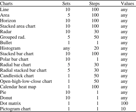
All surveyed visualization, we evaluated for the quantitative and pattern-oriented qualities using d3 library. The following Table 1 compares the quantitative qualities of selected time series visualization techniques. Pattern-oriented qualities: The following Table 2 compares the pattern-oriented qualities of selected time series visualization techniques.

Table 1: Quantitative qualities summary

Charts Sets Steps Values

Line 10 100 any

Area 5 100 any

Horizon 10 100 any

Stacked area chart 10 100 any

Radar 10 30 any

Grouped rad. 5 50 any

Bullet 1 1 any

Histogram any 20 any

Stacked bar chart 10 100 any

Polar bar chart 10 1 any

Radial bar chart 5 30 any

Radial stacked bar chart 5 30 any

Candlestick chart 1 50 any

Open-high-low-close chart 1 50 any

Calendar heat map 1 100 any

Pie 10 1 any

Donut 10 1 any

Dot matrix 1 1 100

Table 2: Pattern-oriented qualities summary

Charts Comparison Sets Steps Values

Line yes no no no

Area yes no no no

Horizon no no no no

Stacked area chart yes no no no

Radar yes no no no

Grouped rad. yes no yes no

Bullet yes no no no

Histogram yes no yes no

Stacked bar chart yes no no yes

Polar bar chart yes no no no

Radial bar chart yes no no no

Radial stacked bar chart yes no no yes

Candlestick chart no no no no

Open-high-low-close chart no no no no

Calendar heat map no no no no

Pie yes no no no

Donut yes no no no

Dot matrix yes no yes yes

Pictogram chart yes no yes no

PROOF-OF-CONCEPT TESTBED TECHNOLOGIES

Testbed environment is setup at cloud environment with following configuration: 1 application node-LeonardoCMS, PostgreSQL and 1 database node-graphite metric database, elastic search database. The core service is python application LeonardoCMS with d3.js components for each of the visualization. The data sources are graphite and elastic search databases with data inputters configured to populate them with sample data. D3.js is a JavaScript library used to show data (Bostock et al., 2011; Jain, 2014). It was created by Mike Bostock as project succeeding the Protovis visualization library (Bostock and Heer, 2009). It has multiple visualization use cases available in public domain. The nvd3 library is used to power many of the quantitative visualizations.

Leonardo CMS is a powerful content management system aimed on extensibility and has multiple functional modules in basic setup, making it ideal tool to include domain specific module. We have extended the platform with following modules:

Quantitative analysis is effective presentation of multiple time series is one of the basic problems in visualization research: increasing the amount of data with which human operators can effectively work. This model surveys and implements various methods suitable for visualizing the time-series data, both current and historical. Visualizations that belong to this module are part of this study. For example, visualization displayed in Fig. 1 is stacked area chart visualization in several modifications.

Relational analysis are visualizations for all kinds of networks, complex systems and hierarchical graphs. This visualization is needed to analyze the complex relationships in various systems. It’s especially good for revealing the underlying structures of associations between objects and for graph analysis.

Fig. 1: Quantitative time-series visualization sample: stacked area chart

Temporal analysis deals with our understanding of time and temporal patterns often depends on the lens through which we view it. Data visualizations provide a set of lenses through which we can view time from different perspectives.

Geospatial analysis emphasizes knowledge construction over knowledge storage or information transmission. To do this, geographical visualization communicates geospatial information in ways that, when combined with human understanding, allow for data exploration and decision-making processes.

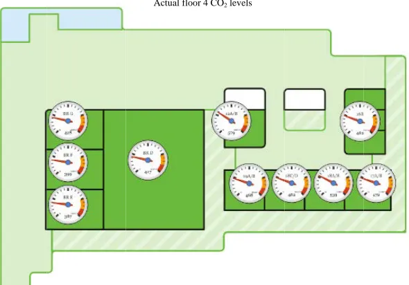
The utility of visualization can be boosted by combining multiple charts within one complex visualization. Figure 2 and 3 shows, combination of vector floorplan with quantitative visualization of selected metrics. To further the effect, dashboards can serve as container for multiple charts to present various views on given system.

Fig. 2: System charts can combine multiple standalone charts

Fig. 3: Combination of several visualizations in dashboard for complete system view CONCLUSION

Visualizations affect the speed and accuracy with which we can read and evaluate time-varying data. Researchers and designers have devised various visualization techniques for making more effective use of display space. However, there are limits to the number of data that can be presented at given time. This study shows PoC implementation of the most prominent time data visualization techniques and presents their limits comparison and basic pattern-based classification. The Cartesian grid based charts generally support more

metrics and time samples than those based on polar grid. The horizon chart can support multiple metrics while retaining perfect readability.

complex visualizations multi-domain (service metrics, services relation metrics, states etc.) metadata needs to be supplied and declaration can be more time consuming.

ACKNOWLEDGEMENTS

This research and the contribution were also supported by project “Smart Solutions for Ubiquitous Computing Environments” FIM, University of Hradec Kralove, Czech Republic (under ID: UHK-FIM-SP-2016-2102).

REFERENCES

Aigner, W., 2006. Visualizing time and time-oriented information: Challenges and conceptual design. Ph.D Thesis, Vienna University of Technology, Vienna, Austria.

Aigner, W., S. Miksch, W. Muller, H. Schumann and C. Tominski, 2007. Visualizing time-oriented data-a systematic view. Comput. Graphics, 31: 401-409. Bostock, M. and J. Heer, 2009. Protovis: A graphical

toolkit for visualization. IEEE. Trans. Visual. Comput. Graphics, 15: 1121-1128.

Bostock, M., V. Ogievetsky and J. Heer, 2011. D³ data-driven documents. IEEE. Trans. Visual. Comput. Graphics, 17: 2301-2309.

Edward, R.T., 1986. The Visual Display of Quantitative Information. Graphics Press, Cheshire, Connecticut,. Heer, J. and G. Robertson, 2007. Animated transitions in statistical data graphics. IEEE. Trans. Visual. Comput. Graphics, 13: 1240-1247.

Heer, J., N. Kong and M. Agrawala, 2009. Sizing the horizon: The effects of chart size and layering on the graphical perception of time series visualizations. Proceedings of the SIGCHI Conference on Human Factors in Computing Systems, April 4-9, 2009, ACM, Boston, Massachusetts, ISBN:978-1-60558-246-7, pp: 1303-1312.

Jain, A., 2014. Data visualization with the D3 JS JavaScript library. J. Comput. Sci. Colleges, 30: 139-141.

Muller, W. and H. Schumann, 2003. Visualization methods for time-dependent data-an overview. Proceedings of the Conference on Winter Simulation, December 7-10, 2003, IEEE, Germany, ISBN:0-7803-8131-9, pp: 737-745.

Tominski, C., J. Abello and H. Schumann, 2004. Axes-based visualizations with radial layouts. Proceedings of the 2004 ACM Symposium on Applied Computing, March 14-17, 2004, ACM, Nicosia, Cyprus, ISBN: 1-58113-812-1, pp: 1242-1247.