Primon : the implementation of a software monitor : a thesis presented in partial fulfilment of the requirements for the degree of Master of Science in Computer Science

PRIMON:

The Implementation of a Software Monitor

by

Anthony James McGregor

A thesis presented in partial fulfilment of the requirements for the degree of

Master of Science in Computer Science

at

Massey University

ABSTRACT

ACKNOWLEDGEMENTS

I would like to thank,

Tom Docker, my supervisor, particualarly for his efforts while criticising the many drafts of this thesis, and

Table of Contents

Introduction ...•...•.•••....•.•.••..••...•...•.•.•..•••••••••••• 1 2 An introduction to computer performance evaluation •••••••••••••••••• 9 2. 1 Monitors •••.•••••••••••.••••••••.•••••••••••••.•••••••••••••••• 12 2.2 Models ••••••••••••••••••••••••••.•••••••••••••••••••••••••••••• 15 3 The

3.

1 3.2

3.3

principles of software monitoring •••••••••••••••••••••••••••••• 25 The structure of software monitors ••••••••••••••••••••••••••••• 25 Performance indices ....••...•...••.•••....••. 27

Measuring disciplines •••••••••••••••••••••••••••••••••••••••••• 28

3.3.1 Event trapping•••••••••••••••••••••••••••••••••••••••••••30 3.3.1.1 Collecting the data •••••••••••••••••••••••••••••• 31 3.3.1.2 Recording the data ••••••••••••••••••••••••••••••• 31 3.3.1.3 Problems with event trapping ••••••••••••••••••••• 33 3.3.1.3.1 Access •••••••••••••••••••••••••••••••••••••• 33 3.3.1.3.2 Overheads ••••••••••••••••••••••••••••••••••• 34

3.3.1.3.3 Sensitivity •.•••••••••••.••••••••••••••••••• 34

3.3.2 (Random) 3.3.2.1

Sampling • ••••••••••••••••••••••••••••••••••••••• 35 Collecting the data •••••••••••••••••••••••••••••• 36 3.3.2.1.1 Collecting data by unit workloading ••••••••• 41 3.3.2.1.1.1 Advantages of unit workloads ••••••••••• 42 3.3.2.1.1.2 Disadvantage of unit workloads ••••••••• 43 3.3.2.2 Recording the data ••••••••••••••••••••••••••••••• 43 3.3.2.3 Advantages of random sampling •••••••••••••••••••• 44 3.3.2.3.1 Reducing distortion ••••••••••••••••••••••••• 44 3.3.2.3.2 Simplicity of installation •••••••••••••••••• 46 3.3.2.4 Problems with random sampling •••••••••••••••••••• 46 Reporting the results of monitoring •••••••••••••••••••••••••••• 47 3.4.1 Quoting the indices•·•••••••••••••••·••••••••••••••••••••48 3.4.2 Tables•••••·••••••••••··•••····•••••·•·••••·••••••••••••·48 3.4.3 Histograms••·••••••••••••••••••••••••••••••••••••••••••••49 3.4.4 Gantt profiles ••••••••••••••••••••••••••••••••••••••••••• 50 3.4.5 Kiviat graphs •••••••••••••••••••••••••••••••••••••••••••• 52

4.1.11 I/Os per second and page faults per second ••••••••••••••

64

4.1.12 I/0 trace•••••••••••••••••·••·••••••••••••••••••••••••••64 4.1.13 Page out trace•••••·•••••••••••·••••·•••·•••••••••••••••65 4.2 Inappropriate measures••••••••••••·••••••••••••••••••••••••••••65 4.2.1 Memory utilisation·••·••··•··••••••••••••••••••••••••••••65 4.2.2 Number of processes in memory••••••••••••••••••••••••••••65 4.3 Difficult measures···••••••••·•·•···•••·•••••••••••••••••••••••66 4.3.1 Number and source of interrupts••••••••••••••••••••••••••66

5 Primon•••••••••••••••••••••••••••••••••••••••••••••••••••••••••••••68 5.1 Features•••••••••••••••••••••••••••••••••••••••••••••••••••••••70 5.2 Development •••••••••••••••••••••••••••••••••••••••••••••••••••• 71 5.3 XREF•••••••••••••••••••••••••••••••••••••••••••••••••••••••••••74 5.4 The monitors .•••••••••.•••••.••••.•.••••••••••••••••••••••••••• 76

5.5

5.4.1 Interactive queue length monitor•••••••••••••••••••••••••77 5.4.1.1 Purpose•·••·•••••••••••••••••••••••••••••••••••••77 5.4.1.2 Background ••••••••••••••••••••••••••••••••••••••• 77 5.4.1.3 Implementation•••••••••••••••••••••••••••••••••••78 5.4.1.4 Distortion and integrity considerations •••••••••• 79 5.4.2 Validation.••••••••••••••••••••••••••••••••••••••••••••••79

5.4.2.1 Known variations•••••••••••••••••••••••••••••••••80 Batch

5.5.1 5.5.2

5.5.3

5.5.4

queue length monitor••·••••••••••••••••••••••••••••••••••81 Purpose••••••••••••••••••••••••••••••••••••••••••••••••••81 Implementation ••••••••••••••••••••••••••••••••••••••• ~ ••• 82 5.5.2.1 Reports••••••••••••••••••••••••••••••••••••••••••82

5.5.2.1.1 Distortion and integrity considerations ••••• 85 5.5.2.2 Validation ••••••••••••••••••••••••••••••••••••••• 86 5.5.2.2.1 Known variations.••••••••••·••••••••••••••••87 Disk activity monitor••••••••••••••••••••••••••••••••••••89 5.5.3.1 Purpose••••••••••••••••••••••••••••••••••••••••••89 5.5.3.2 Background•••••••••••••••••••••••••••••••••••••••90 5.5.3.3 Implementation ••••••••••••••••••••••••••••••••••• 91 5.5.3.4 Reports••••••••••••••••••••••••••••••••••••••••••94 5.5.3.5 Testing••••••••·•••••••••••••••••••••••••••••••••97

5.5.3.6

Validation •••••••••••••••••••••••••••••••••••••••

97

Relative availability monitor••••••••••••••••••••••••••••98 5.5.4.1 Purpose••••••••••••••••••••••••••••••••••••••••••98 5.5.4.2 Background ••••••••••••••••••••••••••••••••••••••• 98 5.5.4.3 Implementation••••••••••••••••••••••••••••••••••100 The sampler.•••••••••••••••••••••••••••••••101 5.5.4.3.1

5.5.4.3.1.1 The loosely coupled sampling

function•••••••••••••••••••••••••••••••••••••••101 5.5.4.3.1.2 The mini-benchmarks•••••••••••••••••••102 5.5.4.3.2 The reducer••••••••••••••••••••••••••••••••105 5.5.4.3.3 The plotter.•••••••••••••••••••••••••••••••105 5.5.4.3.4 The calibrator•••••••••••·•••••••••••••••••107 5.5.4.4 Testing•••••••••••••••••••••••••••••••••••••••••107 5.5.4.5 Validation •••••••••••••••••••••••••••••••••••••• 110 5.6 Extensions to Primon••••••••••••••••••••••••••••••••••••••••••112

5.6.3 Disk record positioning•·•••••••••••••••••••••••••••••••115 5.7 Evaluation of Primon••••••••••••••••••••••••••••••••••••••••••118 6 Conclusions ••••••••••••••••••••••••••••••••••••••••••••••••••••••• 120

1 Introduction

Computer Performance Evaluation (CPE) has developed both as an

academic and an applied subject of considerable importance, as

witnessed by its mention in Discussion Paper 3 for the recent Brownlie

Committee report [BROW82]. As an applied discipline CPE is used

primarily in the areas of

o computer design and development

o capacity planning and

o system tuning.

A need for access to CPE tools can be identified when administering

most computer systems and to this end a range of tools is available on

most (large) computers. Prime computers are a notable exception and

several groups involved with Prime equipment have shown a desire for

access to CPE tools. These groups include computer centres, who wish

to improve the performance of the computer systems under their

control, researchers in CPE, and teaching staff who wish to

demonstrate the use of performance evaluation.

This thesis reports on the implementation of one such tool called

Primon. We begin in chapters two and three by discussing CPE in

2 An introduction to computer performance evaluation

The performance evaluation of computer systems has become widespread because of the high cost and complex nature of modern computers.

As an example of the use of CPE consider a computer system operated by Superior Operational Software (SOS), a fictitious software company writing system software for Prlme computers. The system functions well until the number of interactive users exceeds a threshold. The System Administrator is faced with the task of raising this threshold, while remaining within a strict capital budget.

I

V

Performance Problem

I

l(CPE Study)

I

I

A

---.

I V

Problem Identified Problem not Identified

I

I

I

I

I

I

I

I

I

(problem insoluble) V

.---A--->

Problem not solved (solution I

available)!

I

j(Tuning / Capacity Planning)

I

V

Problem solved.

Example use of CPE Fig 2.1

This type of scenario is common but is by no means the only use of

CPE. Performance questions also arise when designing new systems, or

when choosing a new or replacement system. Hopefully a company

installing a computer system for the first time will want to be

satisfied that the proposed system will have sufficient capacity to

process the workload within an acceptable time frame. A manufacturer

designing a new machine may have specified design criteria which

include instruction execution rate improvements over a previous model.

Performance Evaluation is used in these situations as well.

has led to a range of tools to be developed for use in CPE. Many of

these tools have been developed for a particular CfE project, while

others are Operations Research techniques. Fig 2.2, and the rest of

this chapter, describe some of the more common techniques and their

relationships to one another. Other categorizations are possible and

some techniques are also known by other names.

A specific monitoring tool could be made up of more than one of these

techniques. For an example see the hybrid model of [SCHW78].

Computer Performance Evaluation Techniques

Monitoring

I

I

.---+--A---.

Software Hybrid Hardware

A

I

I

A

I

Modelling

I

A

Benchmark Predictive

.---

---.

A

.--- ---.

Traps Sampling Accounting Empirical

The CPE tree Fig 2.2

Queueing Network

I

[image:11.559.47.497.318.545.2]

2.1 Monitors

To continue the case of SOS Software, the System Administrator

believes that the disk drives are the cause of the problem and

instructs his staff to make changes to the operating system so that

it will monitor the number of I/Os and the number of users logged

onto the machine. This data will allow a plot of I/O activity

against the number of uses to be drawn. He also arranges for a

specialised micro-computer to be connected to the CPU and to each

disk drive. Every few milliseconds this computer monitors the state,

busy or idle, of each device and produces a plot of the device

utilisation against the time of day. It is hoped that on analysis

this data will show whether there is a relationship between the

interactive threshold and the I/O rate.

In general monitoring tools collect, and present, data from an

existing computer system. They are normally categorized by the

method(s) used to collect the measurement data.

The micro-computer used by SOS to collect device utilisations is an

example of a hardware monitor. Such devices are typically

specialised small computers, and are connected to the system to be

measured by passive electronic probes. This allows data to be

collected without the need to alter the way the host (or target)

system functions. The probes may be attached to the backplane of the

hardware monitoring can be found in [CARL76a] and [CARL76b].

Pieces of monitoring code that are executed by the system to be

measured, such as the operating system modification made by SOS, are

called software monitors. In chapter 3 we consider the ways that

software monitors collect data, particularly event trapping, where

code is inserted into the operating system (the case with the SOS

software monitor), and sampling, where an extra process is introduced

to take samples of the data of interest. We also consider methods of

recording the data that has been collected and methods of presenting

the data recorded. Data presentation is an important part of any

monitoring exercise.

A special type of software monitor found on most computers is the

accounting system, which collects and records data on the resources

used by individual users for charging purposes. This data is

periodically collated into a billing report. While the primary

function of this monitor is to allow a charging policy to be

implemented, data is often recorded which can be of interest to the

performance analyst [COX76].

A third class, called hybrid monitors because they are made up of a

combination of hardware and software, is often given theoretical

consideration. In practice hybrid monitors are not often implemented

as such, but the hardware and software of a computer system may be

designed with some consideration of further monitoring requirements.

event. It may then be possible to extract the counts from outside

the system using a hardware monitor; alternatively the hardware may

keep some performance index in a register which a software monitor

could read.

There are fundamental differences between hardware and software

monitors as described in following Table.

Software Hardware

---+---Pieces of code executed by Attached electrically. target machine.

Specifically designed for the target machine.

Introduces new overheads to target machine begin measured.

Simple to rerun.

No access to some hardware measures.

Easily measures software resources.

Less expensive.

Software damage may occur

(software and data held on the system may be corrupted).

Most of the information

required is about the system software.

Generalised hardware is available but the connection points and data reduction techniques are specific to each target machine.

Adds no new overheads.

Reattaching probes or attaching to a new machine takes time and skill.

Can measure most hardware components, except those

implemented within a single chip.

Cannot realistically measure most software resources.

More expensive.

Hardware damage may occur.

Most of the information required is about the system hardware. ·

It is interesting to consider the effects that the major trends in

hardware development will have on this comparison. The first trend

is the increase in power of hardware. As the number of instructions executed each second increases, the percentage overhead introduced by

adding a constant number of instructions (to implement a software

monitor) will get lower. The second trend is for hardware to be

implemented in ever fewer physical devices. As the number of

cabinets, the number of boards and the number of chips all decrease

there will be fewer places where a hardware monitor can be connected.

If these trends continue software monitors will become more

attractive at the expense of hardware monitors, although it is likely

that both will remain necessary to achieve all desired measurements.

The data derived from a monitor may be used directly in making tuning

or capacity planning decisions. It is increasingly more common,

however, for it to be used as source data in a model of the system.

For example the mean I/0 time, although useful in itself, could also

form part of the input data to a queueing network model, such as

QNEMU [LADY84].

2.2 Models

Returning to our example system, as a result of the monitoring

exercise the System Administrator at SOS finds that paging disk

utilisation is extremely high at the time the system degrades, and

system is thrashing (paging-bound) and considers the possibility of

adding some extra memory to the system. To lower the possibility of

purchasing this memory and being disappointed with the results, he

attempts to predict what improvement is likely to result from the

extra memory. He assembles a group of typical programs to form a

benchmark and runs them on the system overnight when no other users

have access. During the running of the benchmark the hardware

monitor is used to measure the CPU utilisation. Over successive

nights he re-runs the programs with less and less memory on the

machine, and enters all the results onto a graph showing the CPU

utilisation against the number of pages of memory in the system.

Finally he extrapolates (by eye) the trend shown on the graph by

assuming a 10% (+5)% increase in available pages if he adds one extra

CPU Utilisation I

I

/ / I I+ / I I + /

I

I

I II

,,

/

1

/ / / / /

+

I ....- I

/ I

/ ,

+/ I

/ I

-

-

-

-.__ _ _ _ _._ _ _ _ _ _ _ _._ _ _ ..._ _ _ _ _ _ _ _ _ _ _ _ _ _ _ _ ~ Pages o

' - - - ' Memory

Extra Memory Board

SOS's CPU utilisation plot Fig 2.3

Computer systems are both complex and expensive. The complexity is increased by the non-deterministic nature of the workload processed by most interactive systems. As a result:

o measurements are generally non-reproducible. difficulties when

- comparing machines

- creating acceptance criteria

This causes

o The behaviour of the system in total is hard to interpret.

As well as these, for a large number of interactive systems,

o The CPE team cannot easily get exclusive access to the computer.

These problems can be addressed to varying degrees by experimenting on a simplified model of the system, its workload, or both.

+---+

I

Transaction generator

I

+---+

I I I I I I I I I

I I I I I I I I I

I I I I I I I I I

<---Terminal lines

(may be multiplexed)

V V V V V V V V V

+---+

I

Target computer

I

+---+

The validity of a benchmark is measured in terms of whether or not it

is a true representation of the workload that will be run on the

target system. Often a benchmark is developed from data collected on

a system that already exists (possibly using a monitor). It may even

be produced automatically from an existing workload as can be done on

the UNIVAC 1100 [HUGH74]. Unfortunately benchmarks produced in this

way make no allowance for feedback from the change in performance

caused by alterations to the system (or the change in architecture

between old and new systems). For example, a faster turnaround of

jobs may mean that more people will be encouraged to use the system.

Further, the workload could vary considerably if the new users

performed different types of work from the current 'average' user.

Choosing a representative benchmark is even more difficult if no

measurements can be made on a system already processing a similar

Further problems arise in implementing a benchmark. Relatively small

changes in an implementation may result in large changes in the

elapsed time for the benchmark to complete. This is particularly

true for benchmarks involving job control and fourth generation

languages. For example, rewriting the job control of a benchmark

(but not reordering the execution of the jobs) reduced the elapsed

time of a specific workload by a factor of three in a study carried

out in the United Kingdom [DOCKER]. This type of effect reduces the

usefulness of benchmarks for comparing different machines, if some

(or all) of a benchmark must be rewritten.

The involvement of people with a vested interest or bias in the

outcome of the project must also be considered carefully. If those

with an interest in a particular selection being made are also to

determine the nature of the benchmark, there is the possibility that

they will choose a set of work which executes particularly well on

the machine of their choice [HUGH77].

The high cost of developing and executing a benchmark must be

carefully considered as, in many cases, it may exceed the limited

benefits obtained from the use of the benchmark [BERN75].

The most powerful use of a model is to predict the performance of a

computer system which is not available for direct measurement. The

plot of the CPU utilisation against the number of pages of memory,

the system with additional memory). Models in which predictions are

made by directly extrapolating observed data are called empirical

models. Empirical models are covered in [SVOB76].

Back at SOS the System Administrator is not happy with the accuracy

of his predictions and so he decides to study his system further. He

obtains a program, form a software house, which models Prime computer

systems, but with a number of simplifications that make it more

manageable. Real jobs are replaced by ones in which the demands for

resources are simulated using statistical distributions. The memory

and CPU of the model are allocated using policies similar to those

used by Primos. Jobs arrive at the system in a random manner.

Because the model makes many simplifications and assumptions the

System Administrator at SOS decides to cross-check it and sets the

parameters controlling the amount of memory, the number of disks etc

to match those on his system and the workload parameters to match

those of his benchmark. The simulator is run and the results

validated against the real system. Finally the simulator is run with

the amount of memory increased by the equivalent of one board.

This type of model is known as a structural model and the predictions

are made by simulation. Simulation is treated by most texts on

computer performance evaluation; for a good introduction see

[MACD70]. Because simulation is the most realistic modeling

technique and because there is virtually no limit to the type of

building the simulator, this is considered to be the most powerful

CPE tool. The main limitations are given by [HIGH77] as

o The relatively high cost of development of a simulator.

o The lengthy time for development.

o The critical need for validation of the model.

A computer system can be considered as a group of resources, and a

number of processes which are either using or waiting to use those

resources. Each resource and it associated group

processes can be modelled by a queueing model.

of waiting

After using each resource, there is a fixed probability that a

process will request any one of the resources next. Using these

routeing probability the queueing models for the individual resources

.---<---.

I

I

I

I

'--->

i

A

I

+---+

I

o.3

I I I I I

1-->1cPu1--1

---'

I

.

3sl

I

o

.

7 CPU Queue +---+

I

'--->

I

I

I

A

---. +----+

I I I

1->jDiskl ---' 12.lsl Disk Queue +----+

Simple queueing network model

In theory queueing models can be treated mathematically if three

pieces of information are known. These are [WYLE77]

o The input traffic definition.

o The service facility definition.

o The waiting line definition.

and a queueing network model can be formed if, in addition to the

above,

o the routing probabilities

are known. In practice, however, the mathematics is only developed

for simple cases of the above. Simplifications must be applied to

Simulation may also be used to extract predictions from queueing

network models but this is uncommon.

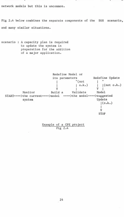
Fig 2.4 below combines the separate components of the SOS scenario,

and many similar situations.

scenario A capacity plan is required to update the system in preparation for the addition

of a major application.

Redefine Model or its

I

I

V

Monitor Build

parameters Redefine Update A(not

I

I

o.k.)

I

j(not o.k.)

I

V

I

a Validate Model START--->the current---->model

system

---)the model---->suggested Update

j(o.k.)

Example of a CPE project Fig 2.4

I

V

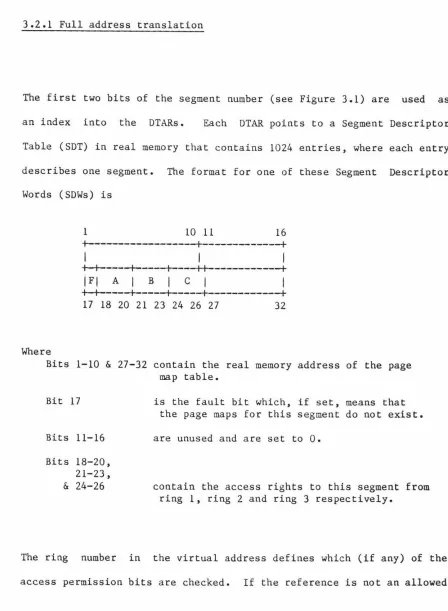
[image:24.551.77.499.90.826.2]

3 The principles of software monitoring

This section examines software monitors in more detail, particularly

o their structure,

o the indices that can be usefully measured (and how they are

measured), and

o the ways in which the measurements can be reported to the

performance analyst.

3.1 The structure of software monitors

As software monitors are used on many systems for different purposes no general structure covers all the cases, however Fig 3.1 shows the

basic components of most monitors. It is interesting to note that

+---+

1 Measurement

j--->

Immediate reporting

+---+

I

!(Record data) V

+---1 Recorded data

+---1

I

V

.--->

Summary reports

+---+

I

I

Report generator

1----1

+---+

\

'--->

Detailed reports

Structure of software monitors Fig 3.1

Some monitors (e.g., SUD for the IBM MVS operating system [FLETCH),

OPT/3000 [HP2) and Mesa Spy [McDa82)) report their measurements

interactively. These monitors have been designed to allow transient

problems to be corrected as they occur. For example using SUD may

show that some process has so much memory allocated to it that other processes are suffering. The amount of real memory allocated to it can then be reduced to free memory for other processes, and hopefully

this will improve the performance of the system as a whole.

If there is no need to obtain immediate results from a monitor, several advantages can be identified to saving the data as it is collected and producing reports at a later time. Some of these

o The monitor does less processing during the measuring period

and so there should be less distortion.

o Results can be studied at leisure rather than in real time.

o Different levels of report can be generated, such as:

- summary reports of the data, and

- detailed reports on

particular interest).

3.2 Performance indices

request (covering periods of

The following indices have been obtained by one or more of the

monitors described in [ROSE78], [BURR!], [BURR2], [McDA82], [KOLE71],

[SPERRl], [CALL75], [HPl] and [HP2]:

Number of users on the machine Mean session length

Standard deviation of session length Think time

Terminal response time Transactions per hour System availability

Data communications availability CPU utilisation

CPU states

CPU service time Length of CPU queue

Number and source of interrupts Memory utilisation

Memory contents (data, program, etc.) Memory distribution

Number of processes in memory Channel utilisation

Number of words transferred on each channel I/Os per second

Mean 1/0 stream length Overlay rates

Swapping rate

Device activity rates Device service times

In addition to these indices some software monitors also keep a trace

of various events, such as

I/Os

Page-outs

Process details

e.g. process identification device

record number.

e.g. time

process identification

page address (virtual or physical).

e.g. process identification start time

end time I/0 time used CPU time used.

3.3 Measuring disciplines

There are two common approaches to data collection by software

monitors. These are

o event trapping, and

o sampling.

A third method that is rarely used, but is sometimes mentioned in

discussions on software monitoring, is the

o backstop process.

This is a process with the lowest possible priority level whose only

task is to measure CPU time which would otherwise be idle. It is

worth noting that most machines allocate CPU time in quantum slices, and therefore this extra process could cause an additional overhead

during potentially profitable work time, as shown in Fig

3.2.

No other application ready for CPU so backstop quantum allocated

I

I

Application becomes runnable

End of backstop quantum, application is given the CPU

V V V

--->

_time

Backstop quantum Application quantum

1---11---

·

·

Wasted time

1---1

3.3.1 Event trapping

Often the index we wish to measure only changes when certain

operating system events occur. If we modify the code which produces

an event so that it records data on the event, then we have

implemented an event trap.

Unmodified code for event

I

I

I

I

I

_I

I /

V

i/

Code to record data about the event

I\

I

I

\

_I

I

' ,

I

I

V V

Event trappin~ Fig 3.3

Event traps require

o the data to be recorded at the time of the event;

o the code producing the event to be identified;

3.3.1.1 Collecting the data

Collecting the data may simply involve recording the fact that the

event has taken place (by incrementing a counter), or it may

involve retrieving data from memory or registers.

Depending on the nature of the event and the information required

about it, event trapping may be used to record data about every

event or, where a statistical measure is sufficient, the overhead

of the monitor may be reduced by only collecting data about a

fraction of the events.

The index being measured should not, in a statistical sense, be

dependent upon the occurrence of the event. For example,

attempting to measure the mean length of a queue by sampling its

length whenever an item is added to the queue will not produce an

accurate result. Rather the queue length should be sampled at

fixed time intervals.

3.3.1.2 Recording the data

The data may be recorded by one of three methods:

1) Adding to an accumulator location. For example, the total

active time of each disk channel may be obtained by a trap. Code

is added so that at the completion of a disk transfer a register,

the last item is read. This value can be added, by the trap code, to a location in memory, which will then be a running total of the amount of time the disk has been active. At some regular interval this location could be read and a derivation of the summation included in a report. This approach only applies to those cases where the data collected can be reduced to a simple summation, for example to, obtain a mean value.

2) The data collected may be written immediately to a secondary storage device and at some later time a report can be generated from the data. The cost of writing to a secondary device is normally quite high (in terms of the relative time taken) which makes this method unsuitable in many situations. If, for example, a trap that requested a disk I/0 was inserted into the process exchange mechanism, the frequency at which this would be executed would degrade the performance of the machine beyond acceptable limits.

3) In an attempt to reduce the overhead of recording the data on secondary media an intermediate buffer may be used. The data is written to a main memory buffer, and another process, which runs throughout the monitoring period, collects the data from this buffer and writes it to a secondary device (or produces a report from it).

some flexibility introduced as to the time of the write and this

may be scheduled to fit around the normal workload of the machine.

Care must be taken to ensure that the buffer does not overflow

causing some data to be lost.

These data recording techniques are also used by hardware monitors.

3.3.1.3 Problems with event trapping

While event trapping is the most powerful and accurate of the

software monitoring tools there are difficulties with its

implementation, some of which are considered below.

3.3.1.3.1 Access

Many of the resources required to implement an event trap are

difficult to obtain. In particular the source code of the

operating system is required. Generally manufacturers do not make

this available, but if they do they might not be willing to supply

the additional tools required to carry out the necessary

modification. Such tools might include a data dictionary,

external documentation, and compilers for modules written in

languages such as PLP (a PL/1 derivative used in Primos).

Even if all the source code and required tools are available,

Getting to understand the way a complex computer system works requires considerable time and effort, and may become so costly that it outweighs the advantages of monitoring the system. Also, altering and testing an operating system requires dedicated access to the system for relatively long periods of time.

3.3.1.3.2 Overheads

Accurately recording the extra overhead created by the insertion of code into an operating system is generally impossible. It can be estimated by using a benchmark on the two versions of the operating system, but this is subject to the availability of a good (honest) benchmark. Often the recording overhead is simply considered part of the operating system costs and is lost in that great debt.

3.3.1.3.3 Sensitivity

3.3.2 (Random) Sampling

The problems of event trapping may be avoided if a random sampling technique can be used. A monitor using random sampling may be implemented as a normal user process and so can avoid many of the difficulties associated with event trapping.

+---+

I

OPERATING SYSTEM

I

I

I

I

I

I

+----+

variable 1<----of interest

+----+

I

<

I

+---)---+

( USER PROCESSES

) (

Take Sample<--1

I

V

Record Sample

I

I

V Wait

I

I

'

+---+

Random sampling Fig 3.4

of achieving this is to sample at a regular time interval; however we will also discuss the following alternatives:

o Weighted sampling.

o Loosely coupled sampling.

3.3.2.1 Collecting the data

With random samples we do not have the choice of taking a sample every time the variable changes and thus cannot get a complete history of the index in question. We are unable, for example, to measure the time interval between a page being removed from main memory and it being recalled. To do that we would need data (the current time) to be collected at specified events (the page being rolled out and then being accessed again). We can however get a good measure of the mean value of an index, and the way it varies from this mean, provided sufficient samples are taken.

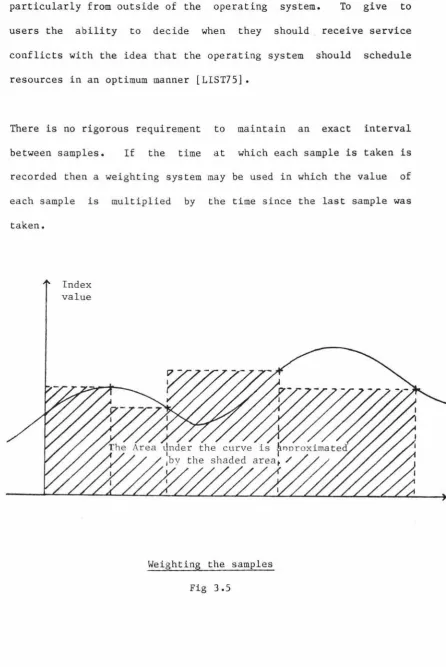
particularly from outside of the operating system. To give to users the ability to decide when they should receive service conflicts with the idea that the operating system should schedule resources in an optimum manner [LIST75].

There is no rigorous requirement to maintain an exact interval between samples. If the time at which each sample is taken is recorded then a weighting system may be used in which the value of each sample is multiplied by the time since the last sample was

taken.

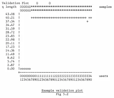
Index value

[image:37.550.67.514.76.744.2]

set up the semaphore

I

I

I

I

V <> 0 This means that ---)Test the semaphore---> we cannot keep up

counter with the sampling rate

I

so signal ERROR

I

V

Wait on the semaphore

I

I

V

Take the sample

I

I

,

<=====

The semaphore is notified by Primos

The sampling methodology

time

---11---11---11---11---11--->

_{A A A A A A}

I I

Semaphore signalled by the operating system.

Sample taken.

Example of sample timings

A loosely coupled sampling function Fig 3.6

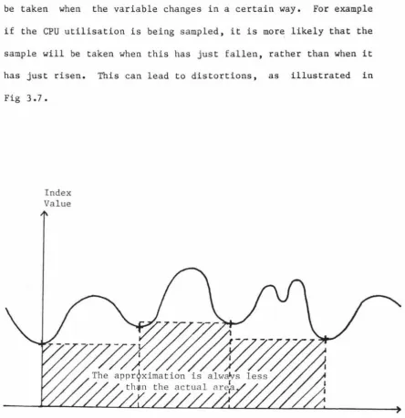
Both the non-regular sampling methodologies we have presented rely

on the underlying assumption that the variables we are sampling

be taken when the variable changes in a certain way. For example if the CPU utilisation is being sampled, it is more likely that the sample will be taken when this has just fallen, rather than when it has just risen. This can lead to distortions, as illustrated in

Fig 3.7.

Index

Value

Microscopic distortions Fig 3. 7

[image:40.552.76.520.72.530.2]

use these techniques, are that this is not the cause of errors that

are significant when compared with the accuracy of the monitor.

3.3.2.1.1 Collecting data by unit workloading

In chapter S we introduce a monitor that makes use of a variant of

the random sampling technique called unit workloading. This is

suggested, within this thesis, as an alternative approach to data

collection that avoids several of the problems of the usual

methods. As far as we can tell this technique has not been used

elsewhere.

With unit workloading the sample values are not a direct measure

of any resource in the system, but are the times taken to perform

some small operation. For example, a measure of how busy a disk drive is can be found from running a small benchmark arranged (as

in Fig 3.8) so that the main resource required during the timing

I

I

V Get a new

I

I

V Take the

I

I

V

time slice

time

\

I

I

I

I

Write a fixed

I

number of characters

to the disk

I •••

This code is loaded

I

I

V Take the

I

I

V Calculate the

I

V

time

I

I

into the same page to

I

avoid page faults

I

during the measurement

I

I

difference

A disk mini-benchmark Fig 3.8

3.3.2.1.1.1 Advantages of unit workloads

The advantages of this method of gathering data include the following:

o It allows any resource to which the programmer has access to be measured by random sampling.

the structure of the underlying system because they make

indirect measurements. Most of the code for such a

monitor could be used directly in the implementation a

similar monitor on another machine, that supported the

same programming language(s).

3.3.2.1.1.2 Disadvantage of unit workloads

The main disadvantage is the level of indirection introduced by

not measuring the index directly. This requires the monitor to

be calibrated and the results quoted as relative to this

calibration. The execution time for the benchmark when it is the

only user process on the system is a useful baseline for

calibration.

3.3.2.2 Recording the data

The same options are available for recording the data in random

sampling as in event trapping. However, there is not the same

emphasis on recording the data quickly as there was for the event

trapping mechanism, because, as a normal user, we are not likely to

alter any time critical system function, and also the overheads can

3.3.2.3 Advantages of random sampling

Apart from overcoming the specific disadvantages mentioned in the event trapping section, random

advantages:

sampling

o Distortions can be minimised.

o Installation is simpler.

3.3.2.3.1 Reducing distortion

has the following

Most preferable

I

~--->!

I

I

I

V

I

I

I

I

I

I

I

I

I

I

I

I

'

Prepare to sample

Wait

I

I

V

till next sample is due (system settles)

Take

I

I

V

the sample

I

I

,

Least preferable

I

.--->!

I

V

Prepare to sample

I

I

V

Take the sample

I

I

V

Wait till next sample is due

I

I

,

Reducing distortion Fig 3.9

If the operating system is not modified then there is no chance

that we will accidentally make it less efficient. Because the

operating system is a very active piece of software small errors

can have a large affect on system performance. A simple error

could, for example, invalidate the disk scheduling algorithm and

3.3.2.3.2 Simplicity of installation

The monitor is just another user program. It may be added to the system (or removed from it) without any disruption to other users. When it is not in use there is no residual overhead.

3.3.2.4 Problems with random sampling

The problems with random sampling are:

o Only those indices that can be treated statistically can be measured. We can measure queue lengths and device utilisations but cannot measure event counts or event type proportions.

o There is normally a high memory overhead in introducing a new process into the system.

3.4 Reporting the results of monitoring

The way the output of a monitor is presented can greatly affect its usefulness. If too much data is presented the user may be swamped with detail, but if too little is presented then important results could be hidden. Two approaches are often used to minimise these problems:

o multilevel reports.

o Data presentation techniques.

In section 3.1 we noted that if data reduction is left until after the measurement period, several passes over the recorded data can be made. Initially a summary report could be generated, and if there is a need for detailed reports then these could subsequently be produced

for the devices or time periods of interest.

The survey of monitoring projects mentioned in section 3.2 identified

a number of ways measurement data could be reported, namely:

o Quoting the indices (as a number) o Tables

o Histograms o Graphs

3.4.1 Quoting the indices

Quoting the value of the index is the simplest form of data presentation. For example

The paging rate= 12.3 pages/sec.

3.4.2 Tables

USERCODE

TSG

GAS

SPUR68PROD

ADG

LIT PUBS AVI

INVENTORY SPUR68DEV SECRETARY SHOOK SUPERVISOR

3.4.3 Histograms

B6800 SMFII ANALYSIS TASKIOTIME LSS 2000 SORTED BY ITEM 3 (ASCENDING)

MEAN(TASKPROCTIME) MIN(TASKELAPSEDTIME)

13 .23 0

401. 7 3 3

1.60 3

8.95 5

2.63 8

2.81 15

21.50 18

0.71 155

4.00 327

5.86 346

2.67 512

3.00 524

9.08 2515

A more visual, but generally less accurate, approach to presenting a

set of related indices is to use a histogram. The following diagram

B6800 SMFII ANALYSIS

TIME RANGE: 18:06:52 09/18/80 - 03:57:56 09/19/80

(*) RELATIVE HISTOGRAM OF AVAILMEM

21 -

l**********I

%

l**********I

% 24 -

l**********l**********I

21 -

l**********l**********l**********I

P 20

-**********l**********l**********l**********I

E

l**********l**********l**********l**********I

R

l**********l**********l**********l**********I

C

l**********l**********l**********l**********I

E

l**********l**********l**********l**********I

N

l**********l**********l**********l**********I

T 8

-**********l**********l**********l**********l**********I

l**********l**********l**********l**********l**********I

%

l**********l**********l**********l**********l**********I

%

l**********l**********l**********l**********l**********I

0

1---1---1---1---1---1

58.82 368.99 679.15 989.32 1299.48 1609.65 SCALE: X 100

<---

VALUES OF AVAILABLE MEMORY--->

3.4.4 Gantt profiles

Two variants of the Gantt Chart are discussed in CPE literature. We distinguish between them by the names Utilisation Profile [FERR78], and utilisation Time Profile.

CPU busy

Channel 1 busy

CPU and Channel 1 busy

so

SO%

30%

15%

Example utilisation profile Fig 3.10

- - --

-100%

I

I

I

I

I

I

I

I

A Utilisation Time Profile is a timing diagram showing the times the

resources were being used. The following is the time dependent

equivalent of Figure 3.10.

CPU busy

Channel 1 busy

CPU and Channel 1 busy

0

The monitoring interval in time units

S 10 15 20 25 30 35

Example utilisation time profile Fig 3 .ll

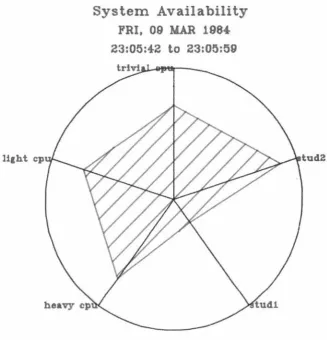
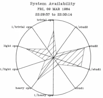
3.4.S Kiviat graphs

A Kiviat graph is a pictorial method of displaying more than two

system indices on a single diagram. The diagram is arranged around

a point, with an equally spaced radial axis for each index. The

index is plotted as a point on its axis and points on successive

axes are joined with line segments.

Variants exist on the basic chart, depending on the discipline (if

any) for choosing what index to display on each axis. The two major

variants are described by Ferrari [FERR83] as Noe's version (fig

3.12), where no discipline is used to choose the axes, and Kent's

version (fig 3.13), where successive axes plot positive then

negative indices. In the first case we use only positive indices

(ones which get bigger as performance improves), and the bigger the

area contained by the plot the better the system is performing; a

well balanced system will have a regular polygon (all angles the

same). With Kent's version the plot of a system which is performing

well will produce a star shape. A well balanced system will have

li1ht cp

System Availability

FRI, 09 MAR 1984

23:05:42

to

23:05:59

Example of Noe's version Kiviat graph

Fig 3.12

[image:53.553.129.456.164.503.2]

- -

-

- -

-

-

- -

- -

-

- - -

-System Availability

FRI, 09 MAR 198.f.

22:29:57

to

22:30:14-Example of Kent's version Kiviat graph

Fig 3 .13

tud2

[image:54.558.123.480.164.507.2]

4 Monitoring the Prime P75O

In chapter 3 we listed the following performance indices obtained by one or more of a number of software monitors reported in the literature:

Number of users on the machine Mean session length

Standard deviation of session length Think time

Terminal response time Transactions per hour System availability

Data communications availability CPU utilisation

CPU states

CPU service time Length of CPU queue

Number and source of interrupts Memory utilisation

Memory contents (data, program, etc.) Memory distribution

Number of processes in memory Channel utilisation

Channel transaction rates Channel service time Channel waiting time Channel queue length

Number of words transferred on each channel I/Os per second

Mean I/O stream length Overlay rates

Swapping rate

Device activity rates Device service times

and event traces of

I/Os Page-outs

In this chapter we address the feasibility of measuring these indices on the Prime P750.

The operating system for the Prime P750 is Primos. As we will be discussing measuring, interfacing and analysing Primos, an overview of the operating system and the related features of the P750 hardware is given in Appendix A.

4.1 Indices that could be measured

Primos lends itself to the measuring of several of the indices on the list.

4.1.1 Number of users

The number of users logged onto the system can be found by using an operating system routine provided for this purpose. USER$ gives a count of all users logged onto the system, including those from other machines and phantom users (a phantom is identical to a normal user except that input must be read from a file and not a terminal).

time.

4.1.2 Session length

If the external logon/logoff programs recorded the user number and

the time during logon and logoff, this data could later be analysed,

and the difference between logon and logoff time for each session

calculated and accumulated into a mean.

4.1.3 Think time

Ferrari [FERR83) defines the think time as" the time between

the end of a command's processing by the central subsystem and the

end of the inputting of the next command by the user."

A common Primos routine (ClIN) is used for all terminal input and

this routine could be patched to record data about the length of

time between the system requesting a command and the user typing one

in. This routine, like DISKIO, has a high usage and so the data

should be recorded carefully. Probably the most useful information

is the mean think time and this could be found using two accumulator

locations which held, respectively,

o the number of commands read;

o the total delay between requesting commands and their being

The mean think time for all terminal inputs since the system was

booted could be calculated at any time from these totals. The mean

think time over an interval could be calculated by taking the

difference between the two totals for the beginning and end of the

time period.

The think time as described above, assumes that the CPU time

required to accept the individual characters of a command is

negligible. A more detailed analysis could be done if two following

types of think time were identified:

o the time between the completion of one command and the user

entering the first character of the next command, and

o the time between successive characters in the command being

entered.

These could form part of the source data to a queueing network model

with two classes of job.

4.1.4 Terminal response time

There is no single definition of response time and with appropriate

patches a number of the possible response times could be measured.

measurements, consideration needs to be given to recording this data

without creating very much overhead, as the monitoring code will be

relativity heavily utilised. As with think times the mean would be

the most useful statistic.

4.1.S Transactions per hour

The precise nature of a transaction is also unclear and it would

need to be defined in Primos terms before it could be measured.

4.1.6 System availability

The down time for the system could be measured by several different

methods. For example, if the current date and time were

periodically written to the first record of a file, then the last

recorded time could be compared with the time when the system is

booted (after a crash) and the difference calculated. The accuracy

of this method would depend on the frequency at which the time was

recorded.

4.1.7 Data communications avail~bility

Primos can support the three types of network:

o Point to point, and

o Public data network,

and so the nature of a detailed report concerning data communications availability would depend on the configuration that existed use in the installation under consideration.

It should be possible to record the time for which a connection to each of the other machines in the network could be made. One way for a software monitor to do this would be to execute the Primos command 'status network' at a regular interval and record the results and the current time. This could be analysed later to produce a table giving the percentage of the measurement period that each remote system was available. The amount of quantisation error involved would depend on the sampling frequency.

4.1.8 CPU measures

Provision is made to record how much CPU time is used by each

processes. To do this the hardware regularly increments a register

in the processor's register file. This register is swapped, along

with the user accessible registers, by the process exchange

mechanism (process exchange is described more fully in Appendix A).

Primos accumulates this time into a total CPU time for each process,

consequently it is not too difficult to proportion the total CPU

time used between processes.

In particular the amount of time used by the backstop process can be

found. This is roughly equal to the amount of time the CPU would be

idle if the backstop did not exist. (It is only roughly correct as

the backstop does do some useful work (see Appendix A, section 5.3).

The length of the queues used for scheduling the CPU can be measured

by reading the count from the semaphore headers as discussed in section 4.1.8.1.

Other data about the CPU, such as the CPU states and CPU service

time, is not readily available to a software monitor.

4.1.8.l The length of the CPU queue

There are several lists on which processes that wish to use the CPU ·

are suspended; there is no single CPU queue. In the early stages the process waits on system semaphores known as wait-lists. Each

processes (see Appendix A, section 5.2), and this count could be

read and recorded by a software monitor. In the later stages the

process waits on the ready-list. No count of the waiting processes

is kept in the ready-list structure (Appendix A section 5.3.1), but

a software monitor could chain through, and count, the processes

waiting on each of the sub-lists.

4.1.9 Memory contents

It is not possible to determine the contents (data/ program/

linkage) of a segment from its virtual address, or from other data

available in the system, as the programmer may allocate segments

however he wishes. It is however possible to tell, from the segment

number, whether the segment is being used for the operating system,

other shared utilities (and on any one system the address number

will indicate the utility), or private user memory. This is because

under Primos segments l-1777(octal) are reserved for the operating

system, segments 2000-3777(octal) are reserved for shared programs

other than the operating system (the System Administrator defines

these and the addresses which they occupy), and segments

4000-7777(octal) form the user's private (non-shared) address space.

This division of the address space is discussed further in Appendix

A section 3.1.

A useful measure could be obtained by periodically working through

4.1.10 Channel measure

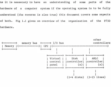
The exact nature of a channel on the P750 is clouded by the fact that all I/0 (including that know as Direct Memory Transfer (DMX)) passes through the central processor. This is implemented by way of a micro-code branch which transfers the data from the I/0 bus to the memory bus. The resources involved with disk I/0 transactions (most of which use one of the four types of direct memory transfer) are the I/0 bus, the cache, the memory bus, the disk controllers and the disks themselves (see Fig 4.1.)

+---t

memory bus

+---t

I/0 bus

I Memory!(---)! CPU!(--->

+---t

+---t

I

I

I

I

I

I

+---t +---t +---t

! Virtual I I Disk 1 AMLC I ! control ! !controller! !controller! ! panel 1 ! (s)! ! (s)l

+---t +---t +---t

I

I

(1-4 disks) (1-16 lines) Structure of P750 I/0 architecture

Fig 4.1