Is enough enough?
⋆What is sufficiency in
biometric data?
Galina V. Veres, Mark S.Nixon and John N. Carter
Department of Electronics and Computer Science University of Southampton, Southampton, SO17 1BJ
Abstract. Gait recognition has become a popular new biometric in the last decade. Good recognition results have been achieved using different gait techniques on several databases. However, not much attention has been paid to get major questions: how good are biometrics data; how many subjects are needed to cover diversity of population (hypothetical or actual) in gait and how many samples per subject will give good rep-resentation of similarities and differences in the gait of the same subject. In this paper we try to answer these questions from the point of view of statistical analysis not only for gait recognition but for other biometrics as well. Though we do not think that we have a whole answer, we content this is the start of the answer.
1
Introduction
Several biometrics databases were collected in the last decade and many good recognition results have been reported in the literature. However, not much was done to answer the questions will these results be valid for larger dataset? Some studies include a measure of recognition uncertainty, which is a guide to perfor-mance on a larger database and can serve to give confidence - the reliability of results. How can these results be used to make conclusions about some popula-tion? Is there enough data to get statistically significant results for chosen values of Type I and II error? How does one design a new dataset to get statistically significant results using available benchmark? In this paper we try to find some answers to these questions. Previously several works were published which con-cerned samples size [10, 9, 1, 5]. In this paper we use bounds on the minimum number of samples that guarantees that our future datasets will provide a good estimate of error rate using similar assumptions about distributions of error rates as reported in [5]. We estimate sample size, number of subjects and number of samples per subject assuming that the errors are independently distributed and the binomial law can be approximated by the Normal law. We consider whether some known databases have enough samples to make their results statistically significant. Finally, we looked at how the size of population determines the num-ber of subjects which required to obtain statistically significant results.
The paper is organised as follows. Section 2 presents problem formulation. Formulas for calculating number of samples, number of subjects and number
⋆
of samples per subject are given in Section 3. The design of future datasets is summarized in Section 4. Section 5 verifyes results for some available databases. How population size affects the required number of subjects is presented in Section 6. Finally Section 7 concludes the paper.
2
Problem formulation
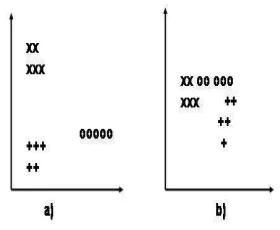
[image:2.595.250.390.359.474.2]In biometrics, measurements are abstracted from sensor data. In vision-based biometrics such as face, gait or palm-print recognition, measurements are de-rived from image data which, say, reflect the topology of target features. When multiple measurements are acquired and stored in a feature vector, each sub-ject can be represented in a mutidimensional space; a 2D measurement space is shown for convenience in Fig. 1. No assumptions have been made about distri-bution of measurements and graphs are presented for illustration purpose only. Graph a) shows a case when subjects are well separated and graph b) shows more realistic case when feature spaces for different subjects are interconnect. In this space there are a number of subjects for each of whom a number of
Fig. 1.Possible feature locations for three different subjects (X,+, O) in 2D case
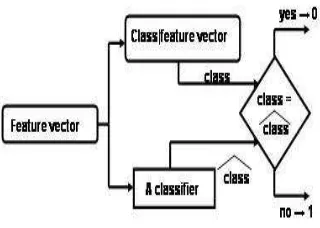
The number of subjects/ groups is clearly of interest since biometrics con-cerns identity, and identity is unique. Consider the introduction of one extra subject: if the new subject falls without the features already recorded then the recognition performance is unlikely to be affected. If on the other hand the ex-tra subject falls within the stored features, then recognition will be influenced by proximity to other subjects. For simplicity, we shall assume that subjects have the same number of samples per subject. The goal of a biometric system is to reduce recognition error by as much as possible for the sample population, whilst leading to a more general conclusion for a larger population. The errors in recognition (the misclassifications by the biometric system) can be represented by a function of the feature vectors obtained for each subject. The dependancy between biometric feature vectors and recognition errors is shown in Fig. 2 where the recognition errors are binary.
Fig. 2.Recognition process of gait data
LetXijfwill befth feature forjth repeated samples ofith subject withf =
1, . . . , Nf,Nf is a number of features,i= 1, . . . , Ns,Nsis a number of subjects
and j = 1, . . . , ng, ng is a number of samples per subject and n =Nsng is a
total number of samples per database. LetZijbe a binary variable and represent
the recognition results for jth sample obtained for ith subject, i.e. Zij = 1 if
there is a recognition error forjth sample ofith subject, andZij = 0 otherwise.
Zij are binomially distributed with probability pij of drawing 1 and (1−pij)
of drawing a 0, i.e. P r(Zij = 1|Xij.) = pij and Xij. = [Xij1Xij2. . . XijNf].
Then dependency between the probabilitypij of drawing 1 and feature vectors
Xij. can be expressed using the logit model. The logistic transformation of the
probability of drawing 1 is given by
logit(pij) = log(
pij
1−pij
). (1)
and obtained the loglit model
log( pij 1−pij
) =ηij =βi0+βi1Xij1+. . .+βiNfXijNf =
f=Nf
X
f=0
βifXijf, (2)
whereXij0= 1.
Solving for probabilitypij:
ˆ
pij =
exp(
f=Nf
P
f=0
βifXijf)
1 + exp(
f=Nf
P
f=0
βifXijf)
. (3)
For all possible values of X and β, the logistic transformation ensures that p
remains in the [0,1] interval.
The average error rate for an individuali will be calculated as
ˆ
pi=
1
ng ng
X
j=1
Zij, (4)
where i= 1, . . . , Ns and again the dependency between the average error rate
for individualiand variableZij can be written as a loglit model
log( pi 1−pi
) =
j=ng
X
j=0
βjZij and ˆpi=
exp(
j=ng
P
j=0
βjZij)
1 + exp(
j=ng
P
j=0
βjZij)
. (5)
These models can help to predict error rates due to new feature vectors. The average error rate for a whole data set is computed as
ˆ
p= 1
Ns Ns
X
i=1 ˆ
pi. (6)
Under assumption of identical and independently distributed data, recogni-tion errorsZij can be recognised as Bernoulli trials. Then the total number of
errorssinn=Ns∗ngtrials is distributed according to the binomial distribution:
ρn,p(s) =
µ
n s
ps(1−p)n−s, (7)
of meannp and variance np(1−p). And for a data set size of n samples, the estimate of error probability pis ˆp= s
n, where s is the number of errors. The
In gait recognition we are interested in confidence intervals. With a certain confidence (1−α), 0≤α≤1, we want the expected value of the error rate p
not to exceed a certain value
p <pˆ+ǫ(n, α), (8)
whereǫ(n, α) =βp, i.e.ǫ(n, α) is fixed to a given fraction β ofp. Then the null hypothesisH0is
H0:p−p < βp,ˆ (9)
and we want to test it with a confidence of being wrongα.
The random variable of which ˆp+ǫ(n, α) is a realisation is a guaranteed estimator of the mean. We are guaranteed, with riskαof being wrong, that the mean does not exceed ˆp+ǫ(n, α):
P rob(p≥pˆ+ǫ(n, α)) = X
np−s≥ǫn
ρn,p(s)≤α. (10)
Now we want to find a number of samples n, number of subjects Ns and a
number of samples per subjectng for which (10) holds.
3
Calculation of subjects number and number of samples
per subject for an infinite population
3.1 Number of samples in database
To estimate the total number of samples in the whole database, we will use the Chernoff bound [3], which asserts that with probability (1−α):
p−p <ˆ √−2 lnα
r
p
n, (11)
i.e.p−p < ǫˆ (n, α) with
ǫ(n, α) =√−2 lnα
r
p
n. (12)
A Chernoff bound is a lower bound and allows consideration of tails of distri-bution. The latter feature is quite important for binomial distribution, since the validity of the approximation of the binomial law by the Normal law in the tail of the distribution is questionable even for large values of the productnp.
Assuming that we can fixǫ(n, α) to a given fractionβ ofp
ǫ(n, α) =βp, (13)
we can assert, with riskαof being wrong that a number of samples
n=−2 lnα
is sufficient to guarantee that the expected value of error rate p is not worse than ˆp/(1−β). To use this formula,pneeds to be estimated from the results of previous benchmarks.
After recording a new database, it can be desirable to verify the statistical significance of the results. In this case the binomial law is approximated by the Normal law. We will not be able to say with certainty that we have enough samples to represent the population distributed by binomial law, but we will have the certain estimates for ideal case, i.e. normal distribution and it can serve as a guidance for estimation of the sample size.
The best recognizer will obtain an error rate ˆpand we would like to test the hypothesisH0:
p−p < βpˆ (15)
which for small values of p and under the assumption of normal distribution becomes:
p−p < zˆ α
r
p
n. (16)
Solving forp−pˆ, we obtain
p−p <ˆ z 2
α
2n(1 +
s
1 + 4npˆ
z2
α
) (17)
Therefore, if we pass the following test:
z2
α
2n(1 +
s
1 + 4npˆ
z2
α
)< βp (18)
we acceptH0 with riskαof being wrong. Otherwise, the number of examplesn is too small to guarantee a relative error bar ofβ.
Now we would like to find out the minimum number of subjects (groups) and number of samples per subject needed in the new database.
3.2 Number of subjects
We denote by Z.. = (1/Ns) Ns
P
i=1
Zi. the global mean over Ns subjects, where
Zi.= (1/ng) ng
P
j=1
Zij. The expected value ofZi. ispi and realizations of Zi. are
called ˆpi. The expected value ofZ.. ispand realizations of it is ˆp.
We call σ2
the “between-subject” variance and an estimate of this quantity is given by:
ˆ
σ2
≃
Ns
P
i=1
(ˆpi−pˆ)2
Ns
SinceZ..is the mean overNssubjects ofZi., its variance isσ2/Ns. Under the
assumption that the subject error rates are Normally distributed, the random variable
Z= p−Z..
σ/√Ns
(20)
obeys the standardized Normal law (with mean 0 and variance 1). Although the approximation of the binomial law by the Normal law is questionable in the tails of distribution it allows to get some estimates for the ideal case and these estimates will serve as a low bound for a real case.
With a riskαof being wrong, we have
p−p < zˆ α
σ
√
Ns
, (21)
where ˆp is a realization of Z.. and zα a threshold obtained from table of the
Normal distribution or conveniently approximated byzα≃
√
−lnα.
Then a guaranteed estimator of the average error rate per subject
p−p < ǫˆ (Ns, α) with ǫ(Ns, α) =zα
σ
√
Ns
. (22)
Remembering (13), we can assert, with riskαof being wrong, that a number of subjects
Ns= (
zασ
βp )
2
. (23)
is sufficient to guarantee that the expected value of the average error rate across subjects is not worse than ˆp/(1−β).
It is worth noticing thatσis a function of the number of examples per subject
ng. However, for large values ofng, it is largely independent ofng. Since
p
p/ng
is a lower bound ofσ, the hypothesis thatσis largely independent of ngwill be
verified whenng≫1/p.
3.3 Number of samples per subject
Now the problem of determining the number of samples per subject is addressed. We try to find a balance between “within-subject” and “between-subject” vari-ance. The following assumption is made that the empirical subject error rates are random variables Zi., normally distributed with mean pi and variance σ
2 , whereσ2
is “between-subject” variance, an estimate of which is given by (19). The number of examples per subjectngcan be expressed as a function of the
rationγof the “between-subject” varianceσ2
and the “within-subject” variance
w2
, which can be estimated from a benchmark data or some assumption can be made about it. Then
ˆ
γ= σ 2
w2. (24)
At the same time a total number of samplesn′=N
sng, then the number of
samples per subject can be calculated as
ng=
γn Ns
. (25)
4
Designing database sizes for future acquisition
We need to find out how many samples, subjects and samples per subject are needed for gait recognition to get statistically significant results. Gait recognition aims to discriminate individuals by the way they walk and has the advantage of being non-invasive, hard to conceal, being readily captured without a walker’s attention. It is less likely to be obscured than other biometric features. The large database (LDB) described in [8] is used as benchmark for calculating sample sizes for the new database. LDB consists of 115 subjects performing a normal walk and can help to determine which image information remains unchanged for a subject in normal conditions and which changes significantly from subject to subject, i.e. it represents subject-dependent covariates. We used our own database as benchmark for convience, since we know its structure and good recognition results were reported using this database [11]. It is assumed that a new database will be recorded in similar or near conditions to the recording of the benchmark and the quality of images in the new database will be not much worse than in the benchmark. These assumptions are quite realistic and ready to achieve. With confidence of 95% (α= 0.05), we want the expected value of error ratepto be not worse than 1.25 times the error rate of the best recognizer 1.25ˆp, i.e. β = 0.2,zα = 1.65. We will calculate samples size for the expected
values of error rates 0.01, 0.02 and 0.03, since many recognition papers reported the correct classification rate around or above 97%; and ˆp= 0.0153 which was estimated from LDB for the best classifier. Then the choice of samples size will be trade off between the expected error rate and time and recourses needed to record the new database. The following values were estimated using LDB: “between-subject” variance ˆσ2
= 0.0019 andγ≃3.
Then using formula (14), the number of samplesnin new database should be as in Table 1, i.e. to guarantee correct classification rate (CCR) of 99% we need almost 15000 samples in the database, practically 7500 samples are needed for CCR of 98% and lastly 5000 samples are needed for CCR of 97%. The numbers
Table 1.Number of samples, subjects and number of samples per subject needed p 0.01 0.02 0.03
n 14975 7490 5000 Ns 1294 324 144
ng 35 70 105
of subjects will be sufficient to guarantee that the expected error rate across all subjects is not worse than 1.25ˆp. Approximately 1300 subjects are needed to guarantee 99% CCR, 324 subject for 98% CCR and 144 subjects for 97% CCR. Since a number of subjects was obtained by approximation of the binomial law, it is better to take more subjects than the numbers reported if resourses and time are available for collecting bigger data sets. Finally, using formula (25) and results presented in Table 1 so far, we can calculate the number of samples per subject ng. The results are presented in Table 1. The number of samples
needed per subject is 35, 70 and 105 for 99%, 98% and 97% CCRs recpectively. When collecting 70 or 105 samples per subject, extra attention should be paid to the design of the experiment. Since walking for too long (around one hour for 70 samples) will make a person tired and the tiredness will affect their gait. Therefore it is advisable to divide recording to several slots and record the person during a couple of days. As it was reported previously gait is not affected by time when only days pass between recording sections [13].
5
Verifying the statistical significance of the results for
available databases
Several databases were recorded recently describing different biometrics such as gait, face, iris, finger print. We would like to look at some of the them from the point of the view of statistical significants of the results using formula (18). The databases considered are LDB describing gait from the University of Southampton mentioned above [12], CASIA iris image database [4, 2], FERET database of facial images [6], subset of BEN database of fingerprint images [14] and FRVT2002 database of faces [7]. CCRs reported for these databases and a number of samples used to obtain these CCRs are presented in Table 2. All these
Table 2.Characteristics of databases database LDB BEN FRVT2002 FERET CASIA
ˆ
p 0.0153 0.0103 0.27 0.03 0.0086 n 2161 12000 121589 2392 756
databases have a good number of samples collected in the similar conditions and CCRs around or above 97% were reported for all of them except FRVT2002, where CCR is 73%. We included FRVT2002 in our investigation since it has the highest number of samplesn= 121589. It would be interesting to see the results of applying formula (18) to such a big dataset.
Using the data from Table 2 the left-hand side of the formula (18) is cal-culated for each dataset with α= 0.05 and results are presented Table 3. For
β= 0.2 the right-hand side of the formula (18) gives 0.002, 0.004 and 0.006 for
Table 3.Verification of the statistical significance of the results LDB BEN FRVT2002 FERET CASIA
0.0051 0.0016 0.0025 0.0064 0.0076
database has enough samples for all expected values of the error rates to guar-antee a relative error bar ofβ. FERET and CASIA do not have enough samples for any chosen expected values of the error rates to guarantee a relative error bar ofβ. LDB and FRVT2002 have enough samples for some expected values of the error rate. All this means that either the number of samples in data bases has to be increased or if it is not possible the relative error bar ofβ should be increase if it is possible for a given applications.
6
Database size for a population of finite size
The number of subjects Ns obtained in Table 1 was calculated without
tak-ing into consideration the size of the population. When the population is large enough in comparison to the sample size or it is desirable later to extend analysis of data for larger population, then the number of subjects in Table 1 is valid. However, when population is comparibale in size with the sample size, the finite population correction factor is needed, i.e. the final number of subjectsnf will
be
nf =
Ns
1 +Ns
N
, (26)
whereN is a population size, Ns is a sample size. These statements are made
under assumption that the population is sampled uniformly. When it is not possible to sample uniformly from the population bigger sample sizes will be meeded.
Biometrics can be used both on a large population and on a relatively small one. For instance, gait recognition can be used to make identification and sta-tistical conclusions for population of Britain (58 million people) or to gain a security access to the firm of 10000 people. The question arises how the size of the population will affect the number of subjects needed for investigation? To get some approximate knowledge about final size, we look at the concrete example from Table 1, when number of subjects Ns = 324 for p = 0.02. The
dependency between size of populationN and final number of subject nf was
calculated, whereN will change from 500 to 15 million people by 100 people. The calculations showed that after some size of population the number of sub-jects needed to characterise this population stays practically the same. In this case, from size of populationN equals around 10.5 million people, the corrected number of subjects stays at the same level of 323.9 subjects, thus nf = 324,
and we got the final number of subjects 323.007 or nf = 324 for a population
size from 104400. This means that if we are dealing with the population size of
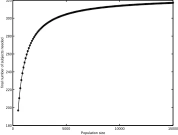
significant conclusions about this population and the finite population correction factor does not affect the results. So far we looked at what happens when the population is quite large. However, it is interesting how the number of subjects needed will change when the size of population is comparable to the sample size (here number of subjects). Fig. 3 shows a dependency between population size and the final number of subjects needed when the former is comparable in size with the later, i.e. in this case N = 15000 or below. In this case the finite
0 5000 10000 15000
180 200 220 240 260 280 300 320
Population size
[image:11.595.198.376.216.351.2]final number of subjects needed
Fig. 3.Dependency between population size and the number of subjects for smaller populations
population correction factor helps to reduce the small size noticeably for the population of 3000 people or below. After that the growth in the sample size is very slow and increase is from 293 subjects for the population of 3000 people to 317 subjects for the population of 15000 people. All these conclusions are valid when the population was uniformly sampled.
7
Conclusions
Acknowledgment
We gratefully acknowledge partial support by the Defence Technology Centre 8−10 supported by General Dynamics.
References
1. J.F. Bromahgin Sample Size Determination for Interval Estimation of Multinomial Probabilities The American Statistician, vol. 47, 203-206, 1993
2. CASIA iris database. Institute of Automation, Chinese Acadamy of Sci-ences.http://www.sinobiometrics.com/casiairis.htm.
3. H. Chernoff A Measure of Asymptotic Efficiency for Tests of a Hypothesis Based on the Sums of Observations Annals of Mathematical Statistics, vol. 23, 493-509, 1952
4. C. T. Chu and C. Chen High Performance of Iris Recognition Based on LDA and LPCC Proc. 17th IEEE International Conf. on Tools with Artificial Intelligence, Hong Kong, 2005
5. I. Guyon, J. Makhoul, R. Schwartz and V. Vapkin What Size Test Set Gives Good Error Rates Estimates? IEEE Trans. Pattern Analysis and Machine Intelligence, vol. 20 (1), 52-64, 1998
6. P.J. Phillips, H. Moon, S.A. Rizvi and P.J. Rauss The FERET Evaluation Method-ology for Face-Recognition Algorithms IEEE Trans. Pattern Analysis and Machine Intelligence, vol. 22 (10), 1090-1104, 2000
7. P.J. Phillips, P. Grother, R. Micheals, D.M. Blackburn, E. Tabassi and M. Bone Face Recognition Vendor Test 2002: Overview and Summary ftp://sequoyah.nist.gov/pub/nist internal reports/ir 6965/FRVT 2002 Overview and Summary.pdf, March 2003
8. J. D. Shutler, M. G. Grant, M. S. Nixon, and J. N. Carter On a Large Sequence-Based Human Gait DatabaseProc. 4th International Conf. on Recent Advances in Soft Computing, Nottingham (UK), 2002
9. S.K. Thompson Sample Size for Estimating Multinomial ProportionsThe American Statistician, vol. 41, 42-46, 1987
10. R.D. Tortora A Note on Sample Size Estimation for Multinomial PopulationsThe American Statistician, vol. 32, 100-102, 1978
11. G.V. Veres, L. Gordon, J.N. Carter and M.S. Nixon What image information is important in silhouette-based gait recognition? Proceedings of IEEE Computer So-ciety Conference on Computer Vision and Pattern Recognition, Washington, D.C., USA,II: 776-782 2004.
12. G.V. Veres, M.S. Nixon and J.N. Carter. Model-based approaches for predicting gait changes over time Proc. of International Workshop on Pattern Recognition, Beijing (China), 2005.
13. G.V. Veres, M.S. Nixon and J.N. Carter Modelling the time-variant covariates for gait recognition accepted to5th International conference on Audio- and Video-Based Viometric Person Authentication, New York, USA, 2005.
14. C. Wilson, R.A. Korves, B. Ulery. M. Zoepfl, M. Bone, P. Grother, R. Micheals, S. Otto and C. Watson Fingerprint Vendor Technology Evaluation 2003: Summary of Results and Analysis Report NISTIR 7123, June 2004, http://fpvte.nist.gov/report/ir 7123 analysis.pdf