Sparse support vector regression based on orthogonal forward selection for the generalised kernel model

author’s benefit and for the benefit of the author’s institution, for

non-commercial research and educational use including without

limitation use in instruction at your institution, sending it to specific

colleagues that you know, and providing a copy to your institution’s

administrator.

All other uses, reproduction and distribution, including without

limitation commercial reprints, selling or licensing copies or access,

or posting on open internet sites, your personal or institution’s

website or repository, are prohibited. For exceptions, permission

may be sought for such use through Elsevier’s permissions site at:

Author's personal copy

Sparse support vector regression based on orthogonal forward

selection for the generalised kernel model

X.X. Wang

, S. Chen

, D. Lowe

, C.J. Harris

School of Electronics and Computer Science, University of Southampton, Southampton SO17 1BJ, UK Received 4 February 2005; received in revised form 9 December 2005; accepted 17 December 2005

Communicated by J. Zhang Available online 18 May 2006

Abstract

This paper considers sparse regression modelling using a generalised kernel model in which each kernel regressor has its individually tuned centre vector and diagonal covariance matrix. An orthogonal least squares forward selection procedure is employed to select the regressors one by one, so as to determine the model structure. After the regressor selection, the corresponding model weight parameters are calculated from the Lagrange dual problem of the original regression problem with the regularised-insensitive loss function. Unlike the support vector regression, this stage of the procedure involves neither reproducing kernel Hilbert space nor Mercer decomposition concepts. As the regressors used are not restricted to be positioned at training input points and each regressor has its own diagonal covariance matrix, sparser representation can be obtained. Experiments involving one simulated example and three real data sets are used to demonstrate the effectiveness of the proposed novel regression modelling approach.

r2006 Elsevier B.V. All rights reserved.

Keywords:Generalised kernel model; Orthogonal least squares forward selection; Regression; Sparse modelling; Support vector machine

1. Introduction

Objective of modelling from data is not that a model should fit well to the training data. Rather, the goodness of a model is characterised by its generalisation capability, and the model should be easy to interpret and to extract knowledge from. All these vital properties depend on crucially the ability of a modelling process to obtain appropriately sparse representations. Forward selection using the orthogonal least squares (OLS) algorithm

[7–10,13] is a simple and efficient method that is capable of producing parsimonious linear-in-the-weights nonlinear models with excellent generalisation performance. Alter-natively, the state-of-the-art sparse kernel modelling techniques, such as the support vector machine (SVM)

[31,18,26–29,14,6,15], have become popular in data

model-ling applications. Originated from maximum margin linear classification, one of the main features of the SVM is to use hyperplane. Specifically, the training data are mapped to a high dimensional space where they can be approximated by a hyperplane. In classification, this hyperplane is adjusted to obtain the maximum classification margin. In regression, the gradient of this hyperplane is kept as small as possible. More precisely, in a SVM regression problem, the parameter of the hyperplane is obtained by minimising the cost consisting of the linear-insensitive loss function and the squared gradient of the hyperplane[18].

With the aid of the reproducing kernel Hilbert space through Mercer theorem [2], Mercer kernel can be used, and the required mapping from the input space to the high dimensional space is given implicitly by this kernel function. A common feature of the SVM regression modelling techniques as well as the OLS kernel modelling methods [7–10,13] is that the kernel centres are placed at the training input data and a fixed common kernel variance is used for all the regressor kernels. The value of this common kernel variance obviously has a critical influence

www.elsevier.com/locate/neucom

0925-2312/$ - see front matterr2006 Elsevier B.V. All rights reserved. doi:10.1016/j.neucom.2005.12.129

_{Corresponding author.}

Author's personal copy

resulting model, and it has to be determined via cross validation. If the positions of kernel regressors are more flexible and different kernel regressors can have their own diagonal covariance matrices, a better system model can be established. However, putting kernel function at a position not occupied by a train data point or giving different kernel regressors at different positions different covariance matrices are not allowed for the SVM methods that use Mercer theorem. Also this ‘‘generalised’’ kernel model will change the ‘‘linear’’ learning problem associated with the SVM-type models to a nonlinear one.

Unlike the SVM formulation, the method proposed in this paper minimises the cost consisting of the linear -insensitive loss function and the squared weights of the regressors. This formulation allows the use of non-Mercer kernels. Specifically, the ‘‘generalised’’ kernel function is used in which each kernel regressor has its tunable centre vector and diagonal covariance matrix. To arrive at a sparse representation, the OLS forward selection procedure is adopted to select regressors one by one by incrementally minimising the training mean square error (MSE). Unlike the standard OLS algorithm [7], however, at each stage of selection the optimisation is with respect to the kernel centre vector and diagonal covariance matrix, and the determina-tion of these kernel parameters is performed using a guided random search algorithm called the repeated weighted boosting search (RWBS) algorithm[12], which has its root from boosting optimisation [30,16,5,25]. Thus, regression modelling is carried out by a ‘‘kernel hunting’’. The ‘‘support vectors’’ are selected by the OLS criterion and, unlike the SVM, the number of regressors is not controlled by the value of the -insensitive loss function. After the selection of a parsimonious model representation, the kernel weights are then calculated from the Lagrange dual of the original minimisation problem. This proposed generalised kernel regression modelling approach has the potential of improving modelling capacity and producing sparser final models, compared with the standard SVM algorithm. The advantages of the proposed method are illustrated using a simulated example and three real-data sets.

The remaining of the paper is organised as follows. Section 2 reviews the standard kernel regression modelling, which positions the kernel centres at the training input data points and adopts a single common variance for every kernel regressors. The classical SVM formulation is first summarised. An alternative Lagrange dual problem of the general SVM problem is then considered, which does not restrict to the use of Mercer kernels. This method will be referred to as the extended SVM (ESVM). Unlike the standard SVM method, the solution obtained by the ESVM is not sparse. To derive a sparse representation, the standard OLS algorithm [7] is used to select a parsimonious model, and this is followed by solving the corresponding sparse ESVM problem to yield the model weight parameters. This method will be referred to as the sparse extended SVM (SESVM). The main contribution of

this paper is presented in Section 3, where the generalised kernel regression modelling is considered. A new OLS forward selection procedure is proposed, which uses the RWBS algorithm [12] to determine the kernel centres and diagonal covariance matrices. This guarantees a sparse representation. Again, the kernel weights are solved from a similar ESVM problem after obtaining a sparse representa-tion. This proposed new method will be called the generalised sparse extended SVM (GSESVM) for the purpose of comparison with the methods of Section 2. Section 4 provides the results of our modelling experi-ments, while Section 5 summarises our conclusions.

2. Standard kernel regression modelling

The task of kernel regression modelling is to construct a kernel model from the given training data set fxi;yigNi¼1,

wherexiis theith training input vector of dimensionm,yi

is the desired output for the inputxi andNthe number of

training data. The SVM method solves this problem by using the following strategy.

2.1. Support vector machine regression problem

The minimisation problem of the SVM method using the linear-insensitive loss function[18]can be stated as below:

minJðw;n;nÞ ¼min 1 2w¯

T_{w¯ þC} X N

i¼1

x_i þX

N

i¼1 xi

!

( )

,

(1)

subject to

y_iw¯T_uðx

iÞ bpþxi; 1pipN; ¯

wTuðxiÞ þbyipþxi; 1pipN;

x_iX0; 1pipN;

xiX0; 1pipN;

8 > > > > < > > > > :

(2)

where uðxÞ is the selected mapping from the input space to the high-dimensional space, y¼w¯T_{uðxÞ þb is the}

linear regression function (hyperplane) in the high-dimen-sional space withw¯ as its gradient,Cis a pre-specified value that defines regularisation, n¼ ½x1 x2 xNT and n ¼ ½x₁ x₂ x_NT are stack variables representing upper and lower constraints on the system outputs, and is a given value that defines the-insensitive loss function.

Let us define the Mercer kernel

kðxi;xjÞ ¼ huðxiÞ;uðxjÞi (3)

with h;i denoting the inner product in the high-dimensional space. It is well known that the dual problem of Eqs. (1) and (2) is:

maxL¯ða;aÞ ¼ max X

N

i¼1 ða

i þaiÞ þ

XN

i¼1 y_iða

i aiÞ

(

1

2

XN

i¼1

XN

j¼1 ða

i aiÞðaj ajÞkðxi;xjÞ

)

Author's personal copy

PN i¼1ða

i aiÞ ¼0;

0pa

ipC; 1pipN;

0paipC; 1pipN: 8

> < >

: (5)

After obtaining the Lagrange multipliers, a¼ ½a1a2 aNT and a¼ ½a1 a2 aN

T_{, and the bias term b, the}

regression model is given by

^

yðxÞ ¼X N

i¼1 ða

i aiÞkðxi;xÞ þb. (6)

It is well known that the use of the-insensitive cost function leads to a more robust parameter estimate, compared with the conventional least squares cost function. The choice of the -insensitive loss function is also attractive because many of the ‘‘weights’’a

i aibecome zero, leading

to a sparse solution in (6). One of the most common choices of kernel function is the Gaussian function of the form:

kðxi;xÞ ¼exp

kxxik2

2s2

. (7)

The common kernel variance s2 _{is not provided by the}

algorithm and has to be determined by other means, such as via cross validation.

2.2. Dual of the minimisation problem withe-insensitive loss function and squared regressor weights

Consider the modelling of the training data setfxi;yigNi¼1

with the regression model

^

yðxÞ ¼X N

i¼1

wihiðxÞ þb, (8)

wherewiis theith model weight, andhiðxÞis theith kernel regressor centred at the training inputxi. By adopting the

combined cost function of the -insensitive loss function and the squared regressor weights, the following minimisa-tion problem can be established:

minJðw;n;nÞ ¼min 1 2w

T_wþC X N

i¼1

x_i þX

N

i¼1 xi ! ( ) , (9) subject to

y_iPN_j¼1wjhjðxiÞ bpþxi; 1pipN;

PN

j¼1wjhjðxiÞ þbyipþxi; 1pipN; x

iX0; 1pipN;

xiX0; 1pipN:

8 > > > > < > > > > : (10)

Although the optimisation problem (9) and (10) appears to have the same form as that of (1) and (2), these two problems are different. Let us definew¼ ½w1 w2 wNT and

hðxiÞ ¼ ½h1ðxiÞh2ðxiÞ hNðxiÞT. (11)

The Lagrangian of the minimisation problem (9) and (10) can be written as

Lðw;n;n;a;a;c;cÞ

¼1

2w

T_wþCX N

i¼1

ðx_i þxiÞ

XN

i¼1 ðg

ix i þgixiÞ

X

N

i¼1

aiðy_iwThðxiÞ bþþxiÞ

X

N

i¼1 a

iðw T_hðx

iÞ þbyiþþxiÞ, ð12Þ

where a¼ ½a1 a2 aNT, a _{¼ ½a}

1 a2 aNT, c¼ ½g1

g₂ g_NT and c_{¼ ½g}

1 g2 gN

T _{are the Lagrange}

multipliers. From the Kuhn–Tucker conditions, we have

qL

qw¼w

XN

i¼1

ða_i aiÞhðxiÞ ¼0, (13)

qL

qn¼ ½C C C

T

ac¼0, (14)

qL

qn ¼ ½C C C

T

ac¼0, (15)

qL qb ¼

XN

i¼1 ða

i aiÞ ¼0. (16)

Substituting the Kuhn–Tucker conditions into Lagrangian (12) leads to the dual problem of the primal problem (9) and (10):

maxL¯ða;aÞ ¼ max X

N

i¼1

ða_i þaiÞ þX N

i¼1

y_iða_i aiÞ

(

1

2

XN

i¼1

XN

j¼1

ða_i aiÞða_j ajÞhTðxiÞhðxjÞ

)

,

ð17Þ

subject to

PN i¼1ða

i aiÞ ¼0;

0pa

ipC; 1pipN;

0paipC; 1pipN: 8

> < >

: (18)

After obtaining a _{and a, we can calculate the model} weights from (13) as

w¼X

N

i¼1 ða

i aiÞhðxiÞ. (19)

The key difference between the minimisation problem (9) and (10) and the SVM one given in (1) and (2) is that here regularisation directly controls the kernel weights, but not the gradient of the unseen hyperplane as is in the case of (1) and (2). Thus, this approach does not impose any restriction on the kernel function used. We refer to this approach as the ESVM method to contrast with the SVM method discussed in Section 2.1.

Author's personal copy

2.3. Construction of sparse ESVM models

One drawback of the aforementioned ESVM method is that solution (19) is generally non-sparse. To obtain a sparse model, we propose first to use the OLS algorithm [7] to select a parsimonious subset model from the full regression model (8). Without the loss of generality, we will assume the bias term b¼0 in model (8). In fact, this bias term can be regarded as a constant regressor. The regression model (8) over the training set can be expressed as

y¼Hwþe, (20)

where y¼ ½y₁ y₂ y_NT, e¼ ½e1 e2 eNT with ei¼ y_iwT_hðx

iÞ denoting the modelling error at the input xi,

and

H¼ ½h1 h2 hN (21)

is the regression matrix with the regressor columns or model bases defined by

hi¼ ½hiðx1Þhiðx2Þ hiðxNÞT; 1pipN. (22)

Let an orthogonal decomposition of Hbe

H¼PD, (23)

where P¼ ½p₁ p₂ p_Nwith orthogonal columns satisfy-ing pT_ip_j¼0 ifiaj, and

D¼

1 d1;2 d1;N

0 1 .. . ... ..

. . . .

. . .

dN1;N

0 0 1

2 6 6 6 6 6 4

3 7 7 7 7 7 5

. (24)

The regression model (20) can alternatively be expressed as

y¼PDwþe¼Phþe, (25)

where the orthogonal model weight vector h satisfies the triangular system h¼Dw.

The sum of squared errors for this N-term regression model can be expressed as[7]

JN ¼eTe¼yTy

XN

i¼1 ðyTp_iÞ2

pT_ip_i . (26)

Define the error reduction due to the jth termp_j as

ERj¼ ðyTp_jÞ2

pT jpj

. (27)

Based on this error reduction criterion, a subset model can be obtained in a forward selection procedure[7]. At thelth selection stage, a model term is selected from the remaining candidatesp_j,lpjpN, as thelth model term in the subset model, if it maximises the error reduction criterion ERj.

The details of the selection algorithm are readily available in [7–10,13] and is not repeated here. The selection is

terminated at theNsstage if the MSE

1

NJNspz, (28)

where the small positive tolerance value z controls the sparsity level of the selected subset model. This produces a parsimonious model containing Ns terms. Appropriate

value for z is problem dependent and may be learnt via cross validation. Alternatively, the Akaike information criterion [1,23] can be adopted to terminate the subset model selection procedure. Moreover, the optimal experi-mental design criteria can be combined with the least squares cost (26) to automatically terminate the selection with an appropriateNs-term subset model without the need for the user to specify a tolerance valuez[9,19,20]. It should also be pointed out that regularisation can naturally be incorporated into this OLS forward selection procedure[9]. As is in the standard kernel regression modelling, each kernel regressor is positioned at a training input data point and a single common kernel variance s2 is used for every regressors. Using the OLS forward selection procedure described above, we first obtain a sparse representation containing Ns kernel regressors. The corresponding

kernel weights are then calculated using the ESVM method of Section 2.2. We will referred to this approach of constructing sparse kernel models as the SESVM method.

3. Generalised kernel regression modelling

In Section 2.2, the deduction of the dual problem does not assume the concept of reproducing kernel Hilbert space and Mercer theorem. Therefore, we are not restricted to Mercer kernels. For example, we will allow a kernel function to take position other than the training input data points and to have an individually tunable diagonal covariance matrix. This leads to the generalised kernel regression modelling, in which the regressors take the form:

hjðxÞ ¼g

ffiffiffiffiffiffiffiffiffiffiffiffiffiffiffiffiffiffiffiffiffiffiffiffiffiffiffiffiffiffiffiffiffiffiffiffiffiffiffiffiffiffi

ðxl_jÞTR_j1ðxl_jÞ

q

, (29)

where 1pjpM, l_j is the mean vector of the jth kernel, Rj¼diagfs2j;1;sj2;2;. . .;s2j;mgits diagonal covariance matrix, M is the number of regressors in the model, and gðÞ a chosen kernel function.

3.1. Construction of sparse generalised kernel models

We propose a construction procedure for obtaining sparse generalised kernel models by adopting an orthogo-nal forward selection to append the regressors one by one. At the lth stage of model construction, the lth kernel regressor is determined by maximising the following error

Author's personal copy

ERlðll;RlÞ ¼ ðyTp_lÞ2

pT lpl

, (30)

where p_l is obtained by an orthogonal transformation of thelth model column hl ¼ ½hlðx1Þhlðx2Þ hlðxNÞT via

p_l¼hl

Xl1

j¼1

dj;lpj (31)

andp_j, 1pjpl1, are the orthogonalised model columns already selected. All the discussions in Section 2.3 regarding the termination of selection apply here. For example, the model appending process can be terminated when the MSE

1

NJMs¼

1

Ny T_y 1

N

XMs

l¼1

ERlðll;RlÞpz (32)

yielding an Ms-term generalised kernel model. The corre-sponding kernel weights can readily be calculated using the ESVM method of Section 2.2. For a comparison purpose, we will call this construction approach the GSESVM method.

3.2. Determination of the generalised kernel parameters

It can be seen that at each regression stage, the task is to determine the generalised kernel parameters u so as to minimise the cost function

fðuÞ ¼ 1 ERlðuÞ

, (33)

where the parameter vectorucontains the regressor mean vector ll and diagonal covariance matrix Rl. This

optimisation task may be carried out with a gradient based optimisation method. A gradient method however depends on the initial condition and may be trapped at the local minima. Alternatively, the standard global optimisation methods, such as the genetic algorithm[17,24]and adaptive simulated annealing [22,11], can be used. We have developed a simple and effective guided global search method called the RWBS algorithm[12], which is adopted to perform this optimisation task. The algorithm for determining the generalised kernel parameters at each incremental model stage is summarised as follows.

Repeated weighted boosting search: Specify the following algorithmic parameters: PS—population size, NG —num-ber of generations in the repeated search, andzI—accuracy

for terminating the weighted boosting search.

Outer loop: generationsFork¼1:NG

Outer loop initialisation: Initialise the population by setting uð₁kÞ¼uð_bestk1Þ and randomly generating rest of the population members uð_ikÞ, 2pipPS, where uðbestk1Þ denotes

the solution found in the previous generation. Ifk¼1,uð₁kÞ

is also randomly chosen

Weighted boosting search initialisation: Assign the initial distribution weightings dið0Þ ¼1=PS, 1pipPS, for the

population

(1) For 1pipPS, generateh_l½ifromuð_ikÞ, the candidates for thelth regressor, and orthogonalise them:

d½_ji_;l ¼p T jh

½i

l

pT_jp_j ; 1pjol, (34)

p½_li¼h½_liX l1

j¼1

d½_ji_;lp_j. (35)

(2) For 1pipPS, calculate the loss of each population

member

S½_li¼fðuð_ikÞÞ ¼ðp

½i

l Þ T_p½i

l ðyT_p½i

l Þ

2. (36)

Inner loop: weighted boosting search Set t¼0; For

tþ ¼1

Step 1:Boosting

(1) Find

u_bestðkÞ ¼arg minfS_l½i;1pipPSg,

u_worstðkÞ ¼arg maxfS_l½i;1pipPSg.

(2) Normalise the loss function values

¯

S½_li¼ S

½i

l

PPS j¼1S

½j

l

; 1pipPS.

(3) Compute a weighting factorb_t according to

Z_t ¼X

PS

i¼1

diðt1ÞS¯_l½i; b_t ¼ Zt 1Z_t.

(4) Update the distribution weightings for 1pipPS

diðtÞ ¼ diðt1Þb ¯ S½li

t forbtp1; diðt1Þb

1S¯½li

t forbt41;

8 < :

and normalise them

diðtÞ ¼_PPSdiðtÞ j¼1djðtÞ

; 1pipPS.

Step2:Parameter updating

(1) Construct theðPSþ1Þth point using the formula

uPSþ1¼

XPS

i¼1

diðtÞuðikÞ.

(2) Construct theðPSþ2Þth point using the formula

uPSþ2¼uðbestkÞ þ ðu

ðkÞ

bestuPSþ1Þ. X.X. Wang et al. / Neurocomputing 70 (2006) 462–474

Author's personal copy

orthogonalise these two candidate model columns (as in (34) and (35)), and compute their loss function values (as in (36))

(4) Choose a better point (smaller loss function value) from

uPSþ1 anduPSþ2 to replaceuðworstkÞ

IfkuPSþ1uPSþ2kozI, existinner loop

End of inner loop

The solution found isuð_bestkÞ End of outer loop

This yields the solutionu¼uð_bestNGÞas the parameter vector (mean vector and diagonal covariance matrix) of the lth regressor, as well as the corresponding orthogonal model columnp_l.

The motivation and analysis of the RWBS algorithm as a general global optimiser are detailed in [12]. The appropriate values for the algorithmic parameters, PS, NG andzI, depends on the dimension of uand how hard

the objective function to be optimised. Generally, these algorithmic parameters have to be found empirically. In the inner loop optimisation, there is no need for every members of the population to converge to a (local) minimum, and it is sufficient to locate where the minimum lies. Thus, the accuracy for stopping the weighted boosting search,zI, can be set to a relatively large value. This makes

the search efficient, achieving convergence with a small number of the cost function evaluations. As an alternative to choose zI, one can simply set a maximum number of

iterationsMIfor the inner-loop optimisation. The popula-tion sizePS and the number of generationsNGshould be

set to sufficiently large values so that the parameter space will be sampled sufficiently. The optimisation experiments reported in[12] suggested that the algorithmic parameters of the RWBS algorithm are not difficult to set.

It should be emphasised that PS,NGandzI(orMI) are

not the learning hyperparameters of the GSESVM algo-rithm. Rather they are the optimisation algorithmic parameters. The learning hyperparameters of the GSESVM algorithm are C and . It is important to distinguish these two types of algorithmic parameters. Obviously, the optimisation algorithmic parameters need to be set appropriately but they are not as critical as the

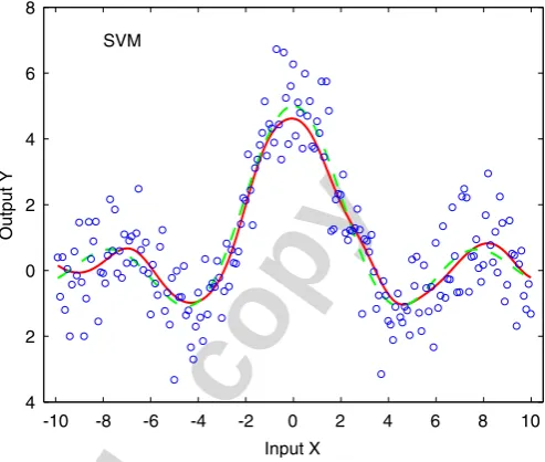
learning hyperparameters in the influence of the model generalisation capability. When one chooses a particular optimiser to solve the constrained quadratic programming (QP) of the SVM learning problem, for example, one also needs to assign some optimisation algorithmic parameters. These QP optimiser’s algorithmic parameters are similar in nature to the algorithmic parameters of the RWBS optimiser, and they are not the learning hyperparameters of the SVM algorithm. The learning hyperparameters of the SVM algorithm are the kernel variances2,Cand. Table 1

Summary of the experimental results for the simulated example

Algorithm SVM SESVM GSESVM

Kernel type Gaussian Gaussian Generalised Gaussian

Error band 0.2 0.3 0.2

RegularisationC 0.5 0.3 1.0

Model size 172 16 9

MSE over noisy training set

0.9522 0.9697 0.9658

MSE over noisy test set 1.2572 1.1950 1.2285 MSE over noise-free test

set

0.0740 0.0353 0.0344

-10 -8 -6 -4 -2 0 2 4 6 8 10 4

2 0 2 4 6 8

Input X

Output Y

SVM

Fig. 1. The experiment result of the SVM method for the simulated example. The circles are the noisy training data, the dashed curve is the sinc function, and the solid curve is the kernel model with 172 support vectors. The kernel variances2_{¼1, regularisation parameterC¼0:5 and}

error band parameter¼0:2.

-10 -8 -6 -4 -2 0 2 4 6 8 10 -4

-2 0 2 4 6 8

Input X

Output Y

SESVM

Fig. 2. The experiment result of the SESVM method for the simulated example. The circles are the noisy training data, the dashed curve is the sinc function, and the solid curve is the kernel model with 16 support vectors. The kernel variances2_{¼1, regularisation parameterC¼0:3 and}

error band parameter¼0:3.

Author's personal copy

4. Modelling experiments

A one-dimensional simulated example and three real data sets were used in our modelling experiments. For each example, three sets of results were obtained by the SVM, the SESVM and the GSESVM, respectively. The learning hyperparameters, C and , were optimised using grid search optimisation based on cross validation for each

algorithm. The single common kernel variances2_{, required}

for the SVM and SESVM algorithms, was similarly determined. The optimisation algorithmic parameters of the RWBS,PS,NG andMI, were chosen empirically.

Example 1. Two hundred points of training data fx;yg were generated from the scalar sinc function corrupted by an observation noise shown below

y¼5 sinx

x þZ, (37)

where the equally spaced inputx2 ½10;10andZdenotes the Gaussian white noise process with unit variance. A separate noisy test data containing 200 data samples was provided for model validation purpose. Two hundred points of noise-free data were also generated as the additional test data set. For the Gaussian kernel modelling, the common kernel variance was set tos2_{¼1. This value}

was found empirically to be appropriate. The error band

0 50 100 150 200 250 300 350 400 450 4

5 5.5 6

System input

Sample

0 50 100 150 200 250 300 350 400 450 3

4 5

System output

Sample 4.5

3.5

2.5 3.5 4.5 (a)

(b)

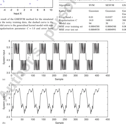
Fig. 4. The engine data set: (a) system inputvðtÞand (b) system outputyðtÞ. Table 2

Summary of the experimental results for the engine data set

Algorithm SVM SESVM GSESVM

Kernel type Gaussian Gaussian Generalised Gaussian

Error band 0.01 0.0107 0.01

RegularisationC 14.0 1600.0 300.0

Model size 94 50 15

MSE over training set 0.0004388 0.0004548 0.0004586 MSE over test set 0.0004930 0.0004991 0.0004894 -10 -8 -6 -4 -2 0 2 4 6 8 10

-4 -2 0 2 4 6 8

Input X

Output Y

GSESVM

Fig. 3. The experiment result of the GSESVM method for the simulated example. The circles are the noisy training data, the dashed curve is the sinc function, and the solid curve is the generalised kernel model with nine support vectors. The regularisation parameterC¼1:0 and error band parameter¼0:2.

Author's personal copy

parameter and regularisation parameter C for each algorithm were determined by grid search to minimise the MSE over the noisy test data set. The algorithmic

parameters of the RWBS were chosen empirically. The experimental results obtained by the SVM, SESVM and GSESVM methods are summarised inTable 1. Judging by

0 50 100 150 3

4 5

System/Prediction

0 100 200 300 3

4 5

System/Prediction

0 50 100 150 -0.05

0 0.05

Prediction error

0 100 200 300 -0.05

0 0.05

Prediction error

2.5 3.5 4.5

3.5 4.5

2.5

Sample Sample

Sample Sample 0.1

-0.1 -0.1

0.1

(a) (c)

(b) (d)

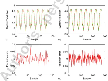
Fig. 5. The experiment result of the SVM method for the engine data set: (a) model prediction (green or light curve) superimposed on system output (red or dark curve); (b) model prediction error over the training set; (c) model prediction (green or light curve) superimposed on system output (red or dark curve); and (d) prediction error over the test set. The regularisation parameterC¼14:0, error band parameter¼0:01 and the model contains 94 kernels.

0 50 100 150 3

4 4.5 5

System/Prediction

0 100 200 300 3

4 5

System/Prediction

0 50 100 150 -0.05

0 0.05

Prediction error

0 100 200 300 -0.05

0 0.05

Prediction error

3.5

2.5

Sample

4.5

3.5

2.5

Sample

-0.1 0.1

Sample Sample

-0.1 0.1

(a) (c)

(b) (d)

Fig. 6. The experiment result of the SESVM method for the engine data set: (a) model prediction (green or light curve) superimposed on system output (red or dark curve); (b) model prediction error over the training set; (c) model prediction (green or light curve) superimposed on system output (red or dark curve); and (d) prediction error over the test set. The regularisation parameterC¼1600:0, error band parameter¼0:0107 and the model contains 50 kernels.

Author's personal copy

their MSE values over the noisy test data set, the three algorithms had similarly good generalisation capability but the model produced by the GSESVM method was the

sparsest containing only 9 kernels. The model maps derived by the three methods are depicted inFigs. 1–3, respectively, in comparison with the underlying sinc function.

0 50 100 150 3

4 5

(a)

System/Prediction

0 100 200 300 3

3.5 4 5

(c)

System/Prediction

0 50 100 150 0

0.05

(b)

Prediction error

0 100 200 300 -0.05

0

(d)

Prediction error

0.05

-0.1 0.1

Sample Sample

-0.1 -0.05 0.1

Sample 2.5

3.5 4.5

2.5 4.5

Sample

Fig. 7. The experiment result of the GSESVM method for the engine data set: (a) model prediction (green or light curve) superimposed on system output (red or dark curve); (b) model prediction error over the training set; (c) model prediction (green or light curve) superimposed on system output (red or dark curve); and (d) prediction error over the test set. The regularisation parameterC¼300:0, error band parameter¼0:01 and the model contains 15 kernels.

0 50 100 150 200 250 300 45

50 55 60 65

Sample

System output

0 50 100 150 200 250 300 3

2 1 0 1 2 3

Sample

System input

(a)

(b)

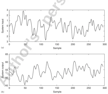
Fig. 8. The gas furnace data set: (a) system inputvðtÞand (b) system outputyðtÞ. X.X. Wang et al. / Neurocomputing 70 (2006) 462–474

Author's personal copy

Example 2. This example constructed a model representing the relationship between the fuel rack position (input vðtÞ) and the engine speed (output yðtÞ) for a Leyland TL11 turbocharged, direct injection diesel engine operated at low engine speed. The data set, depicted in Fig. 4, contained 410 samples. The study[3]has shown that this data set can be modelled as

yi¼FSðxiÞ þei, (38)

where yi¼yðiÞ and xi¼ ½yði1Þvði1Þvði2ÞT, FSðÞ

describes the unknown underlying system to be identified andeidenotes the system noise. It is often claimed that the

SVM method is capable of constructing sparse models with excellent generalisation performance with a small training set. We constructed the training set by using the data pairs ðxi;yiÞ for i¼3;6;9;12;. . . and putting rest of the data

pairs into the test set. Thus, the training set containedN¼

136 points, while the test set had 272 samples. The values of the single common kernel variances2_{for the two Gaussian}

kernel modelling cases were determined using a grid search, and the appropriate values were found to be 1.69 for the SVM algorithm and 2.60 for the SESVM algorithm, respectively.

Again, the error band parameter and regularisation parameterCfor each algorithm were found by grid search to minimise the MSE over the test data set. The algorithmic parameters of the RWBS were determined empirically.

Table 2 summarises the experimental results obtained by the SVM, SESVM and GSESVM algorithms. It can be seen that the GSESVM method produced the best result, in terms of model generalisation capability and model size.

Fig. 5 depicts the model prediction y^_i and the prediction error e^i¼yiy^i obtained by the SVM model over both

the training and test sets. Similarly, the modelling results of the SESVM and GSESVM algorithms are shown inFigs. 6

and7, respectively.

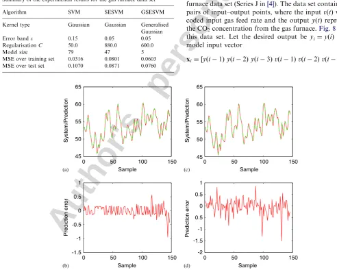
Example 3. This example constructed a model for the gas furnace data set (Series J in[4]). The data set contained 296 pairs of input–output points, where the inputvðtÞwas the coded input gas feed rate and the output yðtÞ represented the CO2concentration from the gas furnace.Fig. 8depicts

this data set. Let the desired output be y_i¼yðiÞ for the model input vector

xi¼ ½yði1Þyði2Þyði3Þvði1Þvði2Þvði3ÞT

(39) Table 3

Summary of the experimental results for the gas furnace data set

Algorithm SVM SESVM GSESVM

Kernel type Gaussian Gaussian Generalised Gaussian

Error band 0.15 0.05 0.05

RegularisationC 50.0 880.0 600.0

Model size 79 47 5

MSE over training set 0.0316 0.0801 0.0603 MSE over test set 0.1070 0.0871 0.0760

0 50 100 150 45

50 55 60 65

(a)

System/Prediction

0 50 100 150 45

50 55 60 65

(c)

System/Prediction

0 50 100 150 -1

0 1

(b)

Prediction error

0 50 100 150 -2

-1 0 1

(d)

Prediction error

Sample Sample

Sample Sample 0.5

-0.5

-1.5

-1.5 0.5 0.5

Author's personal copy

0 50 100 150 45

50 55 60 65

(a)

System/Prediction

0 50 100 150 45

50 55 60 65

(c)

System/Prediction

0 50 100 150 1

0 1

(b)

Prediction error

0 50 100 150 2

1 0 1

(d)

Prediction error

Sample Sample

0.5

-0.5

-1.5

Sample Sample

0.5

-0.5

-1.5

Fig. 10. The experiment result of the SESVM method for the gas furnace data set: (a) model prediction (green or light curve) superimposed on system output (red or dark curve); (b) model prediction error over the training set; (c) model prediction (green or light curve) superimposed on system output (red or dark curve); and (d) prediction error over the test set. The regularisation parameterC¼880:0, error band parameter¼0:05 and the model contains 47 kernels.

0 50 100 150 45

50 55 60 65

(a)

System/Prediction

0 50 100 150 45

50 55 60 65

(c)

System/Prediction

0 50 100 150 0

1

(b)

Prediction error

0 50 100 150 0

1

(d)

Prediction error

Sample Sample

Sample Sample

0.5

-0.5

-1

-1.5

0.5

-0.5

-1

-1.5

-2

Fig. 11. The experiment result of the GSESVM method for the gas furnace data set: (a) model prediction (green or light curve) superimposed on system output (red or dark curve); (b) model prediction error over the training set; (c) model prediction (green or light curve) superimposed on system output (red or dark curve); and (d) prediction error over the test set. The regularisation parameterC¼600:0, error band parameter¼0:05 and the model contains 5 kernels.

Author's personal copy

training set while the odd points were selected as the test set. For the Gaussian kernel modelling, an appropriate value for the single common kernel variance was found empirically to bes2_{¼20. The error band parameterand}

regularisation parameter C for each algorithm were determined by grid search to minimise the MSE over the test data set. The algorithmic parameters of the RWBS were set empirically.Table 3gives the experimental results obtained by the SVM, SESVM and GSESVM algorithms. The modelling results are also plotted in Figs. 9–11, respectively, for the three algorithms. It is clear that for this example the best result was obtained by the GSESVM method.

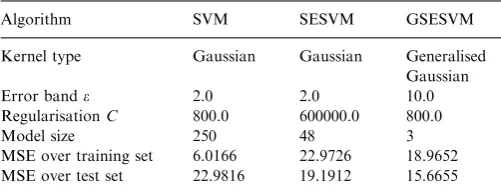
Example 4. This is a popular regression benchmark data set, Boston Housing, available at the UCI repository [21]. The data set comprises 506 data points with 14 variables. The task was to predict the median house value from the remaining 13 attributes. The first 456 data points from the data set were used for training and the remaining 50 data points were used to form the test set. As usual, the appropriate value for the single common kernel variance, required by the Gaussian kernel modelling, was determined via cross validation, yielding s2¼2116:0 ands2¼2025:0 for the SVM and SESVM, respectively. The error band parameter and regularisation parameter C for each algorithm were chosen by grid search via cross validation. The algorithmic parameters of the RWBS were set empirically. Table 4 summarises the modelling results for this data set. The results of Table 4 again show that the GSESVM method produced the best model, in terms of model generalisation performance and model size.

5. Conclusions

In this paper, we have first considered an alternative SVM formulation, referred to as the ESVM method, which does not assume the reproducing kernel Hilbert space and is capable of applying to non-Mercer kernels. Secondly, we have proposed a sparse kernel model construction algorithm, called the SESVM. In this approach, a parsimonious representation is selected using the standard OLS forward selection procedure and the corresponding model weights are then computed using the ESVM formulation. Thirdly, which

is a major contribution of our work, we have developed the generalised kernel modelling in which each kernel regressor has its tunable centre vector and diagonal covariance matrix. An orthogonal forward selection procedure has been proposed to construct a sparse generalised kernel model representation. At each model construction stage, a kernel regressor is optimised using a global optimisation search algorithm. Again the corresponding model weights are then calculated using the ESVM formulation, and this novel generalised kernel construction algorithm has been referred to as the GSESVM method. Our modelling experimental results have clearly demonstrated that both the SESVM and GSESVM methods compare favourably with the standard SVM formulation in terms of producing sparse models that generalise well. The GSESVM method has been shown to be particularly effective in constructing very sparse models with excellent generalisation capability, and we believe that it offers a state-of-the-art technique for regression modelling.

References

[1] H. Akaike, A new look at the statistical model identification, IEEE Trans. Autom. Control AC-19 (1974) 716–723.

[2] N. Aronszajn, Theory of reproducing kernels, Trans. Am. Math. Soc. 68 (1950) 337–404.

[3] S.A. Billings, S. Chen, R.J. Backhouse, The identification of linear and non-linear models of a turbocharged automotive diesel engine, Mech. Syst. Signal Process. 3 (2) (1989) 123–142.

[4] G.E.P. Box, G.M. Jenkins, Time Series Analysis, Forecasting and Control, Holden Day, San Francisco, CA, 1976.

[5] L. Breiman, Prediction games and arcing algorithms, Neural Comput. 11 (7) (1999) 1493–1518.

[6] O. Chapelle, V. Vapnik, O. Bousquet, S. Mukherjee, Choosing multiple parameters for support vector machines, Mach. Learn. 46 (1–3) (2002) 131–159.

[7] S. Chen, S.A. Billings, W. Luo, Orthogonal least squares methods and their application to non-linear system identification, Int. J. Control 50 (5) (1989) 1873–1896.

[8] S. Chen, C.F.N. Cowan, P.M. Grant, Orthogonal least squares learning algorithm for radial basis function networks, IEEE Trans. Neural Networks 2 (2) (1991) 302–309.

[9] S. Chen, X. Hong, C.J. Harris, Sparse kernel regression modelling using combined locally regularized orthogonal least squares and D-optimality experimental design, IEEE Trans. Autom. Control 48 (6) (2003) 1029–1036.

[10] S. Chen, X. Hong, C.J. Harris, P.M. Sharkey, Sparse modelling using orthogonal forward regression with PRESS statistic and regulariza-tion, IEEE Trans. Syst. Man Cybern. Part B 34 (2) (2004) 898–911. [11] S. Chen, B.L. Luk, Adaptive simulated annealing for optimization in signal processing applications, Signal Process. 79 (1) (1999) 117–128. [12] S. Chen, X.X. Wang, C.J. Harris, Experiments with repeating weighted boosting search for optimization in signal processing applications, IEEE Trans. Syst. Man Cybern. Part B 35 (4) (2005) 682–693.

[13] S. Chen, Y. Wu, B.L. Luk, Combined genetic algorithm optimisation and regularised orthogonal least squares learning for radial basis function networks, IEEE Trans. Neural Networks 10 (5) (1999) 1239–1243.

[14] N. Cristianini, J. Shawe-Taylor, An Introduction to Support Vector Machines: and Other Kernel-Based Learning Methods, Cambridge University Press, Cambridge, UK, 2000.

[15] K. Duan, S.S. Keerthi, A.N. Poo, Evaluation of simple performance measures for tuning SVM hyperparameters, Neurocomputing 51 (2003) 41–59.

Table 4

Summary of the experimental results for the Boston housing data set

Algorithm SVM SESVM GSESVM

Kernel type Gaussian Gaussian Generalised Gaussian

Error band 2.0 2.0 10.0

RegularisationC 800.0 600000.0 800.0

Model size 250 48 3

MSE over training set 6.0166 22.9726 18.9652 MSE over test set 22.9816 19.1912 15.6655

Author's personal copy

on-line learning and an application to boosting, J. Comput. Syst. Sci. 55 (1) (1997) 119–139.

[17] D.E. Goldberg, Genetic Algorithms in Search, Optimization and Machine Learning, Addison-Wesley, Reading, MA, 1989.

[18] S. Gunn, Support vector machines for classification and regression, Technical Report, ISIS Research Group, Department of Electronics and Computer Science, University of Southampton, UK, May 1998. [19] X. Hong, C.J. Harris, Nonlinear model structure design and construction using orthogonal least squares and D-optimality design, IEEE Trans. Neural Networks 13 (5) (2002) 1245–1250.

[20] X. Hong, C.J. Harris, S. Chen, P.M. Sharkey, Robust nonlinear model identification methods using forward regression, IEEE Trans. Syst. Man Cybern. Part A 33 (4) (2003) 514–523.

[21] hhttp://www.ics.uci.edu/mlearn/MLRepository.htmli.

[22] L. Ingber, Simulated annealing: practice versus theory, Math. Comput. Modeling 18 (11) (1993) 29–57.

[23] I.J. Leontaritis, S.A. Billings, Model selection and validation methods for non-linear systems, Int. J. Control 45 (1) (1987) 311–341. [24] K.F. Man, K.S. Tang, S. Kwong, Genetic Algorithms: concepts and

Design, Springer, London, 1998.

[25] R. Meir, G. Ra¨tsch, An introduction to boosting and leveraging, in: S. Mendelson, A. Smola (Eds.), Advanced Lectures in Machine Learning, Springer, Berlin, 2003, pp. 119–184.

[26] C.S. Ong, A.J. Smola, R.C. Williamson, Hyperkernels, Neural Informa-tion Processing Systems, vol. 15, MIT Press, Cambridge, MA, 2002. [27] B. Scho¨lkopf, A.J. Smola, Learning with Kernels: support vector

machines, regularization, optimization, and beyond, MIT Press, Cambridge, MA, 2002.

[28] B. Scho¨lkopf, A.J. Smola, R.C. Williamson, P.L. Bartlett, New support vector algorithms, Neural Comput. 12 (5) (2000) 1207–1245. [29] B. Scho¨lkopf, K.K. Sung, C.J.C. Burges, F. Girosi, P. Niyogi, T. Poggio, V. Vapnik, Comparing support vector machines with Gaussian kernels to radial basis function classifiers, IEEE Trans. Signal Process. 45 (11) (1997) 2758–2765.

[30] R.E. Schapire, The strength of weak learnability, Mach. Learn. 5 (2) (1990) 197–227.

[31] V. Vapnik, The Nature of Statistical Learning Theory, Springer, New York, 1995.

Xunxian Wangreceived his Ph.D. degree in the control theory and application field from Tsin-ghua University, Beijing, China, in July 1999.

From August 1999 to August 2001, he was a postdoctoral researcher in the State Key Labora-tory of Intelligent Technology and Systems, Beijing, China. From September 2001 to Decem-ber 2004, he was a research fellow at the University of Portsmouth, Portsmouth, UK. From January 2005, he has been a research fellow at Neural Computing Research Group, Aston University, Birmingham, UK. Dr. Wang’s main interests are in machine learning and neural networks, control theory and systems as well as robotics.

Sheng Chenreceived his Ph.D. degree in control engineering from the City University, London, UK, in 1986.

He joined the School of Electronics and Computer Science, University of Southampton, Southampton, UK, in September 1999. He previously held research and academic appoint-ments at the University of Sheffield, Sheffield, the University of Edinburgh, Edinburgh, and the University of Portsmouth, Portsmouth, all in UK. Professor Chen’s research works include wireless communications, machine learning and neural networks, finite-precision digital controller design, and evolutionary computation methods. He has published over 260 research papers.

In the database of the world’s most highly cited researchers, compiled by Institute for Scientific Information (ISI) of the USA, Dr. Chen is on the list of the highly cited researchers in the engineering category.

David Lowehas held the Chair of Neural Computing at Aston University, UK, since 1994. He is a co-inventor of the Radial Basis Function neural network architecture, and the NeuroScale model for data visualisation. His current research activities relate to stochastic generative control, biomedical applications of statistical pattern processing focussing on DNA microarrays and EEG/MEG brain signal analysis, and nonlinear methods for digital steganography.

Chris Harrisreceived his Ph.D. degree from the University of Southampton, Southampton, UK. He previously held appointments at the Uni-versity of Hull, Hull, the UMIST, Manchester, the University of Oxford, Oxford, and the University of Cranfield, Cranfield, all in UK, as well as being employed by the UK Ministry of Defence. He returned to the University of Southampton as the Lucas Professor of Aero-space Systems Engineering in 1987 to establish the Advanced Systems Research Group and, more recently, Image, Speech and Intelligent Systems Group. His research interests lie in the general area of intelligent and adaptive systems theory and its application to intelligent autonomous systems such as autonomous vehicles, manage-ment infrastructures such as command and control, intelligent control, and estimation of dynamic processes, multi-sensor data fusion, and systems integration. He has authored and co-authored 12 research books and over 400 research papers, and he is the associate editor of numerous international journals.

Dr. Harris was elected to the Royal Academy of Engineering in 1996, was awarded the IEE Senior Achievement medal in 1998 for his work in autonomous systems, and the highest international award in IEE, the IEE Faraday medal, in 2001 for his work in intelligent control and neurofuzzy systems.