Calculation of guided wave interaction with nonlinearities and generation of harmonics in composite structures through a wave finite element method

Calculation of guided wave interaction with nonlinearities and generation of

harmonics in composite structures through a wave finite element method

D. Chronopoulosa

a_{Institute for Aerospace Technology & The Composites Group, The University of Nottingham, NG7 2RD, UK}

Abstract

The extensive usage of composite materials in modern industrial applications implies a great range of possible

struc-tural failure modes for which the structure has to be frequently and thoroughly inspected. Nonlinear guided wave

inspection techniques have been continuously gaining attention during the last decade. This is primarily due to their

sensitivity to very small sizes of localised damage. A number of complex transformation phenomena take place when

an elastic wave impinges on a nonlinear segment, including the generation of higher and sub-harmonics. Moreover, the

transmission and reflection coefficients of each wave type become amplitude dependent. In this work, a generic Finite

Element (FE) based computational scheme is presented for quantifying guided wave interaction effects with Localised

Structural Nonlinearities (LSN) within complex composite structures. Amplitude dependent guided wave reflection,

transmission and conversion is computed through a Wave and Finite Element (WFE) method. The scheme couples

wave propagation properties within linear structural waveguides to a LSN and is able to compute the generation of

higher and sub-harmonics through a harmonic balance projection. A Newton-like iteration scheme is employed for

solving the system of nonlinear differential equations. Numerical case studies are presented for waveguides coupled

through a joint exhibiting nonlinear mechanical behaviour.

Keywords: Wave Interaction with Damage, Finite Elements, Composite Structures, Nonlinear Ultrasound, Structural

nonlinearities

1. Introduction

Modern industrial structures are increasingly made of composite layered materials due to their well-known

ben-efits. Composite structures may however exhibit a great variety of structural failure modes (including delamination,

fibre breakage, matrix cracking and debonding) and must be frequently inspected in order to ensure continuous

struc-tural integrity. An increasing tendency within the Strucstruc-tural Health Monitoring (SHM) community is the ’shift to

the left’ maintenance strategy [1] for which the earliest possible detection of damage is important. When it comes

to the aeronautical industry, approximately 27% of an average modern aircraft’s lifecycle cost [2] is spent on

inspec-tion and repair. The use of ’offline’ structural inspection techniques currently leads to a massive reduction of the

Nomenclature

Aω,−

q ,Aω,

−

f Generalised displacement and force wave interaction coefficients for an incoming wave of frequencyω

M,CandK Mass, damping and stiffness matrices of the coupling element

D Dynamics Stiffness Matrix (DMS) of a waveguide’s modelled periodic segment

ℜ Real operator

R Transformation matrix

S Wave scattering coefficient matrix

T Wave propagation transfer matrix

T1, T2 Harmonic motion transformation matrices, functions ofτ

a+_{, a}− _{Amplitudes of waves moving towards and away of the coupling element}

f Forcing vector for an elastic waveguide

fNL Nonlinear force vector induced by the coupling element’s inherent inelastic behaviour

q Physical displacement vector for an elastic waveguide

z Physical displacement vector for the coupling element

Lx Dimension of a waveguide’s modelled periodic segment

L, R, I Left, right sides and interior indices

c Transmission coefficient

r Reflection coefficient

k Wavenumber

j Number of DoF on each cross-section of the periodic waveguide segment

h, H Harmonic index and total number of harmonics considered in the harmonic balance projection

Hm Index of the lowest subharmonic considered in the harmonic balance projection

n, N Waveguide index and total number of waveguides existing in the considered system

w, Wn Wave eigenvector index and total number of waves accounted for in waveguide n

s Periodic segment positioning index

t Time

Φhqω,+,Φhω,

−

q Grouped displacement eigenvectors for the positive and negative going elastic waves at frequency hω

Φhfω,+,Φ hω,−

f Grouped forcing eigenvectors for the positive and negative going elastic waves at frequency hω φq,φf Displacement and forcing eigenvectors

γ Propagation constant and eigenvalue of the wave propagation eigenproblem

τ Generalised time variable

ω Fundamental input angular frequency

aircraft’s availability and significant financial losses for the operator. The online nondestructive detection and

eval-uation of damage in industrial structural components is of paramount importance for monitoring the condition and

residual life estimation of in-service structures. Linear ultrasonic Guided Wave (GW) techniques have been widely

employed for this purpose. These techniques however are primarily sensitive to gross defects but much less sensitive

to micro-damage. Nonlinear acousto-ultrasonic techniques, have been steadily receiving increasing attention during

the last decade. Complex wave phenomena such as higher and subharmonic wave generation, nonlinear resonances

or mixed frequency response can be induced by the two principal sources of nonlinearity in the structural system,

namely nonlinear elasticity and contact nonlinearity.

Elastic wave distortion and generation of higher harmonics during propagation in nonlinear media has been

re-ported as early as in [3]. The first attempt for modelling wave interaction with nonlinear joints can be found in [4, 5]. It

has been widely demonstrated that nonlinear ultrasonic techniques can be successfully deployed for detecting cracks

as well as distributed structural deterioration (e.g. fatigue) [6, 7, 8, 9, 10, 11, 12]. The success of the developed

methods is based on predicting and measuring the nonlinearities-induced wave effects which are pronounced in

dam-aged and degraded structures but nearly unmeasurable in the undamdam-aged ones. A number of Nonlinear Elastic Wave

Spectroscopy (NEWS) approaches [13, 14, 15] have also been presented and proved capable of detecting the

pres-ence of damage of very small sizes (in the order of 0.1mm) in composite structures. Wave propagation and material

degradation detection in 1-D and 2-D media was investigated through a spring model in [16, 17]. A numerical scheme

for predicting nonlinear wave interaction with an interface of rough surfaces in contact was presented in [18]. The

non-collinear mixing of bulk shear waves investigated in [19] presented significant potential for assessing material

state than other nonlinear ultrasonic techniques because system nonlinearities can be both independently measured

and largely eliminated. The development of an analytical framework for modelling the multi-modal guided wave

interaction with damage was presented by the authors of [20, 21]. In [22], a numerical scheme was presented in order

to quantify the amplitude of the reflected compression and Rayleigh waves when impinging at the edge of an elastic

plate. In [23] the authors coupled linear to nonlinear FE segments and investigated wave interaction with damage in

3-D solid media by means of a Landau’s theory. Detection of fatigue damage in composite structures through higher

harmonics generations has also recently been reported [24]. The short reviews provided by the authors in [25, 26] are

informative on the general progress of nonlinear ultrasonics, while a comprehensive outline on the techniques

dedi-cated to predicting and measuring higher harmonic generation in metallic structures is presented in [27]. An inclusive

review on modelling wave-crack nonlinear interaction phenomena can be found in [28]. Despite the aforementioned

attempts to capture wave interaction with LSNs, there is currently no generic computational scheme for predicting

these quantities for composite layered structures.

The FE based wave propagation analysis within periodic structures was firstly considered in [29]. The wave

dispersion characteristics within the layered media can be accurately predicted for a very wide frequency range,

by solving a polynomial eigenvalue problem for the propagation constants to be sought. The work was extended

eigenproblem solutions and further improve the computational efficiency of the method. The vibration of a uniform

waveguide through the WFE technique was investigated in [32, 33]. The method was also employed in order to

predict the dynamic and vibroacoustic response [34, 35, 36] of layered structures. The same FE based approach has

been employed in order to compute the reflection and transmission coefficients of waves impinging on linear joints of

finite dimensions [37, 38].

In this work, a generic FE-based scheme for computing wave interaction with LSNs is presented for the first time.

Guided wave reflection, transmission and conversion is computed through a wave and finite element approach. The

scheme couples wave propagation properties within linear structural waveguides to a LSN and is able to determine the

generation higher and sub-harmonics for each wave type through a harmonic balance projection. The new approach

can predict reflections and transmissions at harmonic frequencies with a speed that is orders of magnitude faster than

conventional transient FE solutions. The structure can be of arbitrary complexity, layering and material characteristics

as FE modelling is employed. A Galerkin projection is used to transform the system of nonlinear differential

equa-tions of motion into a set of nonlinear algebraic equaequa-tions which is subsequently solved through a Newton’s iteration

method. The generation of wave harmonics, as well as amplitude-dependent wave reflection and transmission

coef-ficients are reported through the exhibited numerical case studies. This is the first approach that can accurately and

efficiently map the frequency-dependent interactions of guided waves with nonlinearities in complex structures.

The paper is organized as follows: In Sec.2 the formulation of the wave and finite element method for predicting

acoustic and ultrasonic GW interaction with LSNs is presented. A description of the Galerkin projection as well as

of the Newton’s iteration scheme employed for solving the system of nonlinear differential equations is also given. In

Sec.3 the proposed method is validated for two different waveguides through comparison to full transient FE analyses.

Conclusions on the presented work are given in Sec.4.

2. Elastic wave interaction with structural nonlinearities

2.1. Computing wave propagation in a layered structure through a wave and finite element method

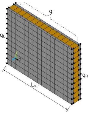
Elastic wave propagation is considered in the x direction of the linear layered waveguide of Fig.1. The problem

can be condensed using a transfer matrix approach as in [31]. The frequency dependent Dynamic Stiffness Matrix

(DMS) of the waveguide’s periodic segment can be partitioned with regard to its left/right sides and internal DoF as

                

DLL DLI DLR

DIL DII DIR

DRL DRI DRR

                                  qL qI qR                  =                  fL 0 fR                  (1)

with q the displacement and f the forcing vectors. Using a dynamic condensation for the internal DoF the problem

can be expressed as

         

DLL−DLID−_II1DIL DLR−DLID−_II1DIR

DRL−DRID−II1DIL DRR−DRID−II1DIR

q

q

q

L

Figure 1: Caption of the WFE modelled composite waveguide with the left and right side nodes qL, qRbullet marked. The range of interior nodes

qIis also illustrated.

Assuming that no external forces are applied on the segment the displacement continuity and force equilibrium

equa-tions at the interface of two consecutive periodic segments s and s+1 give

qs+1 L =q

s R

f_Ls+1=−f_Rs

(3)

Using Eqs.2,3 the relation of the displacements and forces of the left and right sides of the segment can be written as

        

qs_L+1

f_Ls+1         

=T         

qs_L

f_Ls         

(4)

and the expression of the symplectic transfer matrix T can be formulated

T=

         

D11 D12

D21 D22

         

[2 j×2 j]

(5)

with

D11=−(DLR−DLID−_II1DIR)−1(DLL−DLID−_II1DIL)

D12=(DLR−DLID−_II1DIR)−1

D21=−DRL+DRID−_II1DIL+

+(DRR−DRID−_II1DIR)(DLR−DLID_II−1DIR)−1(DLL−DLID−_II1DIL)

D22=−(DRR−DRID−II1DIR)(DLR−DLID−II1DIR)−1

With a wave propagating freely along the x direction, the propagation constantγ = e−ikLx _{relates the right and left}

nodal displacements and forces by

qs R=γq

s L

fs R=−γf

s L

(7)

By substituting Eqs.3,7 in Eq.4, the free wave propagation is described by the eigenproblem

γ         

q_Ls

f_Ls          =T         

qs_L

f_Ls          (8)

whose eigenvaluesγw and eigenvectors φw =

         φq φf          w

solution sets provide a comprehensive description of the

propagation constants and the wave mode shapes for each of the elastic waves propagating in the structural waveguide

at a specified angular frequencyω. Both positive going (withγ+_wandφ_w+) and negative going waves (γ_w−andφ−_w) are

sought through the eigensolution. Positive going waves are characterised [38] by

|γ+w|≤1,

ℜ(iωφ+_f⊤φ+q)<0 if|γ+w|=1

(9)

stating that when a wave is travelling in the positive x direction its amplitude should be decreasing, or that if its

amplitude remains constant (in the case of propagating waves with complete absence of attenuation), then there is

time averaged power transmission in the positive direction.

2.2. Wave interaction with linear localised structural inhomogeneities

The layered and periodic in the x direction waveguide of Fig.1 is hereby considered, with its propagation constants

for the elastic waves travelling in the x direction sought as described in Sec.2.1. For the sake of progressive

presen-tation of the approach, we are initially assuming a system of two waveguides connected through a linear structural

coupling element which is entirely FE modelled and which has different mechanical characteristics than the ones of

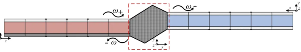
the two waveguides coupled to it. A depiction of the system is presented in Fig.2. As already stated, each waveguide

can be of different layering and can also support a different number Wnof propagating waves at a given angular

fre-quencyω. An extensive description of how to deal with waveguides having different layouts and meshes can be found

in [37]. Each supported wavemode w with w∈[1· · ·W1] for waveguide 1 in the system can be grouped as

Φ+1,q=

φ+_q,1 φ+_q,2 · · · φ+_q,W 1

Φ+

1,f =

φ+_f,1 φ+_f,2 · · · φ+_f,W 1

Φ−1,q=

φ−_q,1 φ−_q,2 · · · φ−_q,W 1

Φ−1,f =

φ−_f,1 φ−_f,2 · · · φ−_f,W1

(10)

with each matrix being of dimension [ j×W1]. Similarly the equivalent expressions for waveguide 2 (i.e.Φ+

2,q,Φ

+

2,f,Φ

−

2,q,Φ

−

2,f)

can be obtained with eigenvectors being normalised to unity. The wave modes of the entire system can be computed

Figure 2: Periodic elastic waveguides connected through a coupling element exhibiting inhomogeneous but linear mechanical behaviour. Coupling

element is depicted in the highlighted frame and is entirely FE modelled. A positive going wave+of angular frequencyωimpinging on the

coupling element will give rise to reflected and transmitted outgoing−waves of the same frequency.

for the fundamental excitation frequencyωand be grouped as

Φ+q =

         

Φ+1,q 0

0 Φ+2,q

         

(11)

with similar expressions standing forΦ+

f,Φ

−

q, Φ

−

f. Assuming that the two waveguides have the same number of

degrees of freedom j at their interfaces and that the same number of waves is retained for both of them in the wave

basis, then the size of the above table will be [2 j×2W]. For each waveguide, the local coordinate system is defined

such that the waveguide’s axis is directed towards the joint (direction+). The rotation matrix Rn transforms the

DoFs from the local to the global coordinates of the system. For the two-waveguide system, rotation matrices can be

grouped in a block diagonal matrix R as

R=

         

R1 0

0 R2

         

[2 j×2 j]

(12)

The equation of motion for the linear, FE modelled coupling element can be in general written as

M_¨z(t)+C_˙z(t)+Kz(t)=fext(t) (13)

with fext(t) being the external forces applied to the coupling element by the two waveguides. The continuity conditions

for the element give

z(t)=Rq(t) (14)

with q=[q⊤₁q⊤₂]⊤_{[2 j×1]}. The equilibrium at the coupling element gives

fext(t)−Rf(t)=0 (15)

with f(t) the set of forces applied by the impinging and outgoing waves to the coupling element.

2.2.1. Calculation of the wave scattering matrix

Waves of the fundamental excitation frequencyωhaving amplitudes aω,₁+are impinging on the coupling element from the side of waveguide 1. Their interaction with the coupling element will give rise to reflected waves of

ampli-tudes aω,₁−=rω

1,1a

ω,+

1 in waveguide 1, while they also give rise to transmitted waves of amplitudes a

ω,−

2 =c

ω

2,1a

ω,+

the second waveguide with rω_1,1and cω_2,1being matrices containing the reflection and transmission coefficients of the coupling element at frequencyω. These coefficients define the wave scattering matrix Sω_{of the joint, whose partitions}

relate the amplitudes of the incident and scattered waves as

aω,−=Sωaω,+ (16)

with aω,_[2W+_×1]the vector containing the amplitudes of the incoming waves moving towards the coupling element and aω,_[2W−_×1] the vector containing the amplitudes of the reflected and transmitted outgoing waves. The wave scattering matrix Sωfor the two-waveguide linear system can be written as

Sω=                                 

r1,1 · · · c1,W · · · c1,2W

· · · ·

cW,1 · · · rW,W · · · cW,2W

· · · ·

c2W,1 · · · c2W,W · · · r2W,2W

                                 ω

[2W×2W]

(17)

which can be computed for the selected range of harmonics of the fundamental frequencyω. The motion of the

waveguides in the physical 3D coordinate system is described in terms of displacements q and forces f. On the other

hand, in the wave domain the same motion can be described as a linear superposition of the retained propagating wave

vectorsΦω,n,q+−,Φ

ω,+−

n,f along with their amplitudes a

ω,+_{and a}ω,−_{. This superposition can be expressed as}

qn(t)=Φω,n,q+aω,n+cos(ωt)+Φω,

−

n,qaω,

−

n cos(ωt)

fn(t)=Φω,_n,+_faω,n+cos(ωt)+Φω,

−

n,fa

ω,−

n cos(ωt)

(18)

and by concatenating the corresponding vectors and matrices the general expressions for q and f for the system of

waveguides can be expressed as

q(t)=Φω,q+aω,+cos(ωt)+Φω,q−aω,−cos(ωt)

f(t)=Φω,f+a

ω,+_cos(ωt)+ Φω,f−a

ω,−_cos(ωt) (19)

It is noted that sin terms are not included in the above expansions as the phase of each wave scattering coefficient is

captured by the imaginary part of the sought interaction coefficients aω,−_{. By performing the convenient substitution} τ=ωt and grouping the trigonometric terms the following expression can be acquired

q(τ)=Φω,q+T2aω,++T1Aω,

−

q (20)

with T2(τ)=

         

cosτ 0

0 cosτ

         

, T1(τ)=diag(cosτ)[2 j×2 j] andA

ω,−

q being the generalised displacement wave

inter-action coefficient vector written as

Aω,q−=

Φω,q−Sωaω,+

[2 j×1]

(21)

The following expressions can be immediately derived

f(τ)=_Φω,_f+T2aω,++T1Aω,

−

f

˙q(τ)=ωΦω,q+

dT2

dτ a

ω,+_+ωdT1

dτ A

ω,−

q

¨q(τ)=ω2

Φω,q+

d2T2

dτ2 a

ω,+_+ω2d 2_T

1

dτ2 A

ω,−

q

(22)

withAω,_f−formulated similarly toAω,q−. Substituting Eqs.20,22 into Eqs.14,15 and then into Eq.13 gives the

gener-alised expression for the equation of motion of the coupling element

ω2_MR

Φω,q+

d2T2

dτ2 a

ω,+_+ω2_MRd 2_T

1

dτ2 A

ω,−

q +ωCRΦ

ω,+

q

dT2

dτ a

ω,+₊

+ωCRdT1 dτ A

ω,−

q +KRΦ

ω,+

q T2aω,++KRT1Aω,q−=RΦ

ω,+

f T2a

ω,+_+RT

1Aω,_f −

(23)

A set of equations with the transmission and reflection coefficients as unknowns can be obtained through a Galerkin

projection of Eq.23 as

2π

R

0

" T⊤₁

"

ω2_MRd 2_T

1

dτ2 +ωCR

dT1

dτ +KRT1 #

Aω,q−−T⊤1RT1Aω,

−

f

# dτ+

2π

R

0

T⊤₁ "

ω2M_RΦω,_q+d

2_T 2

dτ2 +ωCRΦ

ω,+

q

dT2

dτ +KRΦ

ω,+

q T2−RΦω,_f+T2

#

aω,+_dτ=0

(24)

A Newton’s iterative scheme can be eventually employed in order to extract the wave interaction coefficients Sωout of Eq.24 by exciting one by one the incoming waves for each waveguide (that is by setting all wave amplitudes in aω,+ to zero except for the investigated incoming wave). As no matrix inverse is involved for the computation of the wave

interaction coefficients (in contrast to [38]), a reduced wave basis can be retained without ill-conditioning of the above

expressions. It should be stressed that modelling non-conservative waveguides and coupling elements implies that all

computed wavenumbers will be complex and the strict distinction between evanescent and propagating waves breaks

down. In that case, an extended wave basis should be retained (all waves having a non-negligible real wavenumber

part should be kept) in order to take into account for wave conversions induced by material damping. In most practical

situations however, the assumption of a conservative coupling element yields reliable results for the wave interaction

coefficients as discussed in [39].

2.3. Wave interaction with structural nonlinearities

It is hereby assumed that the modelled coupling element exhibits a specific and known nonlinear mechanical

behaviour. It is still given that an incident wave of fundamental frequencyωis impinging on the coupling element,

however this localised nonlinearity in the system will give rise to a number of waves of super-harmonic (hω) and

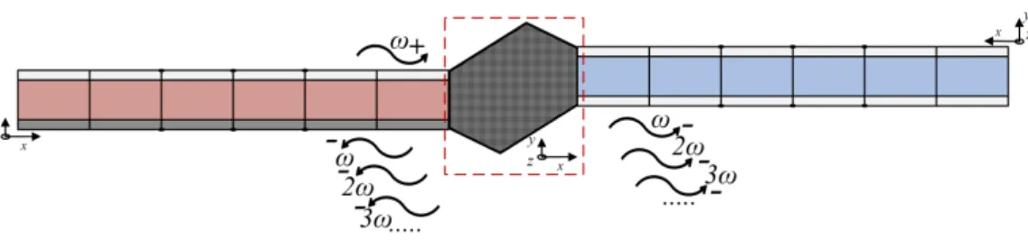
sub-harmonic (ω/h) frequencies during the interaction process (see Fig.3). The wave basis for each waveguide can

be computed and grouped as in Eq.11, however in order to project wave motion in multiple sub-harmonics and

Figure 3: Periodic elastic waveguides connected through a coupling element exhibiting inelastic mechanical behaviour. A positive going wave+_of

angular frequencyωimpinging on the coupling element will give rise to reflected and transmitted outgoing−waves of multiple subharmonic and

superharmonic frequencies.

of higher harmonics H and subharmonics Hmto be computed and included in the wave basis depends on the order

of nonlinearity of the modelled coupling element (see also [20, 21]). Therefore each supported wavemode w with

w ∈ [1· · ·Wn] for each waveguide in the system has to be computed for the super and sub-harmonics hω with

h∈[1/Hm· · ·1· · ·H] and be grouped as

Φhqω,+=

         

Φh1ω,,q+ 0

0 Φh2ω,,q+

         

[2 j×2W]

(25)

with similar expressions standing forΦhfω,+,Φ hω,−

q ,Φ hω,−

f . The equation of motion for the nonlinear, FE modelled

coupling element can now be generically written as

M_¨z(t)+C_˙z(t)+K_{z(t)+fNL=fext(t) (26)}

with fNLthe nonlinear force vector induced by the coupling element’s inherent inelastic behaviour. The same

conti-nuity and equilibrium conditions for the element are applied as expressed by Eqs.14,15. Waves of the fundamental

excitation frequencyωhaving amplitudes aω,n+are impinging on the coupling element from waveguide 1. For each

considered harmonic hω, they give rise to reflected waves of amplitudes ah₁ω,−=r₁hω_,1aω,₁+in the first waveguide, while they also generate transmitted waves of amplitudes ah₂ω,−=chω

2,1a

ω,+

1 in the second waveguide with r hω

1,1and c hω

2,1being

matrices containing the reflection and transmission coefficients of the coupling element at each harmonic hω. These

define the wave scattering matrix Shω_{of the joint}

ahω,−=Shωaω,+ (27)

which now has to be computed for each considered sub-harmonic and super-harmonic frequency. The wave scattering

matrix Shω_{now projects the incoming waves a}ω,+_{of fundamental frequencyωto each of the higher and sub-harmonics}

hω. The matrix can be computed for the selected range of harmonics of the fundamental frequencyω. Similarly to

Eq.18, a superposition expression can be written for the case where wave energy escapes towards higher and

sub-harmonics as

qn(t)=Φω,n,q+aω,n+cos(ωt)+ H

P

h=1Φ hω,−

n,q ahω,

−

n cos(hωt)+ Hm

P

h=2Φ hω,−

n,q ahω,

−

n cos(h1ωt)

fn(t)=Φω,_n,f+aω,n+cos(ωt)+ H

P

h=1Φ hω,−

n,f a hω,−

n cos(hωt)+ Hm

P

h=2Φ hω,−

n,f a hω,−

n cos(1hωt)

(28)

and by concatenating the corresponding vectors and matrices the general expressions for q and f for the system of

waveguides can be expressed as

q(t)=_Φω,q+aω,+cos(ωt)+ H

P

h=1Φ hω,−

q ahω,−cos(hωt)+ Hm

P

h=2Φ hω,−

q ahω,−cos(1hωt)

f(t)=Φω,f+a

ω,+_cos(ωt)+PH

h=1Φ hω,−

f a

hω,−_cos(hωt)+HPm

h=2Φ hω,−

f a

hω,−_cos(1 hωt)

(29)

The above expressions can be employed to perform a cyclostationary projection of the behaviour of the system through

the Harmonic Balance Method (HBM) [40]. By performing the convenient substitutionτ = ωt once again and

grouping the trigonometric terms the following expression can be acquired

q(τ)=Φω,q+T2a++T1Aω,q− (30)

with T2(τ) expressed as in Sec.2.2 and T1(τ)=

h

diag(cosτ)[2 j×2 j],diag(cos 2τ)[2 j×2 j],· · ·,diag(cos Hτ)[2 j×2 j]

i

[2 j×2 jH],

whileAω,−

q is the generalised displacement wave interaction coefficient vector now written as

Aω,q−=

                                        

Φω,q−Sωaω,+

Φ2qω,−S2ωaω,+

· · ·

ΦqHω,−SHωaω,+

· · ·

Φ

1 Hmω,− q S

1 Hmω_aω,+

                                        

[2 jH×1]

(31)

The expressions of Eq.22 are still valid and Eq.23 for the generalised equation of motion of the coupling element is

now modified as

ω2_MR

Φω,q+

d2T2

dτ2 a

ω,+_+ω2_MRd 2_T

1

dτ2 A

ω,−

q +ωCRΦ

ω,+

q

dT2

dτ a

ω,+₊

+ωCRdT1 dτ A

ω,−

q +KRΦ

ω,+

q T2aω,++KRT1Aω,q−+fNL=RΦω,_f+T2aω,++RT1Aω,_f−

(32)

It is noted thatK_{in the above expression represents the elastic part of the mechanical behaviour of the coupling}

element. A set of nonlinear, algebraic equations can be obtained through a Galerkin projection [41] of Eq.32 back

onto the set of harmonic solutions as

2Hmπ

R

0

" T⊤₁

" ω2_MRd

2_T 1

dτ2 +ωCR

dT1

dτ +KRT1 #

Aω,−

q −T⊤1RT1A

ω,−

f

# dτ+

2Hmπ

R

0

T⊤₁ "

ω2_MRΦω,+

q

d2T2

dτ2 +ωCRΦ

ω,+

q

dT2

dτ +KRΦ

ω,+

q T2−RΦω,_f+T2

#

aω,+_dτ+

2Hmπ

R

0

T⊤₁fNLdτ=0

(33)

A Newton’s iterative scheme similar to the one employed in Sec.2.2 can be used to extract the wave interaction

coefficients Sω/Hm_{,· · ·S}ω_{, S}2ω_{,· · ·S}Hω_{out of Eq.33 by exciting one by one the incoming waves for each waveguide.}

Algorithm 1 Newton-like iterative scheme for computing the wave interaction coefficients for localised structural

nonlinearities

1: Set convergence criteria for the iterative process

2: Input the total number of investigated super-harmonics H and sub-harmonics Hm, the amplitudes of waves moving

towards the nonlinearity aω,+_{, the grouped displacement and force eigenvectors for the linear waveguidesΦ}hω,+

q ,

Φhqω,−,Φh_fω,+,Φhω,

−

f as well as the structural description of the nonlinear coupling elementM,C,Kand fNL

3: Input initially assumed complex values for the reflection and transmission coefficients under investigation

4: i←1 Substitute set of transmission and reflection coefficients in S, then computeAω,q−,Aω,

−

f

5: Numerically evaluate Eq.33

6: Numerically evaluate the Jacobian matrix of sensitivities for each wave interaction coefficient sought

7: if Sensitivity satisfies the corresponding convergence criterion then

8: Solution corresponds to a local minimum

9: if Value of Eq.33 satisfies the corresponding convergence criterion then

10: Solution corresponds to global solution of wave interaction coefficients and process can end

11: else

12: Radically alter the assumed interaction coefficients and go to Step 4

13: end if

14: else

15: Use Jacobian in order to alter the assumed reflection/transmisison coefficients for converging towards a local

minimum. i←i+1 (next solution step). Go to Step 4

16: end if

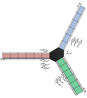
Figure 4: Periodic elastic waveguides connected through a coupling element exhibiting inelastic mechanical behaviour. A positive going wave+_of

angular frequencyωimpinging on the coupling element will give rise to reflected and transmitted outgoing−_{waves of multiple subharmonic and}

superharmonic frequencies.

2.4. Generalization to an arbitrary number of connected waveguides

The scheme presented in Sec.2.3 can be generalised to include more than two waveguides connected at the

nonlin-ear coupling element. In the general case, we are assuming a system of N waveguides as in Fig.4. As already stated,

each waveguide can be of different and arbitrary layering and can also support a different number Wnof propagating

waves at a given frequency. Each supported wavemode w with w∈[1· · ·Wn] for the nth waveguide in the system can

be grouped as

Φhnω,,q+=

φh_qω,_,1+ φ_qhω,_,2+ · · · φh_qω,_,W+

Φhnω,,f+=

φh_fω,_,1+ φh_fω,_,2+ · · · φh_fω,_,W+

Φhnω,,q−=

φh_qω,_,1− φ_qhω,_,2− · · · φh_qω,_,W−

Φhnω,,f−=

φh_fω,_,1− φh_fω,_,2− · · · φh_fω,_,W−

(34)

with each matrix being of dimension [ j×Wn]. The wavemodes of the entire system can be computed for each

waveguide n with n ∈ [1· · ·N] and for the fundamental excitation frequencyωas well as for the higher and

sub-harmonics hωwith h∈[1/Hm· · ·1· · ·H] and be grouped as

Φhqω,+=

                        

Φh1ω,,q+ 0 · · · 0

0 Φh2ω,,q+ · · · 0

· · · ·

0 0 · · · _Φhω,+

N,q

                        

[ jN×WN]

with similar expressions standing forΦhfω,+,Φ hω,−

q ,Φhω,

−

f . For each waveguide, the local coordinate system is defined

such that the waveguide’s axis is directed towards the joint (direction+). The rotation matrix Rntransforms the DoFs

from the local to the global coordinates of the system. Rotation matrices can be grouped in a block diagonal matrix R

as

R=

                        

R1 0 · · · 0

0 R2 · · · 0

· · · ·

0 0 · · · RN

                        

[ jN×jN]

(36)

The procedure then follows the same steps through Eq.26 to Eq.33 in order to sought the set of transmission and

re-flection coefficients for each harmonic frequency and each modelled waveguide when a single wave type is impinging

on the coupling element. The increase in the number of waveguides and the size of the concatenated wave basis can

radically increase the computational burden of the iterative solution scheme. Parallel computing algorithms can be

employed as the most straightforward tool to minimise the computational cost.

3. Numerical case studies

3.1. Validation of wave interaction coefficients through full FE simulations

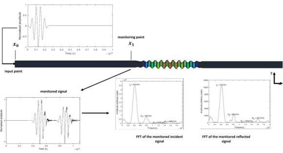
The above exhibited scheme will be validated through full FE transient simulations. The entire 1D structure

is modelled through linear, brick solid FE and the displacementsφω,_q,w+corresponding to a certain propagating wave mode w are imposed on one of its endsχ0 (see also Fig.5 for illustration). A Hanning-windowed signal containing

11 cycles is selected in order to minimise spectral leakage for the propagating packet. The displacements at a certain

monitoring cross-section of the waveguide laying before the LSN at distanceχ1, are recorded along with the incident

and reflected wave signatures. The reflection coefficient is defined as the ratio of energies of the reflected signal over

the incident one. These wave packet energies can effectively be computed through a Fourier transform over the time

ranges corresponding to wave incidence and reflection. The same transform can directly furnish the wave energies

at each generated sub-harmonic and super-harmonic. Transmission coefficients can be computed through the same

approach with the monitored cross-section laying after the LSN.

Spatial (element size) and temporal (integration time step) resolutions of the finite element model are chosen to

ensure solution convergence while ensuring the model computational size is reasonable. Time step is selected equal

to 1

20fmax

with fmax the maximum harmonic frequency considered in the problem. The element size is chosen equal

to λmin

20 whereλmin is the minimum wavelength to be taken into account in the wave basis (estimated through the computed wavenumbers from the wave and finite element scheme in Sec.2.1). This discretisation is adequate to avoid

spatial aliasing and ensure the inclusion of higher harmonics [42]. The smaller the integration time step dt, the better

the accuracy of the numerical result which however induces a greater computational cost.

x

&&dŽĨƚŚĞŵŽŶŝƚŽƌĞĚŝŶĐŝĚĞŶƚ ƐŝŐŶĂů

&&dŽĨƚŚĞŵŽŶŝƚŽƌĞĚƌĞĨůĞĐƚĞĚ ƐŝŐŶĂů

ŝŶƉƵƚƉŽŝŶƚ _y

࢞૙ ࢞૚

ŵŽŶŝƚŽƌĞĚƐŝŐŶĂů

ŵŽŶŝƚŽƌŝŶŐƉŽŝŶƚ

Figure 5: Schematic representation of the computation of reflection/transmission coefficients through a transient FE analysis. A Hanning windowed

signal is imposed on one end of the waveguide and the response is measured at monitoring cross-sectionχ1. The energy of each wave packet is

then calculated through a Fourier transform.

3.1.1. Projecting structural motion of a waveguide on its wave basis

The full FE simulations provide a complete description of the global displacements of a waveguide’s cross-section

as a function of time. In certain cases however wave conversion may take place at the point of the LSN. It is therefore

essential to decompose these global displacements into a sum of independent wave mode displacements using the

wave superposition principle. It is indeed helpful to note that once the wave displacement basis

Φ+n,q=

φ+_q,1 φ+_q,2 · · · φ+_q,W

(37)

for a certain composite waveguide has been determined through standard WFE computations, then any motion within

the structure can be described as a superposition of these wave mode shapes as

q+_n =Φω,n,q+a

ω,+ ₍₃₈₎

with aω,+the vector of amplitude coefficients denoting the participation of each wave type in the global waveguide motion and which can be obtained for each cross-section and each instant in time if the physical displacements q+n

are known through inverting the above expression (a pseudoinverse can be employed when a reduced wave basis is

kept andΦω,n,q+is not square). By registering aω,+as a function of time for a certain cross-section of the waveguide

and employing a Fourier transform, the frequency content for each wave type and subsequently the reflection and

transmission coefficients for each investigated wave motion is straightforward to obtain through the results of a full

3.2. Validation for an aluminium beam

The computational scheme exhibited above is initially applied in a discretized aluminium beam system as

pre-sented in Fig.6. The configuration comprises two waveguides having a cross-section of 8mm×12mm. The two

waveguides can in general have different characteristics however in this case they are both assumed to be made of

aluminium and are connected through a nonlinear element governed by a third order nonlinearity implemented within

the coupling element. A damping loss factor equal toη=1% was considered. By modelling the identical waveguides

through the WFE approach presented in Sec.2.1, it can be found that four waves can propagate within the structure.

Figure 6: Schematic representation of the two healthy and elastic monolayer waveguides (a) and (b) coupled through a nonlinear element (c).

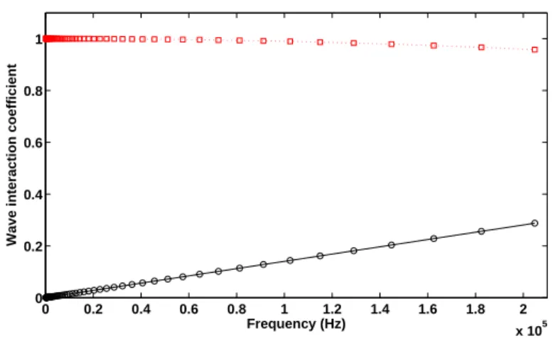
In order to validate the presented approach in the linear domain first, the results derived through Eq.24 are initially

compared against the methodology presented in [38] when a purely elastic coupling element is considered connecting

the two waveguides with Ece=Ewg/2 where Ece stands for the Young’s modulus of the coupling element and Ewgfor

the one of the waveguides. The results for this linearly softened coupling element using both approaches are presented

in Fig.7.

0 0.2 0.4 0.6 0.8 1 1.2 1.4 1.6 1.8 2 x 105 0

0.2 0.4 0.6 0.8 1

Frequency (Hz)

Wave interaction coefficient

Figure 7: Absolute values of the wave interaction coefficients for a linearly softened coupling element connecting the two waveguides: Reflection

coefficients for the pressure wave computed according to the current scheme (–), Reflection coefficients computed as in [38] (◦), Transmission

coefficients computed according to the current scheme (· · ·), Transmission coefficients computed as in [38] ().

Excellent agreement is observed for the reflection and transmission coefficients, while the interaction coefficients

for the higher and sub-harmonic outgoing waves are as expected null. A nonlinear coupling element is subsequently

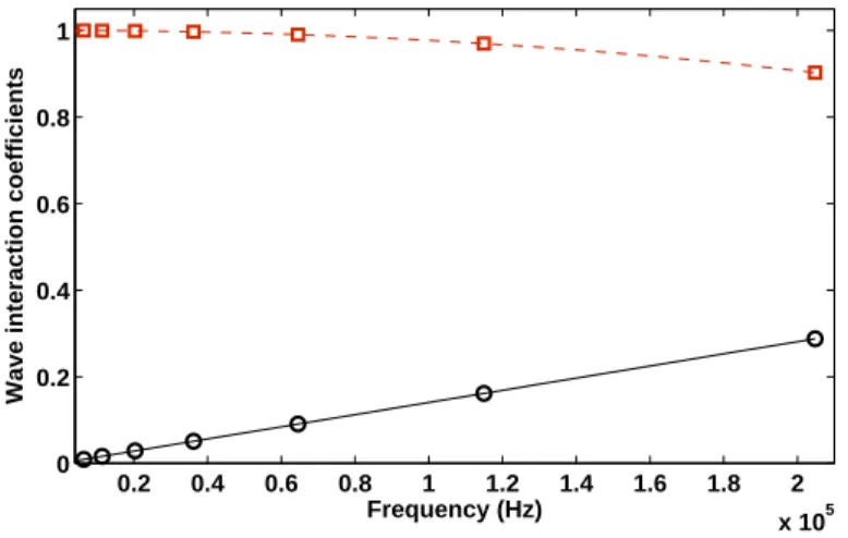
considered comprising a variable stiffness knl being dependent on the instantaneous deformation distance d. The

imposed amplitude of the incoming propagating wave is equal to 10µm. The results on the harmonic reflections

for a nonlinearly hardening element (computed through Eq.33) are presented below in Figs.8, 9. As expected and

demonstrated in Fig.9, the LSN gives rise to higher harmonic waves which are generally more pronounced at higher

excitation frequencies.

0.2 0.4 0.6 0.8 1 1.2 1.4 1.6 1.8 2

x 105 0

0.2 0.4 0.6 0.8 1

Frequency (Hz)

Wave interaction coefficients

Figure 8: Absolute values of the wave reflection and transmission coefficients of the pressure propagating wave at frequencyωfor a nonlinearly

hardened element with knl=1e13N/m3: Reflection coefficients computed according to the current scheme (–), Reflection coefficients computed

through a full transient FE calculation (◦), Transmission coefficients computed according to the current scheme (-,), Transmission coefficients

computed through a full transient FE calculation ().

It is initially observed that an excellent agreement exists between the presented approach and the full FE transient

solution performed using ANSYSr, especially for reflections at the excitation frequencyω. Linear, solid brick

ANSYSr_{elements were used for the periodic unit cell, as well as for the full FE model. The exhibited scheme was}

programmed using the R2013a version of MATLABr_{. Despite the fact that MATLAB}r _{solving capabilities are far}

from being optimal, the computational time was reduced by a factor of 11.5 (3350 seconds/frequency for a full FE

computation to 290 seconds for the presented scheme). This computational time reduction owed to the employment

of periodic structure theory will be significantly greater for larger and more complex structural models as well as for

higher frequencies (in the MHz range) when a much finer mesh will be needed for simulating wave propagation.

3.3. Validation for a layered composite beam

The presented approach is next validated for an asymmetric layered composite beam with aluminium facesheets

and a polyurethane core having a cross-section of 8mm×12mm and the thicknesses of the layers being equal to 1mm,

10mm and 2mm respectively (see Fig.10). The entirety of the propagating waves can be sought through WFE and

without the need of any kinematic assumptions for the complex structures, as 3D FEs and displacement fields are

employed. In the general case where a nonlinear stress-strain relation is employed for the mechanics of the coupling

element, a dedicated algorithm has to be developed as in [43], in order to compute the nonlinear force vector by

inputting the kinematics of each FE. This however is out of the scope of this work, therefore (as with the aluminium

beam case study), nonlinear spring elements will be used in combination with linear 3D FEs for which fNLwill be

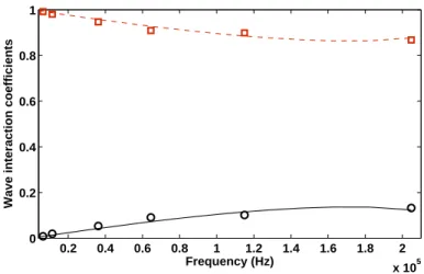
0.2 0.4 0.6 0.8 1 1.2 1.4 1.6 1.8 2

x 105 0

0.2 0.4 0.6 0.8 1

Frequency (Hz)

Wave interaction coefficients

Figure 9: Absolute values of the wave reflection and transmission coefficients for the pressure propagating wave at harmonic frequency 3ωfor a

nonlinearly hardened element with knl=1e13N/m3: Reflection coefficients computed according to the current scheme (–), Reflection coefficients

computed through a full transient FE calculation (◦), Transmission coefficients computed according to the current scheme (-,), Transmission

coefficients computed through a full transient FE calculation ().

Figure 10: Schematic representation of the two healthy and elastic composite multilayer waveguides (a) and (b) coupled through an element (c)

exhibiting structural nonlinearity.

In practice, the wave modes can be excited one-by-one in a full FE transient simulation by employing the WFE

computedφ+_q,n eigenvectors and applying them as time-dependent harmonic displacement boundary conditions (of excitation frequencyω) at one of the extreme cross-sections of the waveguide. An 11-cycle Hanning window was

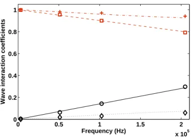
used for all transient excitations. The results on the fundamental and harmonic reflections for a nonlinearly

hard-ening element are presented below in Figs.11. Excellent agreement is observed between the fundamental frequency

reflection predictions obtained through the presented approach and through a full FE transient response prediction.

Moreover, good agreement is observed between the two approaches regarding the reflections computed for the 3ω

harmonic frequency. The most probable cause of the slight divergence observed between the two sets of results is the

fact that in a nonlinear transient FE problem energy is partially also channeled towards other harmonics (other than

the second one), which are not included in the harmonic balance expansion.

4. Conclusions

A novel comprehensive FE-based computational scheme was presented for quantifying guided wave interaction

with LSNs. Layered complex structures can be modelled through the presented approach as an FE discretization is

0 0.5 1 1.5 2

x 105 0

0.2 0.4 0.6 0.8 1

Frequency (Hz)

Wave interaction coefficients

Figure 11: Absolute values of the wave reflection and transmission coefficients of the pressure propagating wave for a nonlinearly hardened element

with knl=1e13N/m3at: Reflection coefficients at frequencyωcomputed according to the current scheme (–), Reflection coefficients at frequency

ωcomputed through a full transient FE calculation (◦), Reflection coefficients at frequency 3ωcomputed according to the current scheme (· · ·),

Reflection coefficients at frequency 3ωcomputed through a full transient FE calculation (⋄), Transmission coefficients at frequencyωcomputed

according to the current scheme (-,), Transmission coefficients at frequencyωcomputed through a full transient FE calculation (), Transmission

coefficients at frequency 3ωcomputed according to the current scheme (-·-), Transmission coefficients at frequency 3ωcomputed through a full

transient FE calculation (+).

employed. The scheme couples wave propagation properties within linear structural waveguides to LSNs and is able

to compute the generation of harmonic frequencies for each wave mode through a harmonic balance projection. The

principal outcomes of the work are summarized as follows:

(i) The presented scheme was validated through comparison with a full FE transient response prediction. Excellent

agreement is observed between the two sets of results for the fundamental, as well as for higher harmonic frequency

predictions.

(ii) The new approach is able to predict reflections and transmissions at harmonic frequencies with a speed that is

orders of magnitude faster than conventional transient FE solutions. The exhibited approach focuses on calculations

for 1D structures with a 2D methodology extension currently under development.

(iii) Generation of higher order harmonics can become maximum at certain frequencies which can be excited for

facilitating the detection of certain nonlinearity scenarios (ideally related to the presence of certain damage).

Future developments are focusing towards modelling and implementing realistic damage models as a LSN.

Ef-ficient multiscale damage models are essential to develop in order to accurately capture the nonlinear mechanics of

advanced damage scenarios, while retaining the size of the FE model and the implied required computational effort at

References

[1] C. Lissenden, Y. Liu, J. Rose, Use of non-linear ultrasonic guided waves for early damage detection, Insight-Non-Destructive Testing and

Condition Monitoring 57 (2015) 206–11.

[2] S. S. Kessler, S. M. Spearing, C. Soutis, Damage detection in composite materials using lamb wave methods, Smart Materials and Structures

11 (2002) 269.

[3] M. Breazeale, D. Thompson, Finite-amplitude ultrasonic waves in aluminum, Applied Physics Letters 3 (1963) 77–8.

[4] A. Vakakis, Scattering of structural waves by nonlinear elastic joints, Journal of vibration and acoustics 115 (1993) 403–10.

[5] A. H. Nayfeh, A. F. Vakakis, T. A. Nayfeh, A method for analyzing the interaction of nondispersive structural waves and nonlinear joints,

The Journal of the Acoustical Society of America 93 (1993) 849–56.

[6] P. B. Nagy, Fatigue damage assessment by nonlinear ultrasonic materials characterization, Ultrasonics 36 (1998) 375–81.

[7] D. M. Donskoy, A. M. Sutin, Vibro-acoustic modulation nondestructive evaluation technique, Journal of intelligent material systems and

structures 9 (1998) 765–71.

[8] V. Zaitsev, V. Nazarov, V. Gusev, B. Castagnede, Novel nonlinear-modulation acoustic technique for crack detection, NDT & E International

39 (2006) 184–94.

[9] V. J. Rao, E. Kannan, R. V. Prakash, K. Balasubramaniam, Fatigue damage characterization using surface acoustic wave nonlinearity in

aluminum alloy aa7175-t7351, Journal of Applied Physics 104 (2008) 123508.

[10] H. Hu, W. Staszewski, N. Hu, R. Jenal, G. Qin, Crack detection using nonlinear acoustics and piezoceramic transducersinstantaneous

amplitude and frequency analysis, Smart Materials and Structures 19 (2010) 065017.

[11] Z. Su, C. Zhou, M. Hong, L. Cheng, Q. Wang, X. Qing, Acousto-ultrasonics-based fatigue damage characterization: Linear versus nonlinear

signal features, Mechanical Systems and Signal Processing 45 (2014) 225–39.

[12] H. J. Lim, H. Sohn, M. P. DeSimio, K. Brown, Reference-free fatigue crack detection using nonlinear ultrasonic modulation under various

temperature and loading conditions, Mechanical Systems and Signal Processing 45 (2014) 468–78.

[13] K.-A. Van Den Abeele, P. A. Johnson, A. Sutin, Nonlinear elastic wave spectroscopy (news) techniques to discern material damage, part i:

nonlinear wave modulation spectroscopy (nwms), Research in nondestructive evaluation 12 (2000) 17–30.

[14] K. E. Van Den Abeele, A. Sutin, J. Carmeliet, P. A. Johnson, Micro-damage diagnostics using nonlinear elastic wave spectroscopy (news),

Ndt & E International 34 (2001) 239–48.

[15] M. Meo, U. Polimeno, G. Zumpano, Detecting damage in composite material using nonlinear elastic wave spectroscopy methods, Applied

composite materials 15 (2008) 115–26.

[16] M. Scalerandi, V. Agostini, P. P. Delsanto, K. Van Den Abeele, P. A. Johnson, Local interaction simulation approach to modelling nonclassical,

nonlinear elastic behavior in solids, The Journal of the Acoustical Society of America 113 (2003) 3049–59.

[17] P. P. Delsanto, A. Gliozzi, M. Hirsekorn, M. Nobili, A 2d spring model for the simulation of ultrasonic wave propagation in nonlinear

hysteretic media, Ultrasonics 44 (2006) 279–86.

[18] C. Pecorari, Nonlinear interaction of plane ultrasonic waves with an interface between rough surfaces in contact, The Journal of the Acoustical

Society of America 113 (2003) 3065–72.

[19] A. J. Croxford, P. D. Wilcox, B. W. Drinkwater, P. B. Nagy, The use of non-collinear mixing for nonlinear ultrasonic detection of plasticity

and fatigue, The Journal of the Acoustical Society of America 126 (2009) EL117–22.

[20] V. Giurgiutiu, M. Gresil, B. Lin, A. Cuc, Y. Shen, C. Roman, Predictive modeling of piezoelectric wafer active sensors interaction with

high-frequency structural waves and vibration, Acta Mechanica 223 (2012) 1681–91.

[21] Y. Shen, V. Giurgiutiu, Predictive modeling of nonlinear wave propagation for structural health monitoring with piezoelectric wafer active

sensors, Journal of Intelligent Material Systems and Structures 25 (2014) 506–20.

[22] T. B. Autrusson, K. G. Sabra, M. J. Leamy, Reflection of compressional and rayleigh waves on the edges of an elastic plate with quadratic

nonlinearity, The Journal of the Acoustical Society of America 131 (2012) 1928–37.

[23] G. M. Fierro, F. Ciampa, D. Ginzburg, E. Onder, M. Meo, Nonlinear ultrasound modelling and validation of fatigue damage, Journal of

Sound and Vibration 343 (2015) 121–30.

[24] N. Rauter, R. Lammering, T. K ¨uhnrich, On the detection of fatigue damage in composites by use of second harmonic guided waves,

Composite Structures 152 (2016) 247–58.

[25] K.-Y. Jhang, Nonlinear ultrasonic techniques for nondestructive assessment of micro damage in material: a review, International journal of

precision engineering and manufacturing 10 (2009) 123–35.

[26] I. Solodov, D. D ¨oring, G. Busse, New opportunities for ndt using non-linear interaction of elastic waves with defects, Strojniˇski

vestnik-Journal of Mechanical Engineering 57 (2011) 169–82.

[27] K. Matlack, J.-Y. Kim, L. Jacobs, J. Qu, Review of second harmonic generation measurement techniques for material state determination in

metals, Journal of Nondestructive Evaluation 34 (2015) 1–23.

[28] D. Broda, W. Staszewski, A. Martowicz, T. Uhl, V. Silberschmidt, Modelling of nonlinear crack–wave interactions for damage detection

based on ultrasounda review, Journal of Sound and Vibration 333 (2014) 1097–118.

[29] D. Mead, A general theory of harmonic wave propagation in linear periodic systems with multiple coupling, Journal of Sound and Vibration

27 (1973) 235–60.

[30] R. Langley, A note on the force boundary conditions for two-dimensional periodic structures with corner freedoms, Journal of Sound and

Vibration 167 (1993) 377–81.

[31] B. R. Mace, D. Duhamel, M. J. Brennan, L. Hinke, Finite element prediction of wave motion in structural waveguides, The Journal of the

Acoustical Society of America 117 (2005) 2835–43.

[32] D. Duhamel, B. R. Mace, M. J. Brennan, Finite element analysis of the vibrations of waveguides and periodic structures, Journal of Sound

and Vibration 294 (2006) 205–20.

[33] J. M. Renno, B. R. Mace, On the forced response of waveguides using the wave and finite element method, Journal of Sound and Vibration

329 (2010) 5474–88.

[34] D. Chronopoulos, M. Ichchou, B. Troclet, O. Bareille, Computing the broadband vibroacoustic response of arbitrarily thick layered panels

by a wave finite element approach, Applied Acoustics 77 (2014) 89–98.

[35] D. Chronopoulos, B. Troclet, O. Bareille, M. Ichchou, Modeling the response of composite panels by a dynamic stiffness approach, Composite

Structures 96 (2013) 111–20.

[36] D. Chronopoulos, M. Ichchou, B. Troclet, O. Bareille, Predicting the broadband response of a layered cone-cylinder-cone shell, Composite

Structures 107 (2014) 149–59.

[37] J.-M. Mencik, M. Ichchou, Multi-mode propagation and diffusion in structures through finite elements, European Journal of

Mechanics-A/Solids 24 (2005) 877–98.

[38] J. M. Renno, B. R. Mace, Calculation of reflection and transmission coefficients of joints using a hybrid finite element/wave and finite element

approach, Journal of Sound and Vibration 332 (2013) 2149–64.

[39] R. Langley, K. Heron, Elastic wave transmission through plate/beam junctions, Journal of sound and vibration 143 (1990) 241–53.

[40] R. E. Mickens, Truly nonlinear oscillations: harmonic balance, parameter expansions, iteration, and averaging methods, World Scientific,

2010.

[41] R. K. Narisetti, M. Ruzzene, M. J. Leamy, Study of wave propagation in strongly nonlinear periodic lattices using a harmonic balance

approach, Wave Motion 49 (2012) 394–410.

[42] F. Moser, L. J. Jacobs, J. Qu, Modeling elastic wave propagation in waveguides with the finite element method, NDT & E International 32

(1999) 225–34.

[43] K. Manktelow, R. K. Narisetti, M. J. Leamy, M. Ruzzene, Finite-element based perturbation analysis of wave propagation in nonlinear