Image processing in echography and MRI

University of Southampton Research Repository

ePrints Soton

Copyright © and Moral Rights for this thesis are retained by the author and/or other

copyright owners. A copy can be downloaded for personal non-commercial

research or study, without prior permission or charge. This thesis cannot be

reproduced or quoted extensively from without first obtaining permission in writing

from the copyright holder/s. The content must not be changed in any way or sold

commercially in any format or medium without the formal permission of the

copyright holders.

When referring to this work, full bibliographic details including the author, title,

awarding institution and date of the thesis must be given e.g.

AUTHOR (year of submission) "Full thesis title", University of Southampton, name

of the University School or Department, PhD Thesis, pagination

UNIVERSITY OF SOUTHAMPTON

. . .

Image Processing in Echography and

MRI

by

Bernardo S. Carmo

A thesis submitted in partial fulfillment for the

degree of Doctor of Philosophy

in the

Faculty of Engineering, Science and Mathematics

School of Electronics and Computer Science

UNIVERSITY OF SOUTHAMPTON

ABSTRACT

FACULTY OF ENGINEERING, SCIENCE AND MATHEMATICS SCHOOL OF ELECTRONICS AND COMPUTER SCIENCE

Doctor of Philosophy

by Bernardo S. Carmo

This work deals with image processing for three medical imaging applications: speckle detection in 3D ultrasound, left ventricle detection in cardiac magnetic resonance imag-ing (MRI) and flow feature visualisation in velocity MRI.

Contents

Acknowledgements

1 Introduction

1.1 Medical Imaging 1.2 Thesis Outline .

2 Speckle Detection for 3D Ultrasound 2.1 Theory of Speckle. . . .

2.1.1 Speckle Detection . . . . 2.2 Classifier Implementation and Assessment 2.3 Discussion... 3 Cardiac MRI Acquisition and Display

3.1 Cardiac blood flow . . . . 3.2 Cardiac MRI acquisition . . . . 3.3 Other Clinical Assessment Techniques 3.4 MRI Flow Visualisation

3.4.1 Streamline Plots 3.4.2 Field Topology .

4 Left Ventricle Detection with Template Matching 4.1 Previous work on medical image segmentation. 4.2 Detection algorithm design

4.2.1 System requirements 4.2.2 Template matching. 4.2.3 Hough transform 4.3 Test results

4.4 Discussion...

5 Vector Field Restoration for Blood Flow MRI 5.1 Restoration algorithm . . . .

5.2 Related Work . . . . 5.2.1 Simple Gaussian Smoothing. 5.2.2 Anisotropic Smoothing. 5.3 Materials and Methods . . .

5.3.1 Flow Field Restoration. 5.4 Results and Discussion.

5.5 Conclusions...

CONTENTS

6 Visualisation of Three-Dimensional Velocity MRI 6.1 Introduction . . . . 6.2 Previous Work . . . .

6.2.1 Occurrence of Vortical Flow in the Cardiac Cycle. 6.2.2 Vector Field Visualisation

6.2.3 Data Clustering. . . . 6.3 Materials and Methods. . . . 6.3.1 Clustering Implementation 6.3.2

6.3.3

Local Linear Expansion . . Topology Display . . . .

m

81 81

82

82

96

99

99

6.4 Results... . 105

6.5 Discussion . . . . 7 Conclusions and Future Work

7.1 Segmentation for 3D Ultrasound 7.2 Segmentation for Cardiac MRI . 7.3 Noise Reduction of 3D Velocity MRI 7.4 Feature Abstraction for 3D Velocity MRI 7.5 Preliminary Approaches for Further Work Bibliography

.106

111 .111 .112 .113 .113 .114

Acknowledgements

I would like to thank my supervisor, Dr. Adam Priigel-Bennett. This work was sup-ported by Portuguese FCT grant BD /1318 and a UK EPSRC grant. Additional guidance by Dr. Andrew Gee and Dr. Richard Prager, University of Cambridge, and by Prof. G.

z.

Chapter

1

Introduction

A considerable amount of knowledge about human anatomy has been accumulated throughout the centuries through the application of invasive methods. Today, this type of procedure still has to be performed on patients for diagnostic purposes, for example biopsies to determine the malignancy of a tumour, or open-brain surgical attachment of electrodes for locating sources of epileptic seizures. Research is underway to replace these and other methods with non-invasive techniques, which do not require direct access to the body's interior.

1.1

Medical Imaging

Medical imaging consists of a set of technologies that enable physicians to "see" inside the human body [40, 7J. Current imaging modalities used in clinical practice include X-ray films and computerised tomography (CT), radioisotope imaging, magnetic resonance imaging (MRI) including velocity MRI and functional MRI, single-photon emission to-mography (SPECT), magnetic source imaging, surface light scanning and ultrasound (US), including two-dimensional frames from array probes (B-scans) and intra-vascular probes (JVUS) [262J. General 3D medical imaging has been researched since the 1970s and used clinically for about 15 years [242J. Historically, the first applications of 3D med-ical imaging consisted of imaging bones in CT, soft-tissue in MRI, and interventional and surgery assistance. The objects of interest in 3D medical imaging may be rigid (e.g., bones), deformable (e.g., soft-tissue structures), static (e.g., skull), or dynamic (e.g. heart, joints). In many applications, the analysis may focus on several objects. For example, an MRI 3D study of a patient's head may focus on three 3D objects: the white matter, the gray matter, and the cerebrospinal fluid. The information sought via 3D medical imaging may be qualitative or quantitative in nature. In qualitative analy-sis, mostly visual data is required, and the predominant issues are how to extract and display such information for human visualisation. In quantitative studies, we seek to

Chapter 1 Introduction 2

measure or estimate parameters about the objects' morphology or function. In many applications, extensive user involvement is required, for example in the form of manual delineation of organ contours in tomographic images.

3D medical image processing and analysis systems generally consist of the following modules: a) pre-processing, including restricting the volume of interest for efficient data storage, filtering to supress or enhance information, interpolation to modify the level of discretisation, registration to combine information from multiple sources or viewpoints, and segmentation to assign image points to anatomic features; b) visualisation, which can be slice-based if the given scene is broken up into 2D slices that are displayed, or volume-based if the 3D object information in the scene is directly rendered using various techniques; c) manipulation, used to simulate surgery procedures and to develop aids for therapy procedures, and include operations to cut, separate, move, mirror, stretch, compress and bend objects; d) analysis, which aims to quantify morphological/functional information about the objects in the scene, yielding data such as density measures, intensity statistics, velocity, distance, length, curvature, area volume and mechanical properties.

This thesis deals with the first stage, pre-processing of medical image data. It addresses segmentation, noise reduction and feature detection, and makes a contribution towards resolving some of the current issues in those areas. This facilitates subsequent processing. Visualisation is improved by noise reduction, as the displayed data contains more of the desired information. Noise reduction also improves the accuracy of analysis, as clinical measures are not misled by random signal fluctuations. Segmentation brings direct benefits to visualisation, as rendering can then display only segmented image sections of interest. This is, of course, possible with manual segmentation. However, fully or even semi-automatic segmentation generally result in significant time savings in reduced operator time. The benefits of this are obvious in a clinical setting, when required to handle hundreds of patients. For manipulation, a noise-reduced or segmented dataset is usually easier to manipulate than raw data, because considerable data reduction has taken place. If the manipulation is operator-driven, the improved rendering of segmented data makes the manipulation task easier and more intuitive. For analysis, segmented data can be analysed quicker or even immediately. Organ volumes from 3D scans, for example, are trivial to measure if the organs in question have already been segmented. Another application is the measurement of mechanical properties of the heart, which can be computed directly from a segmented dataset.

Chapter 1 Introduction 3

and ejection fraction. The Dutch company Medis has a range of products for Echogra-phy and MRI, starting from full direct visualisation of raw data to cardiovascular flow velocity analysis and semi-automated angiography. Stradx (Department of Engineer-ing, Cambridge University) is an acquisition and analysis program for 3D Echography, containing facilities for any-plane reslicing, semi-automated segmentation, volume ren-dering and volume measurement. Medical scanner manufacturers also provide a set of software applications to be used in conjunction with the scanner. The facilities provided are generally basic but certified to be reliable for daily medical use.

Segmentation, in particular, continues to be a bottleneck in clinical analysis packages. Much operator time is still spent on manual delineation of organ or vessel contours, for further processing, because fully available automatic systems are still an area of research. In many applications of 3D ultrasound, a volume of interest must be found before rendering due to noise and occlusion, and in order to compute measurements within that volume. In 3D cardiac MRI, there is less of a visualisation requirement and more of analysis: the left ventricle must be found, in order for elasticity, extensibility and other vital measures to be taken. In 3D velocity MRI, a method of acquiring blood flow information inside the human heart and vessels, direct visualisation of the flow patterns is impossible without automatic flow analysis, because of the large size of the dataset, and occlusion by other image features. In time series acquisitions, there is an added tracking challenge since the structures of interest move with time. In order for analysis to be carried out, those features must be tracked reliably to ensure that the measurements are being taken consistently over the same flow feature. This is further complicated when features end and new ones appear, or when the borders between them are unclear. The tracking aspect of time series acquisitions is not addressed in this thesis.

1.2 Thesis Outline

Cbapter 1 Introduction 4

principle, a reliable means of finding speckle in the image is necessary. An asessment of existing methods, and the proposal and assessment of a novel method, are presented in chapter 2.

Essential background theory is introduced in chapter 3 on the Magnetic Resonance Imag-ing (MRI) modality and its flow variant, Velocity MRI. This is in preparation for the following three chapters, which deal with our research on these modalities. Chapter 4 deals with the detection of the left ventricle in cardiac MRI. This acquision mode cap-tures MRI slices of the heart at different phases of the cardiac cycle and can generate image frame sequences or even movies. More clinically relevant for the study of pathol-ogy, however, is the quatitative evaluation of flow and mechanical characteristics related to the mechanical pumping function of the heart. There are several relevant measures associated with the movement of the left ventricle, but at present the extraction of these measures suffers from the important bottleneck of segmentation of the ventricle borders. Extensive manual intervention by a qualified techician is required to pinpoint the loca-tion of the left ventricle in each frame for each new patient. We assess the current state of automation software in this field and present our findings in the study of an original template-based method.

Chapter 5 describes our work on the first step of a three-step framework for processing cardiac blood flow Velocity MRI data. The framework consists of restoration of the noise-corrupted flow field, abstraction to extract relevant features, and tracking to find correspondences between features in different time frames. The first step has been fully implemented using total variation and the first-order method, and its effectiveness assessed. Results are presented for its application to simulated 3D flow data, including simulated flow of blood inside the heart. The method was first successfully applied to 2D in vivo data by a different author (see [175, 176]).

The abstraction step deals primarily with the detection of vortices in the blood flow inside the heart, and is closely related to the clinical study of cardiac function following infarction, or heart attack. At the onset of disease, a vortex ring can be observed in the cardiac flow which increases in size and vorticity with the passing weeks, primarily a result of an enlarged left ventricle. It is important to detect this vortex ring and analyse its characteristics in patients, for diagnostic and also for research purposes. This presents a main problem for visualisation: flow surrounding the vortices will occlude these from the observer. Chapter 6, presents our solution to this which combines clustering, local linear expansion and automatic streamline selection.

Papers published

Chapter 1 Introduction 5

Ng, Y. H. P., Carmo, B. S., Priigel-Bennett, A. and Yang, G. Z. A first order Lagrangian based variational approach for MR flow vector field restoration. Proc. Computer As-sisted Radiology and Surgery (CARS) 2003.

Ng, Y. H. P., Carmo, B. S. and Yang, G. Z. Flow Field Abstraction and Vortex Detection For MR Velocity Mapping. Proc. MICCAI 2003, Lecture Notes in Computer Science 2878:424-431.

Chapter 2

Speckle Detection for 3D

Ultrasound

In this section we describe our work and experiments involving a fully automatic segmen-tation method: a pattern classifier for detecting speckle in ultrasound images. Speckle detection is required for sensor-less recording of ultrasound (US) probe position through speckle decorrelation.

As we referred earlier, freehand 3-D ultrasound employs a procedure whereby the clin-ician is allowed to move the probe as in a normal B-mode examination. The probe's position is tracked by the system's hardware, which allows its software to position frames relative to each other in order to produce a 3-D dataset. Determination of probe move-ment can be achieved by several methods, including magnetic and optical position sen-sors. In both cases, a position beacon is attached to the handheld probe while a fixed detector assembly determines the beacon's placement in 3-D space. With appropriate calibration, the 3-D ultrasound system is able to label each B-scan with the position and orientation of the scan plane. Currently available positioning systems are expensive and complicated to install and use. They also have limited accuracy, which makes it highly desirable to replace them with more sensitive techniques, or otherwise to com-plement them with other sources of position data. Such an enhancement could increase the accuracy of organ and tumour volume measurement using freehand 3-D ultrasound, and also enable better 3-D reconstruction of images produced by the more recent high-definition ultrasound probes. According to current research, this may be achieved using information present in the images themselves, using speckle decorrelation [37, 225, 240]. Ultrasound images contain several types of features: anatomically-related structures, which result from the interaction between the ultrasound waves and tissue structures and boundaries; artifacts and noise, which are caused by hardware and software lim-itations and do not express any actually existing structures; and speckle, a globular

Chapter 2 Speckle Detection for 3D Ultrasound 7

FIGURE 2.1: An ultrasound speckle pattern.

pattern generally found in areas of the image which correspond to homogeneous tissue (Figure 2.1).

Ultrasound speckle is an image structure that does not correspond to any existing

struc-ture in the tissue being imaged. In fact, because the tissue is homogeneous, a uniform brightness level would be expected to appear in the corresponding area of the image.

In-stead, a pattern is displayed. This pattern has been found to be determined by physical

characteristics of the ultrasound transducer being used, as well as scattering properties of the insonified tissue volume.

If the ultrasound probe is held stationary during a scan, the pattern of speckle remains

unchanged if the subject is stilll. Two successive, closely-spaced B-scan frames of a

freehand probe sweep contain areas of speckle with measureable correlation. The level of decorrelation which results from moving the probe in the elevational (out-of-plane) direction can be used to determine the extent of the displacement. Therefore, given the

precise location of speckle areas in the image, and their correspondence in successive frames, it is possible to determine their level of decorrelation in order to calculate probe movement.

Speckle tracking and decorrelation methods have the potential to enhance performance

or even eliminate the need for a separate position sensor, because they can provide

the ultrasound system with position and orientation information gathered from data

present in the B-scan frames alone. Commercially available systems that have replaced external position sensors employ proprietary techniques that involve some form of speckle

decorrelation, combined with other methods such as Doppler spectra and echo timing

using multiple-line probes [38, 81, 265, 266].

Chapter 2 Speckle Detection for 3D Ultrasound 8

In the next sections we present the theory of ultrasound speckle and its relationship with the optical theory of laser speckle. We also explain its relevance towards current research in speckle detection and classification for tissue identification. We then report on our own studies for detecting and tracking speckle regions, and we compare our results with previous techniques.

2.1

Theory of Speckle

Speckle appears in ultrasound images as a characteristic granular pattern, generally in areas corresponding to homogeneous tissue. The expected representation would be a uniform brightness level, but random-looking signal fluctuations appear instead. Because the actual tissue being imaged does not contain any structures resembling the granular pattern, speckle is usually classified as a B-scan artifact. It is sometimes an undesired feature, since it inhibits detection of low-contrast structures [5, 48, 99].

The cause of speckle is believed to be scattering by reflectors smaller than the resolution cell (the smallest region that can be resolved by the ultrasound beam). These reflectors are called non-specular; tissue boundaries, which are represented in B-scans by sharp lines, are called specular reflectors. At each non-specular reflector, a scattered wave front is emitted in all directions. Multiple wave fronts from the all the scatterers in each resolution cell reach the transducer with various phases, which results in the well-known phenomenon of interference (Figure 2.2). Because of the very small magnitudes involved, the combined contribution is unpredictable and must be treated statistically. Speckle patterns are not random in the same sense as, for example, electrical noise, which is also present in B-scans. When an object is scanned twice in the same position under the same conditions, the resulting B-scans contain identical speckle patterns. Furthermore, the size of the speckle granules is approximately the same as the lateral and axial resolution of the scanner [28].

At present there are no well-defined criteria in the literature for systematically locat-ing speckle in an ultrasound image - it is not possible to state with certainty whether a selected image region contains features which are attributable exclusively to speckle phenomena. What is known, however, is that speckle arises in image regions that corre-spond to parenchymal tissue2, or any other medium which is homogeneous throughout

(e.g. blood, placenta) and contains a critical concentration of sub-resolution particles called scatterers. Besides speckle, the image may also be corrupted by random hardware noise and acoustic artifacts. As we will see in the next section, many speckle detection algorithms are based on knowledge of the process of speckle formation, from which a characteristic signature is derived and used as a search criterion.

Chapter 2 Speckle Detection for 3D Ultrasound 9

,---,--+----

-

-'

Transducer

~~---­

~

---T

-

Non-specular reflectors

FIGURE 2.2: Production of a speckle pattern. Each non-specular reflector, smaller than the resolution cell, receives the ultrasound pulse and produces a scattered wave-front in all directions. The wavewave-fronts from all the reflectors in the cell return to the ultrasound transducer as echoes with various phases, causing interference. This phe-nomenon occurs at resolution cells that contain a critical number of scatteres, which

results in a speckle pattern being formed in the ultrasound B-scan image frame.

In optics, a phenomenon similar to speckle occurs when a beam of coherent light (such as a laser) strikes a rough surface and is reflected back: the roughness of the surface causes multiple reflections to reach the detector and interfere with each other. This adding up of many sinusoidal pulses with statistically independent phases leads to the random walk phenomenon. For the purposes of speckle signature prediction in B-scans, the current theory on speckle adopts a model that is analogous to the optical counterpart.

Treating the echo signal amplitudes throughout the B-scan frame as a stochastic vari-able, the statistics of its distribution can be predicted theoretically. The echo signal is modelled as a sum of components in the complex plane. Each component is the contri-bution of an individual scatterer in a resolution cell. The complex echo signal returned from that cell is stochastic and can be shown to obey a complex Gaussian probability density function (PDF) if the number of scatterers is large [90J. Processing removes the phase component by envelope detection, and the processed signal can be shown to follow a Rayleigh amplitude PDF. If a coherent background is added, a constant strong component arises which transforms this into a Rician PDF, of which the Rayleigh PDF is a special case [258J. The more general K distribution describes the scatterer densities below the critical limit. These PDFs are termed first-order statistics because they deal with the intensity of each point in the image.

Chapter 2 Speckle Detection for 3D Ultrasound

10

of trying to predict the PDF of the post-processed signal, the original data can be reconstructed approximately [125] and corrected to compensate for non-linear mappings introduced by the equipment [191].

In the next section, we discuss the consequences of the random walk model, and report on its applications for the purpose of detecting speckle in B-scan image frames.

2.1.1

Speckle Detection

Automatic recognition of speckle patterns in B-scan image frames may employ two types of algorithms: speckle-specific, where the statistics of signal distribution are predicted theoretically from the model of speckle formation and used as a signature for speckle detection and classification; and generalised image processing methods that quantify the distribution of brightness levels and build a texture library, from which classes are derived for image region segmentation.

Speckle detection has important applications in image noise reduction, tissue characteri-sation for diagnosis, blood flow measurement, automatic image segmentation for volume measurement and, as mentioned before, probe movement detection in 3-D ultrasound when combined with speckle decorrelation. In this section, we survey previous and cur-rent research in this area and discuss possible applications. We also present results from our own studies.

Signal-to-Noise Ratio

The fractional n-order signal-to-noise ratio (SNR) of a signal Xi with N samples is defined [68] as:

where

and

A(n)

SNR(n)=-s(n)

s(n) = _1_

~(X?l

A~n))2

N-IL..t t t

i=l

(2.1)

(2.2)

(2.3)

Chapter 2 Speckle Detection for 3D Ultrasound 11

Autocorrelation Function

The autocorrelation function (ACF) is a popular second order texture statistic. It is defined [226J as:

'\;'M -p '\;'N -q I( . ')1(' . ) ACF _ MN L....i=l L....j=l ~,] ~ + P,] + q

(p, q) - (M - p)(N - q)

2:f'!1 2:f=1 J2(i,j)

where p,q is the position difference in the i,j direction, and M,N are the image I's dimensions. The ACF measures the area integral of the internal (dot) product between an image region and its copy, displaced by a varying distance along a chosen direction. The integral is evaluated only where the two patches overlap, and is normalised by the area of overlap [97J.

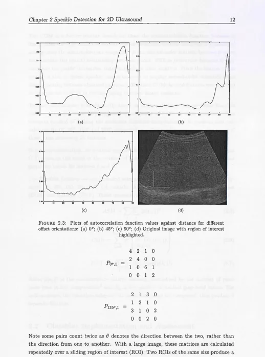
Wagner et al. [257J evaluated this integral as distance is increased, using patches of simulated Rician speckle. Beyond a certain distance, their plot resembles a sinusoid-shaped curve whose Fourier transform can be fitted well by a Gaussian. This is to be expected since single frequency structured speckle was used. This type of speckle does not exist in real images, which in our view explains why the paper's strategy of classifying speckle by measuring peak differences in the ACF plot was unsuccessful. In our own experiments, we produced ACF plots for p,q varying along 0°,45° and 90°. We found that peaks and valleys could appear at various, unpredictable positions in the sequence, in agreement with [3J. The plots in Figure 2.3 are typical of the problem. This irregularity makes the technique of measuring peak value and position differences meaningless for the purposes of ACF curve classification of in vivo US display images. This problem may be alleviated when the unmodified intensity data is available as in Wagner et al [257], but that is not the case in our study.

Co-occurrence Matrix

The co-occurrence matrix COMo,d(a, b) measures how frequently two image pixels with grey levels a, b appear separated by a distance d along direction

e

0 0 1 1 0 0 1 1 0 2 2 2 2 2 3 3

Chapter 2 Speckle Detection for 3D Ultrasound

1.03 I.'

1.02

1.3 1.01

12

1.1

0.'"

0.95

0 \0 20

(a) (b)

1.011

1.06 1.04 1.02

0.96

O.940!-~\o---:2~0 --=30--40~----=:50:---::---::7!):---::----:!.

(c) (d)

FIGURE 2.3: Plots of autocorrelation function values against distance for different offset orientations: (a) 00; (b) 450; (c) 900; (d) Original image with region of interest

highlighted.

4 2 1 0

2 4 0 0

Poo ,l

1 0 6 1

0 0 1 2

2 1 3 0

Pl35o,l

1 2 1 0

3 1 0 2

0 0 2 0

12

Note some pairs count twice as

e

the direction from one to another. With a large image, these matrices are calculated

repeatedly over a sliding region of interest (ROI). Two ROls of the same size produce a

Chapter 2 Speckle Detection for 3D Ultrasound 13

The COM is a better texture descriptor than the autocorrelation function because it distiguishes the information at various spatial distances, whereas the latter is a measured average over the entrire distance range [96]. It is a second-order statistic because it takes into account the spatial relationship between pixels. SNR is first-order because it only considers the pixels' intensities, independently of their location. Since the human vision system is able to detect speckle, and is believed to employ second-order statistics when discriminating between observed patterns [122], then COM-derived features are expected to be superior to SNR in distinguishing between image patterns.

Texture classification is traditionally based on criteria derived from so-called Haralick features. Haralick et al. [97] suggested 14 measures and defined their equations. The common method of making the measures direction-independent is to perform four cal-culations for 00

, 90 0

, 180 0

and 2700

respectively, and computing the mean and range of these, thus obtaining 24 features.

In our implementation, we grouped grey levels in intervals of 10, so for example element (1,1) contains the count of the number of pairs of pixels separated by d along

e

The Haralick features we implemented were the ones most frequently used in the liter-ature [25, 255, 155, 282, 245, 12], namely: Angular Second Moment (ASM), Contrast (CON) and Entropy (ENT). These measures are defined as follows:

ASM =

'L'L

ENT = -

'L

(2.5)

(2.6)

(2.7)

where p(i,j) is the co-occurrence matrix element, normalised by the number of pixel pairs used in the computation3 and Ng is the number of distinct grey-level values. For each measure, the direction-independent mean and range are computed, thus yielding 6 separate features.

2.2

Classifier Implementation and Assessment

Chapter 2 Speckle Detection for 3D Ultrasound 14

performance of several image feature extraction mechanisms in detecting speckle. In the second phase, results from this assessment were combined to devise a combined speckle detection strategy.

Learning From Data Approach

SNR and COM are examples of image features - they are measures that enable the assignment of image pixels to classes. In the present study, there are two classes: the regions in the ultrasound image that contain speckle, and those that don't.

We assume that each class is defined by decision boundaries, which are upper and lower thresholds of feature values. Pixels with feature values lying inside this range belong to the class, otherwise they belong to a different class.

In practice, classes have feature ranges that overlap, and the choice of decision boundaries is approximate and introduces error. The average probability of classification error P(error} is defined as the probability of assigning each pixel to the wrong class, based on the chosen decision boundaries.

Here, we locate decision boundaries by searching in feature space for the thresholds that yield the lowest P (error). This is defined as:

P( ) _ no. of missed pixels

+

error - . .

Image sIze (2.8)

Missed pixels are speckle pixels classified as non-speckle, and misclassified pixels are non-speckle pixels classified as speckle.

The optimal range of feature values is computed by running this search over a set of images called the training set. The average P{error} obtained gives an indication of the best-case error to be expected, but not necessarily achieved, in practice. A realistic estimate of P{error} was obtained by applying the optimal range over a different, larger set of images usually called the testing set [103].

Speckle Detection Assessmet

We implemented a pattern classifier that computes value ranges on several features from training images, and measures the resulting P{error} on test images.

Chapter 2 Speckle Detection for 3D Ultrasound 15

a qualified radiologist. Frames were divided in equal proportions between the training dataset (111 images) and the test dataset (222 images), yielding a total of 333 images. Speckle in these images was marked manually. A separate manual segmentation im-age was created by this author for each dataset imim-age. The manual segmentation also included pixels in the image that do not correspond to ultrasound information (image canvas) for correct P(error} determination. This process relied on the operator's expe-rience and knowledge of ultrasound image formation. The operator did not know which set each image belonged to (training or test), but he was aware of the algorithms under study.

For SNR, we implemented integral as well as fractional order moments taken from de-compressed data following the procedure in [191J (features SNR 0.25, SNR 0.5, SNR 0.75 and SNR 1.0 in Figure 2.4). Three estimates of the decompression parameter were computed for each Stradx dataset; this process, repeated for all Stradx datasets used in this study, yielded an estimate for the decompression parameter of 26.3 mean with a 7.1 standard deviation. The mean value was used to decompress all the images. The SNR for the given B-scan was also used (SNR I in Figure 2.4).

Training consisted of a search for a combination of three parameters that resulted in the lowest P(error} (computed by comparing the classifier output with the manual seg-mentation images). The parameters were the lower and upper thresholds of SNR value, and the size of the square sliding region of interest (ROI) used to compute the local SNR value. The search for thresholds was exhaustive over all values in the image; the search for the best ROI size was limited to widths between 24 and 84 pixels over 4-unit increments.

For COM, a search scheme identical to that for SNR was used, over the same range of ROI sizes. Each measure yielded a mean- and range-related feature ("m" and "r" in Figure 2.4).

The mean values of the lower and upper thresholds, and also of the square ROI sizes, obtained from training were used as fixed values to detect speckle using the same features over the test dataset. Manual segmentation images were only employed to measure the final error rates. For COM and SNR features, square ROI widths between 60 and 72 pixels were used.

The speckle detection algorithm (HOM) described in [191J was also assessed; since it requires no training, it was only run on the test dataset.

Chapter 2 Speckle Detection for 3D Ultrasound

0%

:E E E E .... LO 0 LO q _E ~

0 ~ Z I- 0:: N Ii) I'- _a.

::i!: z ₀ I- _{Z Z ci ci ci z U)}

:r:

~ U)

_«

() () W 0:: _Z 0:: _Z 0:: Z ( )

Z U)

U) U) U) ~

a. U) detection algorithm

FIGURE 2.4: Train and test results for all detection algorithms. Error bars were com-puted with the student-t test [161].

Discussion of performance results

16

Of the algorithms discussed here so far, all had training performances to within 5% of

each other. As for testing performance, COM-based algorithms performed best with

P{error) = 28%-31%, followed by SNR-based with 37%-38%, and HOM with 48%.

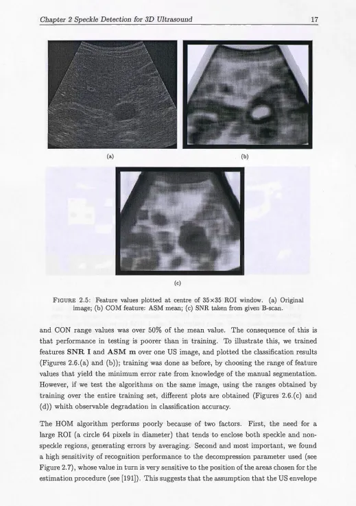
All COM features have a tendency to incorrectly mark noise as speckle. We can observe

from Figure 2.5 that shadow areas with a purely noisy pattern have feature values that

are very close to speckle zones. When setting optimal thresholds with COM features,

many noise regions are also marked. This may be acceptable for images with small patches of noise, but may produce large errors when the areas of noise are large. This

is particularly serious for e.g. pregnancy scans, with predominance of amniotic fluid

regions that generate large shadows.

We also found a noise-related issue when SNR measures are involved. Because of different

noise-reduction strategies employed by the US machine post-processor, shadow areas

may be displayed either as black regions if the filtering is strong, or as distinct noise if

the filtering is weak. This results in the SNR for such regions varying over a range which is unpredictable: black areas have a constant signal that has high SNR, whereas noise

areas have steep variations that reduce SNR. Different gain and timing settings on the machine may accentuate this issue.

Also, COM and SNR feature values vary over a large range for speckle areas alone. In

Chapter 2 Speckle Detection for 3D Ultrasound

(a) (b)

( c)

FIGURE 2.5: Feature values plotted at centre of 35x35 ROI window. (a) Original image; (b) COM feature: ASM mean; (c) SNR taken from given B-scan.

17

and CON range values was over 50% of the mean value. The consequence of this is

that performance in testing is poorer than in training. To illustrate this, we trained

features SNR I and ASM m over one US image, and plotted the classification results

(Figures 2.6.(a) and (b)); training was done as before, by choosing the range of feature

values that yield the minimum error rate from knowledge of the manual segmentation. However, if we test the algorithms on the same image, using the ranges obtained by

training over the entire training set, different plots are obtained (Figures 2.6.(c) and

(d)) whith observable degradation in classification accuracy.

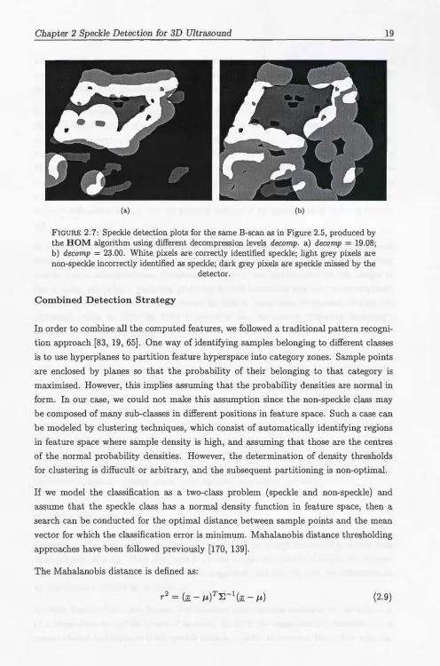
The HOM algorithm performs poorly because of two factors. First, the need for a

large ROI (a circle 64 pixels in diameter) that tends to enclose both speckle and

non-speckle regions, generating errors by averaging. Second and most important, we found

a high sensitivity of recognition performance to the decompression parameter used (see

Figure 2.7), whose value in turn is very sensitive to the position of the areas chosen for the

Chapter 2 Speckle Detection for 3D Ultrasound

(a) (b)

(c) (d)

FIGURE 2.6: Speckle detection plots for the same B-scan as in Figure 2.5. a) ASM m with optimal feature value range trained from manual segmentation data; b) SNR I,

also with trained feature value range; c) ASM m with range obtained from training over entire training set; d) SNR I, also from trained range. White pixels are correctly identified speckle; light grey pixels are non-speckle incorrectly identified as speckle; dark

grey pixels are speckle missed by the detector.

18

data may be reconstructed faithfully by simple exponentiation of the pixel values may

need to be revised. In fact, the handling of the RF echo data by the US machine, especially facilities for variable local gains and the rasterisation function, may modify

the data to an extent that makes actual image statistics differ highly from predicted

ones.

Chapter 2 Speckle Detection for 3D Ultrasound

(a) (b)

FIGURE 2.7: Speckle detection plots for the same B-scan as in Figure 2.5, produced by the HOM algorithm using different decompression levels decomp. a) decomp = 19.08; b) decomp = 23.00. White pixels are correctly identified speckle; light grey pixels are non-speckle incorrectly identified as speckle; dark grey pixels are speckle missed by the

detector.

Combined Detection Strategy

19

In order to combine all the computed features, we followed a traditional pattern

recogni-tion approach [83, 19, 65]. One way of identifying samples belonging to different classes

is to use hyperplanes to partition feature hyperspace into category zones. Sample points

are enclosed by planes so that the probability of their belonging to that category is

maximised. However, this implies assuming that the probability densities are normal in

form. In our case, we could not make this assumption since the non-speckle class may

be composed of many sub-classes in different positions in feature space. Such a case can

be modeled by clustering techniques, which consist of automatically identifying regions

in feature space where sample density is high, and assuming that those are the centres

of the normal probability densities. However, the determination of density thresholds

for clustering is diffucult or arbitrary, and the subsequent partitioning is non-optimal.

If we model the classification as a two-class problem (speckle and non-speckle) and

assume that the speckle class has a normal density function in feature space, then a

search can be conducted for the optimal distance between sample points and the mean

vector for which the classification error is minimum. Mahalanobis distance thresholding

approaches have been followed previously [170, 139].

The Mahalanobis distance is defined as:

Chapter 2 Speckle Detection for 3D Ultrasound

20

where!f. is the observation feature vector from the sample, f..£ is the feature mean vector, and ~ is the covariance matrix derived from the observations. The values of f..£ and ~ are calculated using parameter estimation procedures [64].

In order to choose which features to use, we recall the principle known as "curse of dimensionality", which states that the performance of a multi-feature pattern recogni-tion system improves as we reduce the number of features, until an optimal subset is reached, past which performance degrades. Simple class separability criteria such as the Mahalanobis distance (when used for this purpose) are unable to model this phenom-enon [83]. Furthermore, certain combinations of features may provide information not available in any of the features individually. In light of these issues, we decided to per-form an exhaustive search over all possible subsets of an appropriately reduced feature set.

In order to perform feature reduction, we calculated the correlation matrix for all feature combinations. The correlation matrix was derived from the covariance matrix using simple matrix manipulations. Parameter estimation was applied over all the images in the training set, using a sampling grid with 4-pixel horizontal and vertical separations. Features which were correlated to others by 50% or more were eliminated, leaving the following: ASM m, CON m, SNR I and SPK var (see section "Specklet Detector", below).

All combinations of two to four features were assessed for their speckle identification performance using the same procedure as before: for each training image, the optimal Mahalanobis distance was computed for each feature subset. Then, the mean threshold for each subset was computed and used as a fixed value over all the images in the traning set. The performance results for the combined approach were all within 5% of those using the features alone, and can again be explained by the large variation of feature values throughout different images. Also, the probability density of the speckle class may be significantly different from the assumed normal distribution. Performance may be improved by implementing Mahalanobis out layer detection [39]. Also, density functions of separate classes could be catalogued to permit clustering.

Specklet Detector

Czervinski et al. [51] applied an optimised version of the Hough transform to detect lines in an ultrasound scan. Their approach produced images that on visual inspection contain enhanced lines and reduced speckle. This suggested that speckle may be differentiated by the absence of lines in its pattern.

Chapter 2 Speckle Detection for 3D Ultrasound 21

Two years later, Morsy and Von Ramm [172] presented promising in vivo results of a correlation-based tissue motion tracking method. In 1999, the same authors report on positive in vitro, in-plane results of a method combining speckle kernel detection with correlation search and suggest its potential application for blood flow measurement. In the same year, Teo [235] obtained a patent for an invention that detects, in an image, areas containing speckle due to blood by using Fourier analysis. A combination of these techniques may in the future enable blood flow and tissue motion estimation in an automatic fashion.

We implemented an unsupervised speckle kernel tracker. The algorithm consists of local peak detection, followed by peak elimination using a flatness criterion and a brightness criterion.

The first stage of the algorithm detects all local peaks in the image in order to roughly estimate the likely location of speckle in the image. We perform peak detection to locate specklets, which we postulate to exist and consider as being the smallest textural elements characteristic of speckle [10]. Based on simulated data, we also postulate that speckle areas are those where the greyscale values of specklet peaks change the least within a given region of interest - specklet flatness criterion. Also, we observe that the brightness of noisy regions of the image is lower than in speckled regions - noise differentiation criterion. This second condition is necessary because in certain images, noisy areas also exhibit peaks and can therefore be easily confused with speckle. We implemented a seed finder algorithm that follows these rules. The algorithm's stages are:

1. Detect all local peaks in the image.

2. Generate an image of the peak differences: slide a square 35x35 window over the original image; for each position, set the value of the pixel at the centre of the window to the variance of greyscale values of the peaks inside the window. 3. From the peak differences image generated in step 2, note which pixel has the

lowest value and mark as speckle candidates those pixels whose values are within a set tolerance of this minimum; reject all other pixels. This implements the specklet flatness criterion.

4. From the binary image of step 3, measure the mean brightness over ROIs centered at each candidate pixel; eliminate candidates with a brightness value that lies within a set tolerance of the minimum measured brightness. This implements the noise differentiation criterion.

Chapter 2 Speckle Detection for 3D Ultrasound

(a) (b)

(c)

FIGURE 2.8: Specklet detection plots for the same B-scan as in Figure 2.5. a) With specklet flatness criterion only - note shadow region marked as speckle; b) With noise differentiation criterion; c) with narrow tolerances - note misc1assification errors still occur. White pixels are correctly identified speckle; light grey pixels are non-speckle incorrectly identified as speckle; dark grey pixels are speckle missed by the detector.

22

The tolerances for best error rates vary between datasets. For example, images with

large shadow regions may require a narrower noise tolerance than others where speckle

covers most of the image. This suggests the possibility of user intervention by manually

changing of the tolerances until a satisfactory performance is achieved. We explored this

possibility by automatically searching for the best tolerances over the test dataset and

measuring the error rate - feature SPK in Figure 2.4.

We also explored the possibility of using the specklet detector as a seed finder. From this seed, a feature value is computed and used as a threshold for detecting other speckle

in the image. We implemented the specklet detector with very narrow tolerances to find

small patches of speckle (see Figure 2.8c) for a typical detection). We then measured

the average value for feature CON m over the seed pixels. Finally, other pixels in the

Chapter 2 Speckle Detection for 3D Ultrasound

23

pixel ROI centered at the pixel was within 10% of the computed mean. This was applied over the testing data set and the average P{error} was measured - feature SPK CON i l l in Figure 2.4. The error rate is between that of the feature used alone, and that of SPK. This was due to CON ill misclassifying some areas of noise as speckle, and also

to misclassifications by the seed finder, which introduce errors in the computed mean.

2.3

Discussion

In this chapter we described the mechanisms of speckle formation, analysed the prop-erties of speckle patterns, implemented and assessed the speckle detection algorithms most common in the literature, and proposed a novel speckle detection algorithm based on tracking speckle kernels.

Chapter 3

Cardiac MRI Acquisition and

Display

3.1

Cardiac blood flow

Heart Anatomy

As can be seen from Figure 3.1, the heart consists of four chambers, four valves and several vessels carrying blood into and out of the heart. The superior and inferior vena cavae are the veins that bring blood from the rest of the body to the right atrium. The blood then enters through the tricuspid valve to the right ventricle (RV). From there it is pumped through the pulmonary valve entering the pulmonary artery and then through to the lungs to be re-oxygenated. Once reoxygenated, the blood is carried back to the heart through the pulmonary veins to be circulated to the rest of the body. It enters the left atrium and once that is filled, the blood is pushed through the mitral valve into the left ventricle (LV). The left ventricle does the majority of the work by then pumping the blood through the aortic valve to the aorta and out to the rest of the body [159]. The structure of the heart can be studied at different levels. The cellular level can be readily analysed and is relatively well known. At the macroscopic level, the muscle structure is still uncertain and results depend on how dissection is performed. At the functional level, the muscle structure must be related to the functional behaviour of the heart. This level of study aims to describe how the normal heart functions and how things go wrong in disease. Non-invasive imaging methods are very useful in achieving this, and in the next section we briefly describe the method related to this thesis, Magnetic Resonance Imaging.

Cbapter 3 Cardiac MRl Acquisition and Display

aorta

pulmonary eins

superior vena

left atrium puJmonar a

mitral valve

left ventricle

FIGURE 3.1: The anatomy of the heart. Arteries marked in red carry oxygen-rich blood

from the lungs to the heart and on to the body, and the ones in blue carry oxygen-poor blood from the body to the heart and on to the lungs. Photo courtesy of Sharmeed

Masood, Imperial College, University of London.

Heart Function

25

The heart acts as a blood pump through the processes of the cardiac cycle. This cycle consists of three basic events, LV contraction, LV relaxation and LV filling. LV contrac-tion, known as systole, occurs when the LV is full and both the aortic and mitral valves are closed, leading to isovolumic contraction. This raises the LV pressure. When that

reaches a point where it is greater than aortic pressure, the aortic valve opens resulting in rapid blood ejection. As the LV pressure falls, the aortic valve closes again and the

LV enters isovolumic relaxation or diastole. When the LV pressure reaches a point when

it is lower than atrial pressure, the mitral valve opens and filling begins.

As we will see in Chapter 6 on Visualisation, large vortical flow structures can be identi-fied during systolic and diastolic phases inside the left atrium and left ventricle. The left

atrial rotating flow keeps the blood in motion during the systolic phase when the mitral

valve is closed. Vortical flow in the left ventricle is also observed behind the mitral valve,

as the entering blood interacts with the existing one forming a vortex ring.

Blood flow patterns are highly complex and vary considerably from subject to subject, even more so in patients with cardiovascular diseases. Despite the importance of

study-ing such flow patterns, this field is relatively immature primarily because of previous

limitations in the methodologies involved in acquiring and calculating expected flow

Chapter 3 Cardiac MRI Acquisition and Display 26

detailed measurement of complex flow patterns. CFD involves the numerical solution of a set of partial differential equations (PDEs), known as the Navier Stokes (N-S) equa-tions. The application of CFD has become important in cardiovascular fluid mechanics as the technique has matured from its original engineering applications. Moreover, with the parallel advancement of MR velocity imaging, their combination has become an important area of research [184J. The strength of this combination is that it enables subject-specific flow simulation based on in vivo anatomical and flow data [88J. This strategy has been used to examine flows in the left ventricle [205J, the descending aorta, the carotid and aortic arterial bifurcation [154], aortic aneurysms and bypass grafts. With the availability of a detailed 3D model capturing the dynamics of the LV and its associated inflow and outflow tracts, it is now possible to perform patient specific LV blood flow simulation. For many years, techniques based on CFD have been used to investigate LV flow within idealised models. The combination of CFD with non-invasive imaging techniques has proven to be an effective means of studying the complex dynamics of the cardiovascular system as it is able to provide detailed haemodynamic information that is unobtainable by using direct measurement techniques.

In Chapter 6, a visualisation method is implemented and validated in 2D using in vivo data, and in 3D using a CFD simulation of the flow of blood inside a model left ventricle.

3.2

Cardiac MRI acquisition

Magnetic excitation and signal detection

Magnetic Resonance Imaging (MRI) depends on the detection of the spin of water and fat protons (hydrogen 1 H) in the body. When the protons are placed in a large magnetic field (Bo) generated by a coil, they align with the field's axis and spin around it at a certain frequency. This is given by the Larmor equation:

v = ryB/27f (3.1)

Chapter 3 Cardiac MRI Acquisition and Display 27

has a detectable frequency and decays in amplitude with time. This decay is a result of the nuclei aligning back with Bo. This reversion is a result of two processes:

Spin-lattice relaxation. This involves release of energy to the environment and it takes a time designated as T1. The Tl of the myocardium is about 880 ms at a Bo of 1.5 Tesla. As a rule of thumb, Tl is short in fat and long in water.

Spin-spin relaxation. This is done through interaction of nuclei in the tissue, and it results in randomisation of the spin phases. It takes a time designated as T2 (75 ms for myocardium). Also time T2* (pronounced "T2 star") includes the spin-spin relaxation plus that which is caused by inhomogeneities in Eo. T2 is also short in fat and long in water.

These different processes are used to generate contrast in MRI. Typically Tl and T2 times are longer with increasing water content, whereas contrast agents affect Tl and T2*. Changes in relaxation properties due to pathology or contrast agents are used to improve contrast by appropriate modification of imaging sequences.

MRI image formation

The goal of an imaging sequence is to determine the X, Y, Z position of spinning nuclei as well as their signal amplitude. The simplest imaging protocol consists of four steps. The following is a highly summarised description of the theory behind each one. Here the Z axis is along Bo, X is along Bl and Y is the remaining orthogonal axis.

Slice Select. This solves one spatial coordinate by only exciting magnetisation in one slice of the sample. This is done by applying a linear (varying) Bo gradient, for example from head to toe. The differences in field strength cause spins to have slightly different Larmor frequencies along the gradient. When field Bl is applied, only a predefined slice of nuclei will be placed in resonance for further modification to create an image.

Phase encode. After the spins have been rotated by slice selection, they are phase encoded by applying a magnetic gradient along the Y axis. This creates another spin rotation which generates a signal that can be read out. However, because of phase effects from the previous step, the position in Y cannot be read from a single phase point. Therefore, repeated measurements must be made to determine the rate of change in phase in these different positions as a function of the Y gradient. Refocus gradient, frequency encode and readout. This applies a gradient along the X

Chapter 3 Cardiac MRI Acquisition and Display 28

Repeated application of these steps collects data into a matrix in so-called k-space. Each iteration fills phase information into one frequency line in k-space. The final image is generated by applying an inverse Fourier transform to the k-space plot.

Pulse sequences

The repetition time TR is the difference between two sequences. It determines the amount of T1 relaxation that is allowed to occur. The echo time TE is the difference between application of the Bl pulse and the peak of the signal induced in the coil (echo). This reflects how much T2 relaxation has occurred. The choice of timings and rotation angles are the determinant factors for image quality, resolution and scan time. There are numerous trade-offs to consider when deciding which combinations to use. For example, TR should be maximised and TE minimised for high signal-to-noise ratios (SNR) , but this results in poorer contrast and increased scan time. The latter effect could be important when scanning claustrophobic patients.

The spin echo pulse sequence rotates nuclei by 900

• This is followed by a 180 0

signal to compensate for T2* decay. If short TR and TE are used, fat appears bright and water appears dark because fat nuclei realign with Bo faster than water. If a second Bl pulse is applied and TE is now allowed to be long, the opposite occurs because since fat realigns faster, water decay is still taking place even after the long TE.

The gradient echo pulse sequence uses a variable, typically short rotation angle. This results in faster scan times but because T2* decay is not eliminated. However, images are more sensitive to inhomogeneities in Bo and contain artefacts.

Fast spin echo applies several Bl pulses in one single TR sequence. This fills several lines in k-space per iteration. This reduces scan time but results in lower image quality. Echo planar imaging (EPI) takes this idea to the limit by filling all the lines in k-space in one single echo train. This demands extremely high switching times from the equipment and requires modified, expensive power supplies in the order of 10,000 kW. EPI is plagued with artefacts, poor SNR and fat signal misregistration. It also raises safety issues because the rapid gradient switching is very close to nerve stimulation thresholds, and strong ear protection is required because of severe noise.

Chapter 3 Cardiac MRI Acquisition and Display 29

There are other pulse sequences, designed to optimise parameters according to factors such as patient characteristics, the anatomy region being scanned, the risk of breathing and other motion artefacts and the type of study being conducted. These are usually programmed into the scanner's control software and can be conveniently chosen by the radiologist, who must however be thoroughly trained in the advantages and drawbacks of each mode.

In cardiac MRI, we are especially concerned with two sources of motion artefact: breath-ing and heartbeat. Breathbreath-ing is dealt with by havbreath-ing the patient hold their breath while the scan takes place. Typically while being scanned, the patient is given instructions such as "breathe out, breath in, and hold" followed by "breathe away" after about 15 seconds, hearing these on headphones that he or she is wearing while inside the scanner. The patient also wears ECG electrodes so their heart rate can be monitored by the MRI control computer. This method is called EGG-gated acquisition and it enables the scanner to fill in one section of k-space at each cardiac cycle. Because the heart region "looks" the same at the same point of every cycle, the result is a complete k-space plot which looks like a motion snapshot but in effect combines information from several dif-ferent heartbeats. The disadvantage of this is that the machine is no longer in control of the TR time, which is now called effective TR and depends on the variable peak-to-peak difference between heart cycles. For a typical heartbeat, this forces TR to a duration of approximately 600 to 1000 ms, or multiples of that if one or more heart cycles are skipped.

Gine imaging is a modality where scans are taken not only at peaks but also at other points in the cardiac cycle in order to build a whole motion sequence dataset. MRI software can typically produce AVI-formatted files of cine scans. A recently developed technique [272] employed a sequence that determines tissue motion with an initial Bl pulse. Then it images those sections of the tissue that are static with ungated acquisition, and the moving sections with selective phase encoding. This results in a 35% reduction in scan time.

Because cine MRI captures the entire cardiac cycle, it is possible to make quantita-tive measurements based on the movement of certain tissue borders, such as the left ventricle. However, finding these borders is generally a tedious manual task requiring the pinpointing of the tissue region and the border in question, with limited automatic support. In Chapter 4 we describe our work on automatic finding of the left ventricle in cine MRI, using a template-based technique.

Velocity

MRI

Chapter 3 Cardiac MRI Acquisition and Display 30

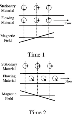
magnetically excited. Moving tissue is continuously replaced by the flow, hence velocity can be measured through the rate of decay of the signal intensity inside the same slice [224]. Velocity can also be measured through saturating a band of tissue and then following its progress in different planes [71]. The major limitation of time-of-flight methods is that the contrast of excited blood will reduce with time, eventually making it difficult to measure accurately the distances travelled. Also for cardiac studies where gating is required, only 2D images can be acquired due to the scan timing constraint. Phase flow imaging methods [77, 129] exploit principles that cause flowing material to acquire a phase shift that is related to its motion. A basic phase velocity sequence is illustrated in Figure 3.2 for a fluid flowing down a tube surrounded by stationary material.

A bipolar gradient pulse is applied, consisting first of a positive magnetic field gradient, followed a certain time later by an equal but opposite negative magnetic field gradient in the direction of the flow. During the period of the positive gradient, flowing and stationary material in a particular location will take up a frequency shift that will depend on their position in the direction of the field gradient. When the gradient is turned off, the phase of the flowing and stationary materials can be considered to be equal. In the period between the positive and negative gradients, the flowing material moves away from its stationary neighbour. During the period of the negative gradient, the stationary material will take up an equal but opposite frequency shift and return to the phase it had prior to the first gradient. However, the flowing fluid will take up a different frequency shift depending on the distance it has moved. Its final phase, therefore, also depends on this distance and hence its velocity.

Cbapter 3 Cardiac MRI Acquisition and Display

I _I

cb

Stationary

cp

_@

Material

I

I

I _I

I

Flowing

cD

Q

@

Material

j

I I I

I I

Magnetic

~

~

Field

Time 1

I _I I

Stationary

_@

_@

_@

Material

I I

Flowing

Q

Q

Q

I

----.

Material

I Flow I j I I I I

Magnetic

~

Field

~

Time 2

FIGURE 3.2: The principles of phase velocity encoding. At Time 1, a positive magnetic field gradient is applied, which results in an equal frequency and associated phase shift for neighbouring stationary and flowing spins. At Time 2, an equal but opposite magnetic field is applied. By this time, the spins in the flowing blood have moved away from their original neighbours and are now in a different strength magnetic field during gradient application. As a result, the phases of the stationary spins will be returned to zero. The flowing spins will accumulate a phase shift proportional to the distance

moved and hence the velocity.