Parallel-Interference-Cancellation-Assisted
Decision-Directed Channel Estimation
for OFDM Systems Using Multiple
Transmit Antennas
Matthias Münster and Lajos Hanzo,
Fellow, IEEE
Abstract—The number of transmit antennas that can be em-ployed in the context of least-squares (LS) channel estimation contrived for orthogonal frequency division multiplexing (OFDM) systems employing multiple transmit antennas is limited by the ratio of the number of subcarriers and the number of significant channel impulse response (CIR)-related taps. In order to allow for more complex scenarios in terms of the number of transmit antennas and users supported, CIR-related tap prediction-filter-ing-based parallel interference cancellation (PIC)-assisted deci-sion-directed channel estimation (DDCE) is investigated. New explicit expressions are derived for the estimator’s mean-square error (MSE), and a new iterative procedure is devised for the offline optimization of the CIR-related tap predictor coefficients. These new expressions are capable of accounting for the estima-tor’s novel recursive structure. In the context of our performance results, it is demonstrated, for example, that the estimator is capable of supportingL= 16transmit antennas, when assuming
K= 512subcarriers andK0= 64significant CIR taps, while LS-optimized DDCE would be limited to employingL= 8 trans-mit antennas.
Index Terms—Decision-directed channel estimation (DDCE), multiple transmit antennas, orthogonal frequency division multi-plexing (OFDM), parallel interference cancellation (PIC).
I. MOTIVATION
I
N RECENT years, the family of single- and multiuser or-thogonal frequency division multiplexing (OFDM) schemes [1] using time-domain, frequency-domain, as well as spatial-domain spreading [2] has enjoyed a renaissance. Hence, OFDM has found its way into numerous wireless systems that require accurate channel estimation. Accordingly, the topic of decision-directed channel estimation (DDCE) has been addressed in a variety of contributions, notably, for example, in the de-tailed discussions of [3]–[8], in the context of single-user single-transmit antenna OFDM environments. The basic ideaManuscript received July 3, 2002; revised October 16, 2003 and June 13, 2005; accepted June 15, 2005. The editor coordinating the review of this paper and approving it for publication is S. Roy. This work was supported by the Engineering and Physical Sciences Research Council (EPSRC), U.K., and the European Commission.
The authors are with the Department of Electronics and Computer Science (ECS), University of Southampton, Southampton SO17 1BJ, U.K. (e-mail: lh@ ecs.soton.ac.uk).
Digital Object Identifier 10.1109/TWC.2005.855793
is to equalize the channel transfer function experienced by an OFDM symbol during the current transmission period by capitalizing on that encountered during the previous OFDM-symbol period [1].1This implies assuming quasi-invariance of
the channel’s transfer function between the two consecutive OFDM symbols’ transmission intervals. An improved channel transfer-function estimate can then be obtained for detecting the most recently received OFDM symbol upon dividing the complex symbol received in each subcarrier by the sliced and remodulated information symbol hosted by a subcarrier. The updated channel estimate is then employed again as an initial channel estimate during the next OFDM symbol’s transmission period.
By contrast, channel estimation for multiuser OFDM has been considered in [9]–[15]. In the context of the multiuser OFDM scenario to be outlined in Section II, the signal re-ceived by each antenna is constituted by the superposition of the signal contributions associated with the different users or transmit antennas. Note that, in terms of the multiple-input multiple-output (MIMO) structure of the channel, the multiuser single-transmit-antenna scenario is equivalent, for example, to a single-user space-time coded (STC) scenario using multi-ple transmit antennas, provided that the channels associated with the different transmit antennas are perfectly uncorrelated. Hence, channel-estimation techniques designed for multiuser OFDM can be employed for single-user STC and vice versa. For the latter scenario, a least-squares (LS) error channel esti-mator was proposed by Liet al.[9], which aims at recovering the different transmit antennas’ channel transfer functions on the basis of the output signal of a specific reception antenna element and by also capitalizing on the remodulated received symbols associated with the different users. The performance of this estimator was found to be limited in terms of the mean-square estimation error in scenarios where the product of the number of transmit antennas and the number of channel impulse response (CIR) taps to be estimated per transmit an-tenna approaches the total number of subcarriers hosted by an OFDM symbol.
In [10], a DDCE was proposed by Jeon et al. for an STC OFDM scenario of two transmit antennas and two receive
1For sample chapters, please refer to www-mobile.ecs.soton.ac.uk.
antennas. Specifically, the channel transfer function2
associ-ated with each transmit–receive antenna pair was estimassoci-ated in the frequency domain on the basis of the output signal of the specific receive antenna upon subtracting the estimated interfering signal contributions associated with the remaining transmit antennas.
By contrast, in [11] and [13], a similar technique was pro-posed by Li with the aim of simplifying the DDCE approach of [9], which operates in the time domain. A prerequisite for the operation of this parallel interference cancellation (PIC)-assisted DDCE is the availability of a reliable estimate of the various channel transfer functions for the current OFDM symbol, which are employed in the cancellation process in order to obtain updated channel transfer-function estimates for the demodulation of the next OFDM symbol. In order to com-pensate for the channel’s variation as a function of the OFDM-symbol index, linear prediction techniques can be employed, as it was also proposed, for example, in [11]. However, due to the estimator’s recursive structure, determining the optimum predictor coefficients is not as straightforward as for a trans-versal finite-impulse response (FIR) filter-assisted predictor such as that proposed in [4]. This will be the topic of our fol-lowing discourse.
In contrast to the above backcloth, the paper proposes rank-reduced DDCE for multiuser OFDM systems supporting a high number of users. To set the scene more explicitly, channel estimation for single-user OFDM was discussed, for example, by Liet al. [9], as well as by Edfors et al.[3]. To elaborate further, the rank-reduced filtering approach, the linear predic-tive procedure along the time direction, and the PIC process have been used before in various different contexts. However, in addition to supporting a high number of multiple users, a further novel aspect of our scheme is the specific iterative method proposed for calculating the predictor’s coefficients, which can be invoked offline. This important aspect was not treated by Li in [13], since single-tap prediction filtering was considered. The predictor’s stability analysis is also new.
The outline of the papers is as follows. In Section II, we portray the signal model associated with the spatial division multiple access (SDMA) uplink transmission scenario. Note again that in terms of the MIMO structure of the channel, this SDMA system is equivalent, for example, to a single-user STC scenario employing multiple transmit antennas. Hence, the algorithms discussed here are amenable to a wide range of ap-plications involving multiple transmit antennas. In Section III, we will then focus on the PIC-assisted DDCE employing pre-diction filtering along the time axis in the CIR-related domain. Expressions are derived for the estimator’s mean-square error (MSE) and an iteration-based novel approach is devised for evaluating the optimum CIR-related tap predictor coefficients. This is followed in Section IV by an extensive performance assessment under both sample-spaced and nonsample-spaced CIR conditions. Finally, in Section V, the PIC-assisted DDCE’s complexity will be studied. Our conclusions will be offered in
[image:2.594.303.551.70.185.2]2In the context of the OFDM system, the set ofKdifferent subcarriers’ channel transfer factors is referred to as the channel transfer function, or simply as the channel.
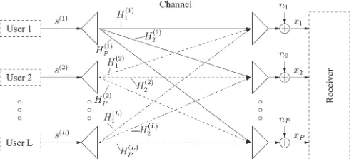
Fig. 1. Schematic of an SDMAuplinkscenario, as observed on an OFDM subcarrier basis, where each of theLusers is equipped with a single transmit antenna and the BS’s receiver is assisted by aP-element antenna front end. For comparison, in an STC scenario, theLtransmit antennas are used for providingLth-order transmit diversity for a single user. Note that, for the sake of simplicity, we have omitted the subcarrier indexk.
Section VI. In the Appendix, the conditions for the estimator’s stability are presented.
II. THESDMA SIGNALMODEL ON ASUBCARRIERBASIS
In Fig. 1, we have portrayed an SDMA uplink transmission scenario, where each of theP simultaneous users is equipped with a single transmission antenna, while the receiver capital-izes on a P-element antenna front end. The set of complex signals, xp[n, k],p= 1, . . . , P received by theP-element
an-tenna array in the kth subcarrier of the nth OFDM symbol is constituted by the superposition of the independently faded frequency-domain signals associated with theLusers sharing the same space-frequency resource. The received signal was corrupted by the Gaussian noise at the array elements. Regard-ing the statistical properties of the different signal components depicted in Fig. 1, we assume that the complex data signals(l) transmitted by thelth user has zero mean and a variance ofσ2
l.
The additive white Gaussian noise (AWGN) noise processnp
at any antenna-array element p also exhibits zero mean and a variance of σn2, which is identical for all array elements. The frequency-domain channel transfer factors Hp(l) of the
different array elements p= 1, . . . , P or users l= 1, . . . , L are independent stationary complex Gaussian distributed random variables with zero mean and unit variance, namely, σ2
H= 1.
III. ANALYTICALDESCRIPTION OFFREQUENCY-DOMAIN PIC-ASSISTEDDDCE3
The specific structure of Section III is as follows. Our portrayal of the frequency-domain PIC-assisted DDCE commences in Section III-A, where we introduce the channel-estimation algorithm. Furthermore, in Section III-B, an iterative algorithm is developed for the offline calculation of the predictor coefficients. Since normally the exact knowledge of the channel’s statistics in the form of the space–time space–frequency correlation function is unavailable, in Section III-C, we discuss potential strategies for providing estimates of the statistics required.
Fig. 2. DDCE-aided OFDM receiver.
A. Structure of the PIC-Assisted DDCE
In Section III-A1, we discuss the structure of the PIC unit. Expressions are provided both for the a posteriori channel transfer-factor estimates arrived at after the PIC, as well as for thea priorichannel transfer-factor estimates upon taking into account the effects of the CIR-related tap prediction filter. The specific structure of the predictor arrangement is detailed in Section III-A2.
1) Design of the PIC Unit: The structure of the OFDM receiver is outlined in Fig. 2 and our discussions are related to the DDCE block seen at the bottom of Fig. 2, which will be discussed in more detail in the context of Fig. 3. To elaborate a little further, following fast Fourier transform (FFT) processing, the complex frequency-domain signalx[n, k]
associated with each of theK subcarriers,k= 0, . . . , K−1, is equalized based on thea priori channel transfer-factor es-timates generated during the previous OFDM-symbol period for employment during the current period. As a result, the linear estimates sˆ[n, k] of the transmitted signals s[n, k] are obtained. These estimates are classified, yielding the complex symbols,ˇs[n, k]that are most likely to have been transmitted. The classified symbolsˇs[n, k]are then employed together with the received subcarrier signalsx[n, k]for generatinga priori
channel transfer-factor estimates for employment during the
(n+ 1)th OFDM-symbol period. The specific structure of the DDCE scheme, which is indicated by the stylized illustration at the bottom left corner, will be detailed in the paper.
Explicitly, the complex output signal xp[n, k] of the pth
receiver-antenna element in thekth subcarrier of thenth OFDM symbol is given by
xp[n, k] = L
i=1
Hp(i)[n, k]s(i)[n, k] +np[n, k] (1)
where the different variables have been defined in Section II. Upon invoking vector notation, (1) can be rewritten as
xp[n] = L
i=1
S(i)[n]Hp(i)[n] +np[n] (2)
where xp[n]∈CK×1, H(pi)[n]∈CK×1, and np[n]∈CK×1
are column vectors hosting the subcarrier-related variables xp[n, k], Hp(i)[n, k], and np[n, k], respectively, and S(i)[n]∈
CK×Kis a diagonal matrix having elements given bys(i)[n, k],
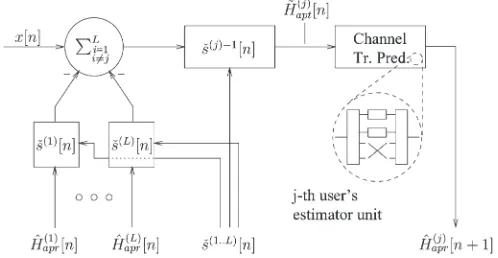
Fig. 3. Illustration of the PIC-assisted channel transfer-function estimation or prediction block, associated with thejth user and any of thePreceiver-antenna elements. The PIC process is described by (3). The structure of the channel transfer-function predictor follows the concepts of low-rank DDCE investigated in [3], [4], and [16] for the single-user scenario.
where k= 0, . . . , K−1. An a posteriori (apt) estimate
˜
H(aptj)[n]∈CK×1of the vectorH(j)[n]of “true” channel trans-fer factors between thejth user’s single transmit antenna and thepth receiver antenna can be obtained by subtracting all the
(L−1)vectors of interfering users’ estimated signal contribu-tions from the vectorxp[n]of composite received signals of the
Lusers, followed by normalization with thejth user’s diagonal matrix of detected complex symbolsSˇ(j)[n], yielding
˜
H(aptj)[n] = ˇS(j)−1[n]
x[n]−
L
i=1
i=j
ˇ
S(i)[n] ˆH(apri)[n]
(3)
where, for simplicity’s sake, we have omitted the receiver antenna’s index p.4 The PIC process based on (3) has been
further illustrated in Fig. 3. In (3), Hˆ(apri)[n]∈CK×1 denotes theith user’s vector of complexa priori(apr) channel transfer-factor estimates predicted during the(n−1)th OFDM-symbol period for thenth OFDM symbol, as a function of the vectors of a posteriori channel transfer-factor estimates H˜(apti)[n−´n]
associated with the previousNtap[t] number of OFDM symbols, which is formulated as
ˆ
H(apri)[n] =f
˜
H(apti)[n−1], . . . ,H˜(apti) n−Ntap[t]
. (4)
We will further elaborate on the specific structure of the predic-tor in the next section.
2) Design of the Predictor Unit: The channel transfer-function prediction along the time direction follows the philos-ophy of the two-dimensional (2-D) minimum MSE (MMSE) channel transfer-function-estimation approach proposed by Li et al. [4], which in turn is based on the rank-reduction-assisted one-dimensional (1-D) MMSE channel-estimation scheme proposed by Edfors and co-workers [3], [16]. A prerequisite for the optimality of these techniques was stated by Li et al. [4], arguing that the channel’s space–time
[image:3.594.307.556.72.201.2]space–frequency correlation function rH(∆t,∆f)∈C is
separable:
rH(∆t,∆f) =E{H(t1, f1)H∗(t2, f2)} (5)
=rH(∆t)·rH(∆f) (6)
where H(t, f)∈C denotes the channel’s frequency-domain transfer factor at time–frequency position(t, f)andrH(∆t)∈
C is the channel’s space–time correlation function, while rH(∆f)∈C, the space-frequency correlation function. It was
demonstrated by Li et al. [4] that this separation is valid under the assumption of uncorrelated scattering and upon fur-ther assuming that identical normalized space–time correlation functions are associated with the different paths. For further related notes, please refer to [17, Ch. 2]. Let us now briefly portray the unitary transform-based channel transfer-function predictor associated with theith user.
1) In the first step, in order to obtain the ith user’s vector of a priori channel transfer-factor estimates for the nth OFDM-symbol period during the (n−1)th OFDM-symbol period, which is denoted by Hˆ(apri)[n], the vector of a posteriori channel transfer-factor estimates H˜(apti)[n−1] is subjected to a unitary linear inverse transform U˜[f](i)H∈CK×K, yielding the
vector h˜(apti)[n−1]∈CK×1 of CIR-related a posteriori tap values:
˜
h(apti)[n−1] = ˜U[f](i)HH˜ (i)
apt[n−1]. (7)
From a statistical point of view, the optimum unitary transform to be employed is the Karhunen–Loeve trans-form (KLT) [3], [18] with respect to the Hermitian space-frequency correlation matrix of a posteriori channel transfer-factor estimates, which is given by R[aptf](i)=
E{H˜(apti)H˜(apti)H}, when assuming the wide-sense station-arity of H˜(apti)[n]. The matrix Rapt[f](i)∈CK×K can be
decomposed as R[aptf](i)=Uapt[f](i)Λapt[f](i)U[aptf](i)H, where U[aptf](i)∈CK×K is the unitary KLT matrix of eigenvec-tors, andΛ[aptf](i)∈RK×K exhibits the diagonal form of
Λ[aptf](i)= diag(λapt[f](,i0), . . . , λapt[f](,Ki)−1). The diagonal ele-ments of Λ[aptf](i) are referred to as the eigenvalues of R[aptf](i)[19]. Similarly, the desired channel’s “true” space-frequency correlation matrix R[f](i)=E{H[i]H[i]H} can be decomposed as R[f](i)=U[f](i)Λ[f](i)U[f](i)H. At this stage, we note that the error components con-taminating the vector H˜(apti)[n−1] estimating the vec-tor H(i)[n−1] of “true” channel transfer factors are uncorrelated due to the statistical independence of the AWGN and that of the modulated symbols transmitted in the different subcarriers. Hence, bothR[aptf](i)andR[f](i) share the same eigenvectors [18], which implies that we have U[aptf](i)=U[f](i). In reality, however, the explicit knowledge of the channel’s space-frequency correlation
matrixR[f](i)and that of its unitary KLT matrixU[f](i) is typically unavailable. Instead, an estimateR˜[f](i)and its associated unitary KLT matrix U˜[f](i) has to be employed, which—in contrast to the optimum KLT ma-trixU[f](i)—results in an imperfect decorrelation of the a posteriorichannel transfer-factor estimates.
2) In the second step, linearNtap[t]-tap filtering is performed in the time direction separately for thoseK0 number of CIR-related components ofh˜(apti), for which the variance is significant. This is achieved by capitalizing on the current vectorh˜(apti)[n−1]and the vectorsh˜
(i)
apt[n−n´], ´
n= 2, . . . , Ntap[t] of the previous (Ntap[t] −1) number of OFDM symbols. As a result, in the case of esti-mation filtering [4], an improved estimate hˆ(apti)[n−1]
of h(i)[n−1]is obtained, although this technique was not employed here. By contrast, in the case of the prediction filtering employed here, an a prioriestimate
ˆ
h(apri)[n]∈CK×1of h(i)[n]is obtained. In mathematical terms, this can be formulated as
ˆ
h(apri)[n] =I(Ki)0
Ntap[t] ´
n=1 ˜
cpre(i)[´n−1]˜hapt(i)[n−´n] (8)
where I(Ki)0 ∈CK×K denotes a sparse unity matrix
having unity entries only at thoseK0number of diagonal positions, for which the variance of the associated compo-nents ofh˜(apti) is significant. Furthermore, in (8), the vari-ablec˜(prei)[´n−1]∈C denotes the (´n−1)th CIR-related tap prediction-filter coefficient. Note that, for simplicity, here we employ the same coefficientc˜(prei)[´n−1]for fil-tering each of the differentK0number of taps of the spe-cificn´th CIR-related vectorh˜apt(i)[n−n´], which follows the concepts of robust channel estimation advocated by Liet al.[4].
3) In the last step, the vector of CIR-related a priori tap estimates hˆ(apri)[n] is transformed back to the OFDM frequency domain with the aid of the unitary KLT matrix
˜
U[f](i), yielding the vector ofa priorichannel transfer-factor estimates Hˆ(apri)[n] for the nth OFDM-symbol period:
ˆ
H(apri)[n] = ˜U[f](i)hˆ(apri)[n]. (9) This vector ofa priori channel transfer-factor estimates is in turn employed in the detection stage during thenth OFDM-symbol period. Upon substituting (7) into (8), and by substituting the result into (9), we obtain the following relation between the vector ofa priorichannel transfer-factor estimates derived for thenth OFDM symbol and the vectors of a posteriori channel transfer-factor esti-mates of the pastNtap[t] number of OFDM symbols:
ˆ
H(apri)[n] =T(Ki)0
Ntap[t] ´
n=1 ˜
TABLE I
SUMMARY OFPROCESSINGSTEPSASSOCIATEDWITHPIC-ASSISTEDDDCEFORMULTIPLETRANSMITANTENNASDURING THEnTHOFDM-SYMBOL
PERIOD. THELINEARFILTERINGALONG THETIMEDIRECTIONFOLLOWS THEPRINCIPLES OF AROBUSTDDCEFORSINGLE-USEROFDMAS
PROPOSED, e.g.,BYLIet al.[9]. THECALCULATION OF THEFILTERCOEFFICIENTS˜cpre(i)[´n−1],n´= 1, . . . , Ntap[t] ISCONDUCTEDWITH THEAID OF THEITERATIVEAPPROACHDEVISED INSECTIONIII-B.2, WHICH HASBEENSUMMARIZEDAGAIN,INTABLEII
whereT(Ki)0,p∈CK×Kis given by
T(Ki)
0 = ˜U [f](i)I(i)
K0 ˜
U[f](i)H. (11)
Again, the different steps of the PIC-assisted DDCE have been illustrated in Fig. 3, as well as in Table I.
After having described the process of generating the vec-tors of a posteriori and a priori channel transfer-factor es-timates in Sections III-A1 and III-A2, we will embark in Section III-B1 on an analytical evaluation of the associated
a prioriestimation MSE.
B. Derivation of an Iterative Approach for Determining the Set of Optimum Predictor Coefficients
Our discussions commence in Section III-B1 with the derivation of an expression for the averagea priori channel-estimation MSE as a function of the corresponding channel-estimation MSEs associated with the previous Ntap[t] number of OFDM symbols. This expression is then employed in Section III-B2 —under the assumption that the system is in its steady-state condition—for generating the different users’ vectors of optimum predictor coefficients, again, as a function of the predictor-coefficient-dependenta prioriestimation MSEs. Since the recursive structure of the channel transfer-function estimator does not allow for an algebraic solution to be gener-ated for the desired predictor coefficients, an iterative approach is applied, which exploits the contractive properties of the sys-tem equations. This approach was proposed earlier by Rashid-Farrokhiet al.[20] in the context of simultaneously optimizing the transmit power allocation and base-station (BS) antenna-array weights in wireless networks.
1) A Priori Channel-Estimation MSE: Let us commence our discussions in this section by developing an expression for the vector ofa priorichannel transfer-factor estimation errors associated with the jth user during the nth OFDM-symbol period as a function of the vectors of a priori channel transfer-factor estimation errors of the (L−1) remaining users during the Ntap[t] number of previous OFDM-symbol periods. Assuming error-free symbol decisions, we have
ˇ
S(j)[n−n´] =S(j)[n−n´], j= 1, . . . , L, n´= 1, . . . , N[t] tap. Substituting (2) into (3), and then substituting the result into (10), yields an expression for the vector of channel
transfer-factor estimation errors ∆ ˆH(aprj)[n]∈CK×1 in the follow-ing form:
∆ ˆH(aprj)[n] = −T(Kj)0
Ntap[t] ´
n=1 ˜
c(prej)[´n−1]S(j)−1[n−´n]
×
L
i=1
i=j
S(i)[n−n´]∆ ˆH(apri)[n−n´]
− T(Kj)
0
Ntap[t]
´
n=1 ˜
c(prej)[´n−1]S(j)−1[n−´n]n[n−´n]
+ H(j)[n]−T(Kj)0
Ntap[t] ´
n=1 ˜
c(prej)[´n−1]H(j)[n−n´] (12)
where
∆ ˆHjapr[n] =Hj[n]−Hˆjapr[n]. (13) Please observe that, for the sake of avoiding notational confu-sion, the variableiof (10) has been substituted by the variablej. The vector ofa priorichannel transfer-factor estimation errors given by (12) is constituted by three components. Specifically, the first term of (12) is due to the effects of the a priori
prediction errors of theNtap[t] number of past OFDM symbols, the second term is attributed to the contaminating effect of the AWGN, and the third term is due to the lack of “perfect predictability” of the channel transfer factors by theNtap[t]-order predictor. In other words, the last term is due to the channel transfer function’s decorrelation with time.
The average variance of the jth user’s vector of a priori
channel transfer-factor estimation errors, or equivalently, the average mean-squarea prioriestimation error, can be expressed in mathematical terms as
MSE(aprj)[n] = 1
KTrace
R∆ ˆH(j) apr[n]
(14)
whereR∆ ˆH(j) apr[n]∈C
K×K denotes the autocorrelation matrix
In the first step, let us evaluate the autocorrelation matrix R∆ ˆH(j)
apr[n]. This is achieved by substituting (12) into
R∆ ˆH(j) apr[n]
=E
∆ ˆH(aprj)[n]∆ ˆH(aprj)H[n]
(15)
= αj
σ2
j
T(Kj)0
Ntap[t] ´
n=1
˜c(prej)[´n−1]2
L
i=1
i=j
σi2R∆ ˆH(i)
apr[n−n´]|Diag
×T(Kj)H0 +αj
σ2
j
σ2n
Ntap[t] ´
n=1
˜c(prej)[´n−1]2TK(j)0T(Kj)H0 +RH(j) dec
(16)
where we introduced a new definition, namely, that of the channel transfer-function decorrelation-related matrix RH(j)
dec ∈C
K×K, which is given by
RH(j) dec
=R[f](j)−TK(j)0R[f](j)H·
˜
c(prej)HR[t](j)
−R[f](j)T(Kj)H0 ·
˜
c(prej)TR[t](j)∗
+T(Kj)0R[f](j)T(Kj)H0 ·
˜
c(prej)HR[t](j)˜c(prej)
. (17)
In the context of (16), we have exploited the fact that the three additive components of the vector∆ ˆH(aprj)[n]ofa priori chan-nel transfer-factor estimation errors in (12) are uncorrelated. The uncorrelated nature of these three terms accrues from the statistical independence of the complex AWGN process and that of the complex valued process describing the channel trans-fer function’s evolution versus frequency and time. We have also exploited the fact that the complex symbols transmitted in different subcarriers of a specific user’s signal during a specific OFDM-symbol period, as well as the symbols trans-mitted by the same user in different OFDM-symbol periods and the symbols transmitted by different users, are statistically independent, which also implies that they are uncorrelated. Still considering (16), the variableαj denotes the so-called
“mod-ulation noise-enhancement factor” [3], [21] defined as αj =
E{|s(j)[n, k]|2}E{|1/s(j)[n, k]|2}. For M-ary phase shift keying (MPSK)-based modulation schemes, such as quater-nary PSK (QPSK), we have α= 1, while for higher order quadrature amplitude modulation (QAM) schemes, we have α >1 [3], [21]. Note that here we have implicitly assumed that the same modulation scheme is employed on different subcarriers of a specific user’s transmitted signal. To elaborate further, the variables to be defined in (17) are the space–time correlation-function-related autocorrelation vector r[t](j)∈
CNtap[t]×1
of the channel transfer function, where the ´nth el-ement is given by r[t](j)|n´ =E{H(j)∗[n, k]H(j)[n−n, k´ ]}, and the space–time correlation-function-related autocorrelation matrixR[t](j)∈CNtap[t]×N
[t]
tap of the channel transfer function,
with the element(´n1,n´2)given byR[t](j)|n´1,n´2=E{H (j)[n− ´
n1, k]H(j)∗[n−n´2, k]}. Furthermore, ˜c(prej) ∈CN [t]
tap×1 is the vector of conjugate complex CIR-related tap prediction-filter
coefficients with its ´nth element given by c˜(prej)|n´ = ˜c(prej)∗[´n]. The channel’s space–frequency correlation matrixR[f](j)was defined earlier in Section III-A.2. Let us now return to our original objective, namely, that of developing an expression for the averagea priorichannel transfer-factor estimation MSE during thenth OFDM-symbol period.
In the second step, (16) is invoked in conjunction with (14) for obtaining an expression for thejth user’s averagea priori
channel transfer-factor estimation MSE as a function of the remaining users’a prioriestimation MSEs associated with the Ntap[t] number of previous OFDM-symbol periods:
MSE(aprj)[n] =
K0
K αj
σ2
j Ntap[t]
´
n=1
˜c(prej)[´n−1] 2L
i=1
i=j
σi2MSE
(i) apr[n−´n]
+K0
K αj
σ2
j
˜c(prej)2
2σ 2 n+MSE
(j) dec (18)
where we have
MSE(decj) = 1
KTrace
RH(j) dec
(19)
= σH2 − 1
KTrace
Υ[f](j)I(Kj0)
×2Re
˜
c(prej)Hr[t](j)
− ˜c(prej)HR[t](j)c˜(prej)
. (20)
In the context of deriving (18), we have capitalized on the relations Trace(A+B) =Trace(A) +Trace(B), as well as on Trace(UAUH) =Trace(A), which are valid for a unitary matrix U [18], [22]. Furthermore, in the context of deriving the first additive term in (18), we exploited the fact that (1/K)Trace(TK(j)0R∆ ˆH(i)
apr[n−´n]|DiagT (j)H
K0 ) = (K0/K)MSE
(i)
apr[n−´n], which is only valid for a unitary transform matrixU˜[f](j)having elements of unity magnitude. This is the case, for example, when employing the discrete FT (DFT) matrixWas the unitary transform matrix. The second additive term in (18) is based on exploiting the relationship of (1/K)Trace(TK(j0)T(Kj)H0 ) =K0/K. We also note in this context thatT(Kj)H0 =TK(j0), and thatTK(j)0T(Kj0)H=T(Kj)0.
Furthermore, in (20), the matrix Υ[f](j)∈CK×K denotes the decomposition of thejth user’s channel’s space–frequency correlation matrix R[f](j) with respect to the unitary trans-form matrix U˜[f](j), which is expressed as Υ[f](j)=
˜
U[f](j)HR[f](j)U˜[f](j). Note that in contrast toΛ[f](j) associ-ated with the decomposition ofR[f](j)with respect toU[f](j), the matrix Υ[f](j) is not necessarily of diagonal shape, con-strained to having real-valued elements only.
2) Iterative Calculation of the CIR-Related Tap Predictor Coefficients: In the steady-state condition, we can assume that the specific user’sa priorianda posterioriestimation MSEs are identical for different OFDM symbols, which is expressed as
where i= 1, . . . , L and n´= 0, . . . , Ntap[t] . Hence, (18) simplifies to
MSE(aprj) =K0
K αj
σ2
j
˜c(prej)2
2 × L i=1
i=j
σi2MSE(apri) +σ2n
+MSE(decj). (22)
Upon invoking (22), thejth user’s vector of CIR-related tap predictor coefficients ˜c(prej) can be evaluated conditioned on the remaining (L−1) number of users’ a priori estimation MSEs, namely on MSE(apri),i= 1, . . . , L, i=j, which ensues by calculating the gradient of MSE(aprj) with respect to thejth user’s coefficients, yielding
∇(j)MSE(j) apr= K0 K αj σ2 j ˜
c(prej)
L i=1
i=j
σi2MSE(apri) +σ2n
−1 KTrace
Υ[f](j)I(Kj)0
×r[t](j)−R[t](j)˜c(prej)
(23)
where R[t](j) and r[t](j) were defined in the context of (17). The gradient vector, with respect to thejth user’s coefficients, is defined here as ∇(j)=∂/(∂˜c(prej)∗). In the context of (23), we have exploited the fact that∇(j)˜c(prej)H =I, as well as the fact that∇(j)˜c(j)T
pre =0and∇(j)(˜c(prej) 2 2) = ˜c
(j) pre[19].
In the optimum point of operation, we have∇(j)MSE(j) apr=
0 and hence, (23) can be solved for the jth user’s vector of predictor coefficients, resulting in the Wiener-filter-related solution of5
˜
c(prej)|opt=
R[t](j)+ K0
Trace
Υ[f](j)I(j)
K0 αj σ2 j × L i=1
i=j
σ2iMSE(apri) +σn2
I −1
·r[t](j). (24)
Based on (22) and (24), a fixed-point iteration algorithm [19] can be devised for obtaining the different users’ vectors of
5Note that in the context of identical transmit powers, modulation modes, and channel statistics, (24) is significantly simplified, namely, we obtain the same vector of predictor coefficients given by˜cpre|SIMPLEopt = [R[t]+ (K0/Trace(Υ[f]I
K0)) α((L−1)MSEapr|
SIMPLE+ (σ2
n/σs2))I]−1·r[t], as well as the same average estimation MSE for the different users. Fur-thermore, note that upon removing the (L−1) number of contributions, which are related to the PIC process, we then obtain the expressions for the estimation MSE and the vector of coefficients associated with a trans-versal predictor, which can be expressed as ˜cpre,FIR|SIMPLEopt = [R[t] + (K0/Trace(Υ[f]I
K0))α(σ
2
n/σ2s)I]−1·r[t].
predictor coefficients under the constraint of minimizing the sum of the different users’ a priori estimation MSEs. This approach was proposed earlier by Rashid-Farrokhiet al. [20] in the context of simultaneously optimizing both the transmit power allocation and the base-station antenna-array weights in wireless networks, leading to formulas similar to (22) and (24). In our forthcoming discourse, we will briefly present the steps of the algorithm with respect to our specific optimization problem, but for a formal proof of the algorithm’s convergence and that of the uniqueness of the solution, we refer to [20]. Note that, in the context of our description of the algorithm, the iteration index—and not the OFDM-symbol index—is given in the square brackets.
1) Initialize the different users’ a prioriestimation MSEs, for example, by setting MSE(aprj)[0] = 0forj= 1, . . . , L. 2) For thenth iteration: Conditioned on thea priori estima-tion MSE values obtained during the(n−1)th iteration, namely, on MSE(aprj)[n−1],j = 1, . . . , L, calculate the different users’ vectors of optimum predictor coefficients for thenth iteration, namely,˜c(prej)[n]|opt,j= 1, . . . , L, with the aid of (24).
3) Conditioned on the nth iteration’s predictor-coefficient vectors˜c(prej)[n]|opt,j= 1, . . . , L, obtained in step 2) and also conditioned on the (n−1)th iteration’s a priori
estimation MSE values, namely on MSE(aprj)[n−1],j= 1, . . . , L, calculate thenth iteration’sa prioriestimation MSE values of MSE(aprj)[n], j= 1, . . . , L, with the aid of (22).6
4) Start a new iteration by returning to step 2).
The essential equations of this optimization procedure have been summarized again in Table II. Note that, instead of invoking (22) separately for each user, the different users’
a priori estimation MSEs can also be calculated in parallel with the aid of (33), as a result of which, an even faster convergence is achieved. The price to be paid is a higher computational complexity, since an explicit matrix inversion is required in (33).
In the next section, we will address the problem of a potential lack of knowledge about the channel’s exact statistics, namely, that of the space–time space–frequency correlation function.
C. Channel Statistics
As it was observed in (22) and (24), a prerequisite for deter-mining the different users’ vectors of optimum CIR-related tap predictor coefficients is the knowledge of the users’ space–time
6Recall that the representation of thejth user’s estimation MSE was valid only when assuming that the unitary transform matrixU˜[f]has elements of unity magnitude, which is the case, for example, for the DFT matrix W. However, in the more general scenario of employing an arbitrary unitary transform matrix, which could be, for example, one of the robust transforms proposed in [23], this condition is not fulfilled. In this case, the matrix
R
∆ ˆH(aprj)[n]has to be explicitly iterated with the aid of (16), upon assuming R
TABLE II
SUMMARY OFPROCESSINGSTEPSASSOCIATEDWITH THEOPTIMIZATION OF THEPIC-ASSISTEDDDCE’SPREDICTORCOEFFICIENTS
channel transfer-factor correlation functions r[Ht](j)[∆n], j= 1, . . . , L, defined by
rH[t](j)[∆n] =E
H(j)[n, k]·H(j)∗[n−∆n, k]
. (25)
These are required for evaluating the autocorrelation matrices R[t](j) and cross-correlation vectorsr[t](j), for j= 1, . . . , L. Assuming Jakes’ fading model [24] for example, the channel correlation along the time direction is given by [4]
rH,J[t](j)[∆n] =J0
∆n·ωD(j)
(26)
≈1−1 4
∆n·ωD(j)
2
, ∆n·ω(Dj)1 (27)
where J0() denotes the zero-order Bessel function of the first kind and ωD(j)= 2πTffD(j), and Tf being the
OFDM-symbol duration including the guard period time, while fD(j) denotes the channel’s Doppler frequency. Since usually the exact Doppler frequencyfD(j)is not known, it was demonstrated in [4], in the context of a transversal-type estimator, that the MSE performance degradation incurred due to a mismatch of the channel statistics is only marginal, if a uniform ideally support-limited Doppler power spectrum associated with
˜
fD(j)≥fD(j) is assumed for the calculation of the correlation coefficients of (25). The associated space–time correlation function is given as the inverse FT of the uniform Doppler power spectrum, which leads to
˜
r[H,t](unifj) [∆n] = sin
∆n·ω˜D(j)
∆n·ω˜(Dj) . (28)
Furthermore, the calculation of the vectors of CIR-related tap predictor coefficients according to (24) also requires the evalu-ation of the expression Trace(Υ[f](j)I(j)
K0). More explicitly, we recall from Section III-A2 that Υ[f](j) is the decomposition of thejth user’s channel’s space–frequency correlation matrix R[f](j) with respect to the unitary transform matrix U˜[f](j), which is formulated as Υ[f](j)= ˜U[f](j)HR[f](j)U˜[f](j), and
I(Kj)
0 is a sparse identity matrix having unity entries only at
those K0 number of positions, which are associated with a significant value ofΥ[f](j). Hence, we note that the evaluation of Trace(Υ[f](j)I(j)
K0)requires the knowledge ofR
[f](j), which is not directly available in practice.
A viable approach is that of obtaining an “average” value of Trace(Υ[f](j)I(j)
K0)by employing the space–frequency correlation matrix R˜[f](j) based on the space–frequency cor-relation function associated with a uniform ideally support-limited multipath intensity profile.7The sparse identity matrix
I(Kj)0 could be designed for retaining the firstK0 CIR-related coefficients of Υ[f](j)—rather than the K
0 largest one—or alternatively, for retaining the firstKI
0 and the lastK0II CIR-related coefficients of Υ[f](j), where K
0=K0I +K0II. This was suggested by van de Beeket al.[25] in the context of DFT-based channel transfer-function estimation employed designed for single-user OFDM systems.
IV. PERFORMANCE
With the exception of the results to be presented in Section IV-B, our investigations were conducted for an SDMA uplink scenario supporting four simultaneous equal-power OFDM users, each equipped with one transmit antenna. At the BS, four reception antennas were assumed. Furthermore, for the sake of simplicity, the different users were assumed to employ the same modulation scheme, and the channels between the different transmit antennas and each receiver antenna were assumed to have the same Doppler power spectrum.8 Unless
otherwise stated, the specific channel statistics invoked were that of the channel’s space–time correlation function provided by the Jakes model, as given by (26), having an OFDM-symbol-normalized Doppler frequency9ofFD= 0.007, which corresponds to a vehicular speed of 50 km/h, or equivalently,
7The continuous unit-energy uniform power delay profile is given by
rh,unif(τ) = (1/Tm)rect(τ−τshift/Tm), while its FT, namely the space-frequency correlation function, is given byrH,unif(∆f) = sin(πTm∆f)· e−j2πτshift∆f.
8Recall that in this scenario, (24) and (33), associated with the iterative
optimization of the predictor coefficients, as proposed in Section III-B2, are significantly simplified.
9The OFDM-symbol-normalized Doppler frequency is defined as FD=
fDTf, wherefDis the Doppler frequency andTf denotes the OFDM symbol
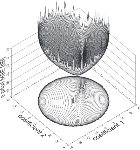
Fig. 4. Evolution of thea priorichannel-estimation MSE according to (33), as a function of the real-valued coefficients of the two-tap CIR-related tap predictor employed in this particular example. The number of subcarriers was K= 512, while the number of significant CIR-related taps wasK0= 16, in the context of a sample-spaced CIR. Furthermore, the number of users was L= 4and the OFDM-symbol-normalized Doppler frequency wasFD= 0.1. The space-time channel correlation function of (28), associated with a uniform ideally support-limited Doppler power spectrum, was invoked. The SNR at the reception antenna was equal to 20 dB.
31.25 mi/h in the context of the indoor wireless asynchronous transfer mode (WATM) system’s parameters [1], [26] invoked here.10 Furthermore, we considered “frame-invariant” fading, where the fading envelope of each CIR-related tap has been kept constant during each OFDM symbol’s transmission period. This avoided the obfuscating effects of intersubcarrier inter-ference and hence, enabled us to study the various channel transfer-function-estimation effects in isolation. Furthermore, apart from our investigations in Section IV-G, error-free symbol decisions were assumed in the generation of the remodulated reference used for DDCE.
A. Evolution of the A Priori Channel Estimation MSE in a 2-Tap CIR-Related Tap Prediction Scenario
In Fig. 4, we have exemplified the evolution of the aver-agea priorichannel transfer-factor estimation MSE according to (33), as a function of the CIR-related tap predictor coeffi-cients’ associated values, where we employed a two-tap predic-tor, since for a higher number of predictor taps, a visualization
10Note that associated with the indoor WATM channel is a sample-spaced CIR having a multipath spread ofTm= 12Ts. In the context of our simula-tions, which employed the indoor WATM channel’s CIR, the matrixI(Kj)
0was designed such as to retain the firstK0number of CIR-related taps. Hence, in case thatK0>12, we have Trace(Υ[f](j)I(j)
K0) =Kσ
2
[image:9.594.45.290.69.332.2]H.
Fig. 5. A priori channel-estimation MSE versus SNR performance exhib-ited by the PIC-assisted DDCE of Fig. 3, using the optimum recursive predictor coefficients evaluated with the aid of the iterative approach of Section III-B2. As a benchmarker, we have plotted the a priori channel-estimation MSE performance achieved with the aid of the suboptimum transversal predictor coefficients. Each of the SDMA scenario’s independently faded channels is characterized by the indoor WATM channel parameters of [1] and [26].
is less convenient. Also, note that the predictor coefficients are real valued due to the employment of the real-valued space–time channel correlation function of (26). In our partic-ular example, the a priorichannel-estimation MSE evaluated from (33) is minimized for a coefficient vector of ˜cpre|opt≈ (1.771,−0.898)T. By contrast, for coefficient pairs outside the circle having a radius of K/K0α(L−1)≈3.27, centered around the origin of the R2 space, the channel estimator is unstable, which is evidenced by an excessive MSE.
B. Influence of the Number of Simultaneous Users on the A Priori Channel-Estimation MSE
In this section, we will demonstrate that the PIC-assisted approach advocated here is capable of supporting scenarios of a higher complexity in terms of theLnumber of simultaneous users, than a maximum of Lmax=K/K0, as supported by the LS-assisted DDCE of [9]. Hence, in Fig. 5, we have plotted the average a priori channel transfer-factor estimation MSE of the PIC-assisted DDCE as a function of the L number of simultaneous users, assuming an eight-tap CIR-related tap prediction filter and a fixed number of K0= 64 significant CIR-related taps. This corresponds to 12.5% of the duration of a 512-subcarrier OFDM symbol’s time-domain representation, which may be viewed as the relative upper bound of the CIR length in a well-designed OFDM system. Here, we capitalized again on the idealistic assumption of encountering error-free symbol decisions. We observe in Fig. 5 that the
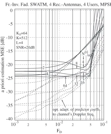
Fig. 6. A priorichannel-estimation MSE versus OFDM-symbol-normalized Doppler-frequency performance exhibited by the PIC-assisted DDCE of Fig. 3, using optimum recursive predictor coefficients. The predictor coefficients were optimized forF˜D= 0.05, using the iterative approach of Section III-B2. As in previous graphs, a Jakes’s spectrum-related space-time correlation function obeying (26) was associated with the channel. Each of the SDMA scenario’s independently faded channels is characterized by the indoor WATM channel parameters of [1] and [26].
because more multiuser interference-related noise is inflicted by thea posteriorichannel estimates during the PIC process, which is then injected into the a priori channel estimates’ prediction process. However, these effects can be mitigated by increasing the predictor’s range. Again, we observe that, in the context of the suboptimum transversal predictor coefficients of footnote 5, the PIC-assisted DDCE tends to become unstable at higher signal-to-noise ratios (SNRs).
C. Influence of a Mismatch of the OFDM-Symbol-Normalized Doppler Frequency
In Fig. 6, we have portrayed the average a priori chan-nel transfer-factor estimation MSE versus OFDM-symbol-normalized Doppler-frequency performance of the recursive es-timator of Fig. 3, in the context of employing a uniform ideally support-limited Doppler power spectrum having a space–time correlation function obeying (28) in the calculation of the CIR-related tap predictor coefficients. Furthermore, a Doppler power spectrum obeying Jakes’s model [24] and having a space–time correlation function given by (26) was associated with the channel. In our particular example, the predictor coefficients were calculated upon invoking once again the iterative approach of Section III-B2 for an OFDM-symbol-normalized Doppler frequency ofF˜D= 0.05. Furthermore, as a reference, we have also plotted thea priorichannel-estimation MSE performance in the context of predictor coefficients, which were optimized for the channel’s specific Doppler frequency. As reported in [4] and also observed in Fig. 6, upon increasing the number of predictor taps, thea priorichannel-estimation MSE is
ren-dered quasi-invariant for OFDM-symbol-normalized Doppler frequencies, which are lower than that assumed in the cal-culation of the CIR-related tap predictor coefficients, namely
˜
FD= 0.05. By contrast, for higher Doppler frequencies, a rapid degradation of the MSE is observed in Fig. 6. This “robustness” is achieved at the cost of a potentially significant loss in performance compared to the case of optimally adapted predictor coefficients. To give an example, it is seen in Fig. 6 that for an SNR of 20 dB and for 64 predictor coefficients, the
a priorichannel-estimation MSE performance loss is as high as 10 dB at an OFDM-symbol-normalized Doppler frequency ofFD= 0.007, when the predictor coefficients were designed forF˜D= 0.05.
D. Effects of Correlated Domain Leakage Upon Assuming a Uniform Nonsample-Spaced CIR11
Our analytical evaluations in the previous sections were conducted so far under the assumption of a sample-spaced CIR. Using a sample-spaced CIR facilitates the recovery of almost all the energy of the channel’s output, upon invoking a finite number ofK0< K significant taps. By contrast, in the context of the more realistic scenario of a nonsample-spaced CIR, the energy conveyed by the channel is distributed over a higher number of CIR-related taps, i.e., it potentially “leaks” to all CIR-related taps.
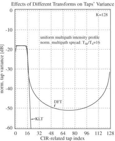
In order to demonstrate the effects of leakage, in Fig. 7, we have plotted the normalized variance of the diagonal elements of the decomposition of R[uniff] based on the space–frequency correlation function rH,unif(∆f)associated with the uniform multipath intensity profile,12 when employing the DFT matrix
W as the unitary transform matrix U˜[f], which is expressed mathematically as Υ[uniff] = ˜U[f]HR[f]
unifU˜[f]. The “u”-shaped evolution of the tap variances seen in Fig. 7 for tap indices in excess of Tm/Ts= 16 is, again, a result of the leakage incurred. By contrast, in the context of decomposing the matrix R[uniff] with the aid of the optimum KLT matrix, namelyΛ[uniff] =
U[uniff]HR[uniff] U[uniff] , the channel’s energy is concentrated on a number of CIR-related taps, which is only slightly higher [3] than the multipath spreadTmnormalized to the sampling period durationTs, as observed in Fig. 7.
E. A Priori Channel-Estimation MSE for a Nonsample-Spaced Uniform CIR13
The correspondinga priorichannel-estimation MSE curves, which were evaluated with the aid of the iterative approach of Section III-B2, are plotted in Fig. 8, as a function of the K0 number of significant CIR-related taps. The factor (K0/Trace(Υ[f](j)I(Kj)0))of (24) was evaluated upon selecting 11The normalized multipath spread was set equal to one eighth of the
K= 512subcarriers assumed here, namely, toTm/Ts= 64.
12The continuous unit-energy uniform power delay profile is given by
rh,unif(τ) = (1/Tm)rect(τ−τshift/Tm), while its Fourier transform, namely the space-frequency correlation function, is given byrH,unif(∆f) = sin(πTm∆f)·e−j2πτshift∆f.
13The normalized multipath spread was set equal to one eighth of the
Fig. 7. Illustration of the normalized variance associated with the diagonal elements of the decompositionΥ[f]= ˜U[f]HR[f]U˜[f]ofR[f]with respect toU˜[f]=Wand of the decompositionΛ[f]=U[f]HR[f]U[f]with respect to the optimum KLT matrixU[f], in the context of a uniform multipath intensity profile, having a normalized multipath spread ofTm/Ts= 16. The normalization of the diagonal elements ofΥ[f]was carried out with respect to theK= 128number of subcarriers.
theK0largest tap variances from the decompositionΥ[uniff](j)= ˜
U[f](j)HR[f](j)
unif U˜[f](j) of the specific space–frequency corre-lation matrices of the channel with respect toU˜[f](j)=W.14
The curves are also parameterized with the Ntap[t] number of predictor taps. A rapid improvement of the estimator’s MSE is observed upon increasing theK0 number of significant CIR-related taps up to a certain optimum K0 value, which is a consequence of retaining more of the channel’s energy. At the same time, more of the undesired noise is retained, since a gradually decreasing fraction of the CIR-related taps are discarded. Upon increasing theK0number of significant taps beyond the optimum point seen in Fig. 8, the opposite behavior is observed, namely, that the MSE is degraded again. This is because for these taps, the benefit of extracting more of the channel’s energy is lower than the penalty incurred due to retaining more of the undesired noise. Note that this behavior is a result of employing the same set of predictor coefficients for the filtering of each of the different CIR-related taps. By contrast, in the context of a predictor arrangement employing individually optimized sets of coefficients for the prediction of each of the different CIR-related taps, a “leveling out” of thea prioriestimation MSE performance would be observed, instead of the explicit degradation seen in Fig. 8. This is because for the low-energy CIR-related taps suffering from a low
channel-14Note that while for the sample-spaced CIR we have Trace(Υ[f](j)I(j)
K0) =
Kσ2
HforK0< K upon appropriately selectingI
(j)
K0, in the context of the nonsample-spaced CIR, we potentially have Trace(Υ[f](j)I(j)
K0)< Kσ
2
Hfor
[image:11.594.76.261.67.294.2]K0< K, which results from the leakage.
Fig. 8. A priori channel-estimation MSE performance of the PIC-assisted DDCE of Fig. 3, using optimum recursive predictor coefficients, versus the K0 number of significant CIR-related taps retained in the context of a uni-form multipath intensity profile, having a normalized multipath spread of Tm/Ts= 64. The DFT matrixU˜[f]=Wwas employed as a transform basis.
related signal-component-to-noise ratio, the noise would be more mitigated.
F. A Priori Channel Transfer-Factor Estimation MSE for a Nonsample-Spaced CIR on a Subcarrier Basis
The specific distribution of the a priori channel transfer-factor estimation MSE across the different subcarriers can also be obtained using the approach outlined in Section III-B2 for jointly optimizing the averagea priorichannel-estimation MSE and the predictor coefficients.
However, this involves invoking (16) instead of (22) in the algorithm outlined above. Again, in the context of a stable operation, as defined in the Appendix, we assume that the estimator’s statistics recorded in the form of the a priori
channel transfer-factor estimation errors’ correlation matrix R∆ ˆH(j)
apr[n] =R∆ ˆH (j)
apr[n−´n]is invariant for´n= 1, . . . , N [t] tap, yielding
R∆ ˆH(j) apr[n] =
αj
σ2
j
˜c(prej)
2
2T (j)
K0
×
L
i=1
i=j
σ2iDiag
R∆ ˆH(i) apr[n]
+σ2n
T(Kj)H0 +RH(j) dec
. (29)
Recall that the desired subcarrier-based a priori channel transfer-factor estimation MSE variances are found on the main diagonal of the matrix R
∆ ˆH(aprj)[n] of (29). The iter-ation commences with an initial assignment for the matri-ces R∆ ˆH(j)
Fig. 9. A priorichannel-estimation MSE performance versus the subcarrier index exhibited by the PIC-assisted DDCE of Fig. 3, using optimum recursive predictor coefficients. The DFT matrixU˜[f]=Wwas employed as a trans-form basis.
Thejth user’sa priorichannel transfer-factor estimation-error correlation matrix is then updated with the aid of (29), on the basis of the remaining users’ error correlation matrices’ diagonals, denoted by Diag{R∆ ˆH(i)
apr[n]}, employing the re-maining users’ associated current vectors of predictor coef-ficients. After updating all users’ error correlation matrices, the vectors of predictor coefficients are updated with the aid of (24). This involves evaluating first the average a priori
channel transfer-factor estimation MSEs with the aid of (14), on the basis of the updated error correlation matrices. The iteration continues by updating the error correlation matri-ces, again, upon invoking the updated vectors of predictor coefficients.
Our analytical performance evaluations have been carried out for the uniform multipath intensity profile, again, in con-junction with a normalized multipath spread of Tm/Ts= 64 and for K= 512 subcarriers. The number of predictor taps wasNtap[t] = 4. Our simulation results are portrayed in Fig. 9 for an SNR of 20 dB recorded at the reception antennas. The curves are further parameterized with theK0 number of sig-nificant CIR-related taps. As also evidenced by the simulation results of Fig. 8, the value of K0 should be in excess of
Tm/Ts= 64 in order to be able to extract all the significant taps and hence, to prevent an excessive degradation of the MSE. The most important observation drawn from Fig. 9 is that, as a result of the effects of leakage imposed by the uniform multipath intensity profile, the estimation MSE is sub-stantially degraded for the outer subcarriers of the frequency-domain OFDM symbol. Estimation MSEs as high as−5 dB are observed. Based on the relatively high MSE associated with the outer subcarriers, we also expect, for these subcar-riers, a significantly deteriorated bit error rate (BER) perfor-mance, compared to the subcarriers at the center of the OFDM symbol.
Fig. 10. BER versus SNR performance of an uncoded system employing the PIC-assisted DDCE of Fig. 3, using optimum recursive predictor coefficients in conjunction with both MMSE and M-SIC(M= 2)-based detection at the receiver. The fraction of training overhead imposed was either 6.25% or 100%, which corresponds to transmitting one dedicated training OFDM symbol per every block of 16 OFDM symbols, while the latter denotes the idealistic case of an error-free reference. Each of the SDMA scenario’s independently faded channels is characterized by the indoor WATM channel parameters of [1] and [26].
G. System BER in the Context of Imperfect Error-Contaminated Symbol Decisions Assuming a Sample-Spaced CIR
So far, in this section, we have capitalized on the idealistic assumption of error-free symbol decisions. By contrast, in a realistic scenario, the channel-estimation process is impaired by erroneous symbol decisions. These effects will be further highlighted during our forthcoming discussions.
[image:12.594.333.516.66.291.2]