Field Phenotyping for the Future 1
2
Jonathan A Atkinson1*, Robert J Jackson2*, Alison R Bentley2, Eric Ober2 and Darren M Wells1 3
4
1School of Biosciences 5
University of Nottingham
6
Sutton Bonington
7
UK
8
9
2The John Bingham Laboratory, 10
NIAB
11
Huntingdon Road
12
Cambridge
13
UK
14
15
*these authors contributed equally
16
Corresponding author: Darren M. Wells ([email protected])
17
18
Abstract 20
Global agricultural production has to double by 2050 to meet the demands of an increasing
21
population and the challenges of a changing climate. Plant phenomics (the characterization
22
of the full set of phenotypes of a given species) has been proposed as a solution to relieve the
23
“phenotyping bottleneck” between functional genomics and plant breeding studies. In this
24
review, we survey current approaches and describe recent technological and methodological
25
advances for phenotyping under field conditions and discuss the prospects for these emerging
26
technologies in addressing the challenges of future plant research.
27
28
29
Keywords 30
Field phenotyping, phenomics, sensors, phenotyping platforms
31
1.1Introduction 33
A doubling of global agricultural production is required by 2050 to meet the demands of an
34
increasing population and the challenges of a changing climate (Alexandratos and Bruinsma,
35
2012). This production increase will need to be met by more intensive use of the same land
36
area through the priority process of sustainable intensification. An aspect of this requires a
37
hastening of the plant breeding effort to deliver increased potential yields. However,
38
potential yields are not always achieved on farm, and growing attention is paid to the
39
stagnation of crop yields on farm (Ray et al., 2012). Elements of understanding and driving
40
both plant breeding gain and on-farm productivity rely on the accurate capture of the
41
phenotypic response and performance. At its broadest this encompasses harvestable yield
42
and crop quality, as well as agronomic, biotic and abiotic stress tolerance characters. At a finer
43
scale it involves the precision analysis of phenotypes for the dissection of underlying plant
44
processes.
45
Much progress has been made over the past decade in decoding and describing the genetics
46
of key plant species. This encompasses the development of molecular markers for use in
47
marker-assisted selection to accelerate breeding gain through to the generation of whole
48
genome assemblies giving unprecedented insight into the genomes of crop species. These
49
advances have also been enabled with rapid advances in bioinformatics and the development
50
of software tools and other computational resources to allow the extraction and application
51
of genetic and genomic data.
52
In comparison, developments in the detailed understanding of plant phenotypes has been
53
slow. The field of plant phenomics (the characterization of the full set of phenotypes of a
54
given species) has been proposed as a solution to relieve the so-called “phenotyping
55
bottleneck” between functional genomics and plant breeding studies (Furbank and Tester,
56
2011). This encompasses both the capture of plant phenotypes using a range of
57
methodologies and the accurate and timely extraction, analysis and application of the
58
resulting data. Although relatively well developed in controlled conditions (Bai et al., 2016),
59
progress in understanding and interrogating complex phenotypes at the field level remains
60
slow. In this review, we survey recent advances in phenotyping under field conditions and
61
discuss the prospects for these emerging technologies in addressing the challenges of plant
62
research for the future.
64
1.2Traditional field phenotyping approaches 65
Through the empirical selection of favourable individuals for harvest, consumption and
66
replanting, early farmers employed the most traditional of phenotyping approaches: physical
67
appearance of a plant in its environment. Early selection led to the subsequent domestication
68
of many crop species. Studies in barley have shown the spread of favourable mutations
69
modifying response to the seasonal daylength queue for the initiation of reproductive
70
development supported the Neolithic spread of the crop for cultivation (Jones et al., 2008).
71
Farmers and breeders have continued to use phenotypic selection in an environment, or
72
series of environments, through time. Beyond domesticating wild species this has allowed in
73
particular, for the optimisation of key adaptive traits, including flowering time to ensure
74
maximum yields in a given region. Driven by physical appearance as the result of both genetic
75
and environmental effects, this process has indirectly selected a complex of underlying
76
genetic controllers. Modern plant science and breeding still rely on traditional phenotyping
77
tools. This ranges from simple measurements of growth (e.g., height), time series
78
measurements of the appearance of development stages (e.g., vegetative and reproductive
79
development), comparative numerical scores or indices (e.g., for assessment of pest or
80
pathogen infection) through to assessment of agronomic performance (e.g., yield, biomass)
81
and predictive tests (e.g., for end-use quality traits). When employed at scale and with
82
sufficient replication, many of these traits can be assessed reliably, supporting subsequent
83
selection or analysis. This is particularly true for simple traits that have a high heritability
84
(Hallauer et al., 2010).
85
Estimation of the genotypic value of a large number of selection candidates (in plant breeding)
86
or cultivars to be recommended to farmers (in variety testing and agronomy) is central to
87
breeding and/or crop production (Piepho et al., 2008). Heritability is a driver of this
88
estimation: defining the degree to which phenotypic variance is a result of genetic variation.
89
Irrespective of the means of generating phenotypic data, its heritability will impact the degree
90
to which it can be used as a selection or trait discovery tool.
91
Confounding this is genotype-by-environment interactions, which have been reviewed
92
extensively elsewhere (e.g. Yan & Hunt, 2010). The magnitude of climate change effects on
93
crops are likely to be, in part, cultivar dependent, necessitating practical solutions to tailor
selective breeding to changing regional patterns (Trnka et al 2014). In order to reliably devise
95
production strategies under future climatic uncertainty, trade-offs to physiologically-based
96
plant processes and productivity across environments need to be accurately characterised
97
which expands the need for development and application of accurate and high-throughput
98
field phenotyping capabilities.
99
100
1.3High-throughput field phenotyping platforms 101
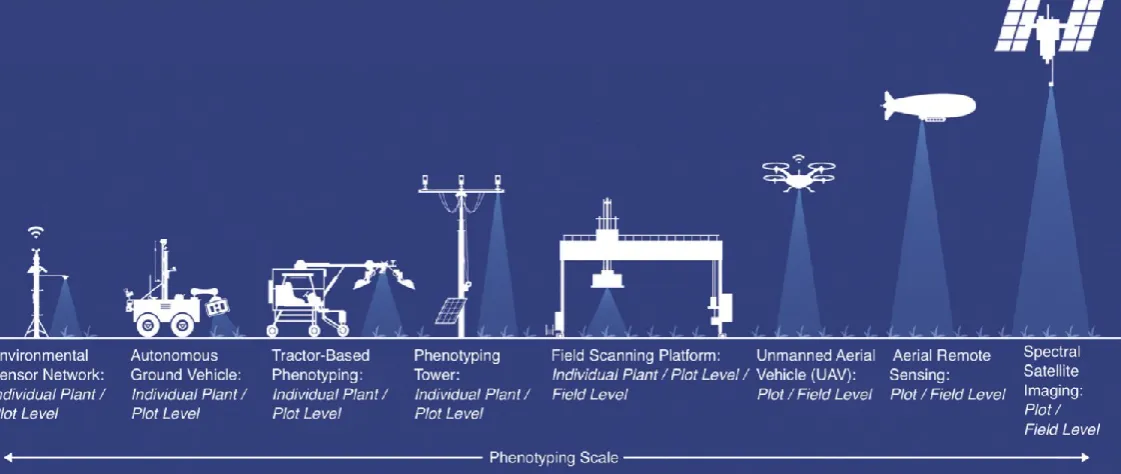
High-throughput plant phenotyping can be delivered in the field via a variety of platforms,
102
across a range of scales (see Figure 1 for examples) and using a diverse array of sensor
103
modalities (Araus and Cairns, 2014). Platforms can be broadly classified as those operating at
104
ground-level (both above and below the soil surface) and those operating aerially (air- or
105
space-borne). The appeal of these platforms is the increased throughput and impartiality with
106
which they collect data when compared to traditional field approaches.
107
1.3.1Above-ground phenotyping platforms 108
In comparison to phenotyping under controlled conditions, where the movement of either
109
sensors or plants can be automated to increase throughput, ground-based plant field
110
phenotyping requires either a network of fixed sensors or a system to move sensors over the
111
crop. The simplest systems operate at the lowest spatial resolution (single plants or
112
experimental plots) and consist of fixed platforms typically monitoring the local environment
113
and imaging crop development using visible light cameras (Naito et al., 2017; Zhou et al.,
114
2017). These systems have the advantage of being relatively inexpensive, allowing
115
deployment of multi-unit networks to increase throughput to the whole-field level (Zhou et
116
al., 2017).
117
Multiple plots can be assessed using mobile platforms, the simplest of which are wheeled
118
buggies or “phenocarts”- hand-propelled platforms capable of deploying heavier sensor
119
payloads than can be carried by an individual user (White and Conley, 2013). Motorised
120
versions of the cart design have been developed that, although still requiring an operator,
121
allow high-throughput positioning of sensor arrays across an experimental field (Deery et al.,
122
2014; Jimenez-Berni et al., 2018). Fully-autonomous ground vehicles (ranging in size from
123
small robots capable of navigating between row crops to tractor-sized vehicles) offer the
promise of unattended field monitoring and have been the focus of much recent research
125
(Shafiekhani et al., 2017; Underwood et al., 2017; Burud et al., 2017; Grimstad and From,
126
2017). Trailer or tractor-mounted systems have the benefit of utilising precision agriculture
127
platforms already present at most field sites and have been extensively used for row crops
128
(Comar et al., 2012; Busemeyer et al., 2013; Fernandez et al., 2017; Tanger et al., 2017).
129
Drawbacks of tractor-based systems (and heavier autonomous ground vehicles) are that they
130
cannot be deployed in adverse weather or soil conditions and that repeated traversing of the
131
field may lead to unwanted soil compaction, impacting plant development (Virlet et al., 2017).
132
Compaction can be avoided by use of larger versions of fixed platforms (often termed
133
“phenotyping towers” or “phenotowers”, Figure 1) which can be either installed on a
134
temporary basis or fixed in position (Ahamed et al., 2012; Shafiekhani et al., 2017; Naito et
135
al., 2017). Crane or gantry installations can accurately and repeatedly position heavy sensor
136
payloads along the three axes of a research field (Virlet et al., 2017). However, the size of
137
field used in such systems is relatively small, making this an expensive approach for multi-site
138
trials (Fernandez et al., 2017). Cable- or zip-line platforms (Kirchgessner et al., 2017) generally
139
have a lower payload than fixed gantries, but may be repositioned across multiple sites as
140
required.
141
1.3.2Aerial phenotyping platforms 142
There are four main platforms for aerial deployment of phenotyping sensors: dirigibles
143
(airships and blimps), drones (unmanned aerial vehicles), manned aircraft, and satellites; each
144
having its own benefits and drawbacks. Dirigibles, whilst able to carry a heavy payload, have
145
slow airspeeds and a lack of stability in high winds (Leibisch et al., 2015). Drones, both rotor
146
and fixed wing, have the ability to fly at lower altitudes and speeds allowing for higher
147
resolution images, making them suited for trials with smaller plots (~1m2) such as wheat 148
nursery trials (Herwitz et al., 2004; Link et al., 2013). Drones are less expensive than other
149
aerial systems and require smaller landing/take off areas, allowing them to be used in
150
numerous locations. The disadvantage of drones is a limited payload capacity (<20 kg and
151
much lower in most models) and flight time, reducing the type and number of sensors that
152
can be carried (Yang et al., 2017). Drone flights are also limited by weather conditions, with
153
flights ideally performed in good weather (clear, still, dry days) similar to the conditions
required for application of agronomic inputs. As such, drone flight days can be limited for field
155
trials in temperate climates and have to be organised so as not to disrupt other field activities.
156
Manned aircraft have a far greater carrying capacity compared to drones and can cover larger
157
areas in comparable flight times. This allows data from entire trial stations to be collected in
158
one flight with numerous sensors. Manned aircraft can also operate in more challenging
159
conditions than drones. Whilst conditions should ideally still be cloudless, manned aircraft are
160
more stable and therefore less affected by the wind. They also fly at higher altitudes and thus
161
do not interfere with other farming practices occurring at the same time. These advantages,
162
however, come at the cost of resolution with most aircraft-mounted sensors operating at one
163
pixel per 1 m2 compared to 0.05 to 0.15 pixels per m2 for drones. As the aircraft is travelling 164
at a higher speed, image blur can be an issue making image stitching for orthomosaics more
165
challenging (Herwitz et al., 2004; Link et al., 2013). This limits the type of trial aircraft can be
166
used for (a maximum plot size of ~8m2 which precludes nursery trials) and lessens the ability 167
to capture within-plot variations which can be key to explaining some results. The initial set
168
up cost and logistics of deploying manned aircraft make it unlikely that many organisations
169
will develop in-house solutions but for larger scale field trials (>1 ha) data from subcontracted
170
manned aircraft is now comparable in cost to subcontracted data collected using drones.
171
Satellites are not ideally suited for plant field phenotyping research despite being the
172
cheapest source of data on the market (Lelong et al., 2008). Satellite imagery is
lower-173
resolution than other aerial techniques and as the platforms are in orbit, sensor choice is
174
fixed. The WorldView-3 Earth observation satellite (worldview3.digitalglobe.com), which
175
provides publicly-available data, carries a multispectral camera with a resolution of 1.24 m2. 176
For most satellite-deployed sensors, cloud cover prevents effective capture of trials data.
177
Despite these current limitations, satellite-based phenotyping platforms will probably be a
178
viable option in the future as sensor resolution increases and cloud penetrating sensors are
179
deployed allowing for regular, reliable collection of high quality data.
180
181
1.4Sensors for phenotyping 182
The characteristics of each platform determine the sensors that can be employed (Table 1).
183
For example, sensors utilising line-scanning for data acquisition obviously cannot be used on
static platforms. Whilst most sensors have models that can be deployed on both ground and
185
aerial based platforms, the quality of sensor and the information collected can vary
186
dramatically. Features such as maximum payload, positioning precision, field of view, and
187
distance above crop will determine the appropriate sensors for each scale of platform.
188
<Table 1 here>
189
The simplest sensors are visible light (400-700 nm) cameras (often termed RGB imaging) that
190
can be deployed at every scale of platform, producing two-dimensional (2D) colour images.
191
Using visible light cameras on ground based platforms allows the analysis of individual plants
192
and plots. A drawback of 2D imaging is occlusion caused by overlapping leaves in older plants
193
and difficulties in image segmentation of plant material from soil, making estimations of
194
biomass inaccurate (Fiorani and Schurr, 2013). Imaging using multiple cameras allows
195
reconstruction of three-dimensional (3D) features, though rarely at the resolution seen in
196
controlled condition platforms. A high resolution RGB camera mounted on a drone or a
197
manned aircraft can provide a range of useful phenotypic data at plot level (1 m2 and above). 198
As with ground based platforms, images from drone-mounted RGB cameras can be used to
199
measure basic traits such as height and crop cover, allowing assessment of traits such as
200
lodging and leaf area index (Bendig et al., 2014). As drones can cover large areas quickly, RGB
201
cameras can be deployed as agronomic tools in field phenotyping trials. Visual assessments
202
of the previous crop before the trial crop is planted will identify any areas of the field that are
203
performing badly or are lacking nutrients allowing researchers to intervene to provide the
204
most homogeneous trial environment possible and limiting any confounding effect of
205
environment (Zaman-Allah et al., 2015).
206
A key step in the analysis of image sensor data from aerial (and some ground based platforms)
207
is the production of an orthomosaic image (“orthoimage”), also termed a digital
208
elevation/surface model depending on the sensor. Obtaining an orthoimage is a multi-stage
209
process. Firstly the inspection and distortion characteristics of the camera and lens is required
210
before images can then be manipulated to ensure consistency of brightness, grayscale, and
211
texture (Yang et al., 2017). This is usually achieved by placing ground control points at fixed
212
points in the field of known colour and texture (Richards, 1999). Finally, images are stitched
213
together based on feature points within the images, in combination with aerial triangulation
214
data (Colomina and Molina, 2014) to produce a mosaic. It is from these mosaics that the
reflectance of certain light bands can be extracted from pixels in specific locations and
216
compared over a large area (Figure 2).
217
218
By combining RGB and near infrared (780 – 2500 nm) cameras (or by using a dedicated
219
multispectral camera), various vegetation indices (VIs) can be determined (Yang et al, 2017).
220
The accuracy of phenotype prediction using these indices varies depending on the stringency
221
during VI development and the population being assessed. In many cases of VI development,
222
the accuracy of phenotype prediction is assessed by correlating against a phenotype
223
quantified using traditional methods. Whilst this method can be effective, it can be
224
confounded by issues facing all correlations; sample size, measurement errors, homogeneity
225
of the sample, identification of outliers and hidden variables. It is for this reason that trials
226
phenotyped using VIs should initially have a subset of plots assessed by traditional methods
227
for validation. Multispectral sensors represent the next level of technology from RGB cameras
228
and are widely used in both academic and commercial field trials as they are more effective
229
at segmenting green plant material from soil. As a result, multispectral cameras are better at
230
predicting plant height, crop cover and predicting crop yield than RGB cameras (Yang et al,
231
2017). True hyperspectral cameras (those which measure continuous and contiguous ranges
232
of wavelengths) have traditionally been very expensive line-scanning devices more suited for
233
laboratory use (Fiorani and Schurr, 2013). A new generation of lighter, relatively cheaper
234
devices has made incorporation into field phenotyping platforms possible, although the large
235
amounts of data such cameras produce pose an analysis bottleneck when mounted on ground
236
based platforms. On aerial platforms, hyperspectral cameras present a step-change in
237
information and quality of prediction compared to multispectral models. Currently,
238
hyperspectral cameras are mainly used to identify and accurately measure traits that could
239
potentially be identified using a multispectral camera, e.g., nitrogen content and biomass,
240
chlorophyll content, water content and photosynthetic parameters (Yang et al., 2017).
241
Researchers have also developed novel assessment methods that previously were not
242
possible with multispectral sensors. For example, Zarco-Tejada et al. (2013) has identified leaf
243
carotenoid content in vineyards whilst Uto et al. (2013) were able to identify chlorophyll
244
density, not just chlorophyll content, in rice paddies.
245
Thermal imaging in the field, whether deployed on the ground or in the air, usually employs
247
long-infrared (9000 – 14000 nm) sensors and can quantify useful functional traits such as
248
water stress (Gonzalez-Dugo, 2013), disease (Nilsson, 1991), stomatal conductance, and
249
transpiration rate (Baluja et al., 2012). Thermal sensors require calibration and correction for
250
ambient temperature, wind speed and solar radiation which may confound time course
251
imaging (Sugiura et al., 2007; Deery et al., 2014). As with RGB imaging, segmentation of plant
252
thermal signals from that of the soil is difficult in sparse canopies (Li et al., 2014) which can
253
be problematic as most thermal phenotyping requires a high accuracy (< 0.5°C).
254
255
LiDAR (light detection and ranging) is an active sensor technology that can quantify ground
256
cover, canopy height and above-ground biomass. Modern LiDAR units are light enough to be
257
used on most ground and aerial platforms (Grimstad and From, 2017; Virlet et al., 2017).
258
Despite its expense and relative complexity, LiDAR offers several advantages over RGB
259
imaging - it is insensitive to ambient light changes and produces a direct measurement of
260
canopy architecture (Jimenez-Berni et al., 2018). LiDAR mounted on aerial platforms lacks the
261
accuracy to correctly measure canopy architecture of short crops, limiting its utility during
262
earlier growth stages when assessing architecture is important. This limitation, coupled with
263
the high cost and image processing requirements has meant that LIDAR has not yet been
264
extensively deployed on aerial based platforms for crop phenotyping.
265
266
Synthetic-aperture radar (SAR) is a promising technology based on detection of radar echoes
267
to produce high-resolution three-dimensional images even in bad weather (Wang et al.,
268
2014). SAR sensors are currently too large and expensive to readily be deployed on drones
269
and manned aircraft and as such are mainly used on satellites making the resolution currently
270
too low for monitoring small plot crop trials.
271
272
1.5Below-ground phenotyping 273
Phenotyping for below-ground traits in the field has seen comparatively less advancement
274
than above ground sensors and platforms, largely due to the difficulties associated with
275
imaging and data capture (Atkinson et al., 2018).
Classical destructive techniques such as digging trenches to directly observe and quantify
277
roots (Voss-Fels et al., 2018), soil coring and root washing (Frasier et al., 2016) or soil monolith
278
sampling (Kuchenbuch et al., 2009) are still widely used. Although these methods provide high
279
levels of detail, the time taken to physically remove soil and quantify samples makes them
280
inherently low throughput. The core-break method, another longstanding technique,
281
increases the throughput of coring and root washing by breaking/slicing soil core samples at
282
set intervals and only quantifying the visible roots revealed by each break, as a representation
283
of root biomass at each interval (Kuecke et al., 1995). This method has recently been
284
improved and partially automated by employing UV illumination and fluorescence
285
spectroscopy. The fluorescence images have significantly enhanced soil-root contrast when
286
compared to RGB, allowing for automated image processing and quantification (Wasson et
287
al., 2016).
288
Rhizotrons, usually defined as any type root observation chamber with a transparent window,
289
come in a variety of forms and sizes. Traditionally, a rhizotron refers to an underground
290
laboratory dug into a field with transparent viewing windows such as the EMR Rhizolab (NIAB
291
EMR, 2018), allowing the soil profile and any roots contacting the observation window to be
292
studied and quantified. The term is also used for lab installations where roots are grown in
293
artificial soil-filled boxes or between plates with transparent or removable covers such as the
294
GROWSCREEN-Rhizo platform (Nagel et al., 2012). Minirhizotrons are the most common type
295
of field-deployed rhizotron consisting of a transparent cylinder inserted into the soil, into
296
which an imaging device can be lowered to quantify the soil and roots contacting the cylinder
297
walls (Chen et al., 2018; Liu et al., 2018a; Herbrich et al., 2018). The main advantage of a
298
minirhizotron is that a single imaging device can be used in multiple tubes, with the limitation
299
on throughput being deployment of the tubes themselves rather than imaging/data
300
acquisition. Their main disadvantage is that tube installation often causes artefacts in the soil,
301
with a period of 6-12 months between installation and data capture being recommended to
302
allow some of the disturbances to dissipate (Johnson et al., 2001).
303
The crown root phenotyping technique “shovelomics” (Trachsel et al., 2011) is becoming a
304
widely adopted method due to its relatively high throughput. The protocol, originally
305
designed for maize, involves manual excavation of the crown root system and quantification
306
of a number of key root architectural traits such as crown root number and angle. These traits
can be quantified directly from the excavated crown, or from images using automatic image
308
analysis software such as DIRT (Bucksch et al., 2014) and REST (Colombi et al., 2015). Although
309
automated image analysis has increased overall throughput of the method, the rate-limiting
310
step is still the manual excavation of the crown root system. Automation of this process is
311
being addressed by the DEEPER project at Pennsylvania State University, part of the ARPA-E
312
funded ROOTS program. Field-deployable systems for root phenotyping using several other
313
sensor technologies (X-ray computed tomography, magnetic resonance imaging,
314
thermoacoustic imaging) are also being developed as part of the same program (ARPA-E,
315
2018).
316
Geophysical sensors, more commonly utilised in archaeology and engineering, have seen
317
significant advancement in recent years and are now commonly used in soil and root profile
318
phenotyping. Electrical Resistance Tomography (ERT) can be used to quantify soil structure
319
and water profiles by measuring electrical resistivity via arrays of probes inserted into the soil.
320
ERT is an indirect method to quantify root activity via mapping soil drying caused by plant
321
water uptake (Srayeddin and Doussan, 2009). ERT has been employed to analyse large
322
diameter root profiles (e.g. trees (Amato et al., 2008)) but is starting to see adoption in crop
323
phenotyping (Srayeddin and Doussan, 2009; Whalley et al., 2017). Although ERT has
324
advantages such as non-destructive data collection, its throughput is limited by the number
325
of probe arrays that can be placed and maintained in the field throughout the season.
326
Electromagnetic inductance (EMI) measures soil electrical conductivity and can be used to
327
quantify root activity by measuring soil water profiles in a similar fashion to ERT. EMI collects
328
data at a significantly higher throughput compared to ERT as it does not require probe arrays
329
or direct contact with the soil (Shanahan et al., 2015), requiring a single sensor for
330
measurement of multiple plots (or even fields) in reasonably quick succession. However, EMI
331
has a lower spatial resolution than ERT, and also requires data calibration using a second
332
method such as penetrometer mapping (Whalley et al., 2017).
333
Neutron probes also quantify soil water content and are used as an indirect measure of root
334
activity in a similar fashion to EMI and ERT. A radioactive source is placed on the soil surface
335
or lowered into an access tube and emits fast neutrons into the soil which interact with
336
hydrogen atoms in water, thermalizing and scattering the neutrons. These thermalized
337
neutrons can then be quantified as an estimate of water content. Neutron probes are a widely
accepted method for measuring soil water content (Whalley et al., 2017) and are frequently
339
used in root phenotyping e.g. (Zhang et al., 2016), but are limited in terms of throughput as
340
they require access tubes in the soil and extra handling precautions associated with the use
341
of a radioactive source.
342
Ground penetrating radar (GPR) maps sub-surface structures by measuring reflection,
343
refraction, and scattering of pulses of high-frequency radio waves, with a similar data
344
collection throughput to EMI. GPR does not currently have the resolution to detect individual
345
objects less than 2 mm in diameter, but has previously been used to quantify larger diameter
346
tree roots (Liu et al., 2016). Despite spatial resolution limitations, it has recently been
347
demonstrated that GPR can detect bulk root biomass in wheat and sugarcane, although with
348
limited ability to detect differences between genotypes (Liu et al., 2018b).
349
350
1.6Conclusions and Future Perspectives 351
The adoption of high-throughput technologies has generated a potential new bottleneck in
352
the phenotyping pipeline – the handling, management and analysis of very large amounts of
353
data. Whilst challenging to manage, such large datasets also offer opportunities for modelling
354
and machine learning analyses (Coppens et al., 2017). Machine learning represents a solution
355
to the problem of analysing large image datasets, with automated feature detection capable
356
of producing highly accurate results. For example using a deep machine learning approach,
357
wheat spikes and spikelets have been identified in complex images with >95% accuracy
358
(Pound et al., 2017). As more datasets are produced and made publically available, the
359
accuracy of such techniques will increase. Modelling approaches are capable of fully utilising
360
the large amount of sensor data to provide more reliable phenotype predictions than
361
vegetation indices (Jin et al., 2018). Crop modelling describes phenotypes or crop growth
362
traits as functions of various metadata, both genetic and environmental. One of the main
363
limitations of these models has been a lack of (or unreliable) spatial data. Field-deployed
364
sensors offer the opportunity to collect reliable and accurate spatial descriptors of soil
365
properties and canopy phenotypes of crops (reviewed in Jin et al., 2018 and Kasampalis et al.,
366
2018). From this data predictive models for the phenotype of interest can be developed for
367
use in future studies. As with machine learning, subsequent trials will provide more data to
368
further improve model accuracy and predictive power.
The recent advances in plant phenotyping approaches under field conditions reviewed above
370
offer the promise of high-throughput collection of phenotypic data and unbiased
371
quantification of novel traits for functional analyses and assessment of field performance.
372
Such platforms have been widely adopted by research organisations and are being more
373
slowly adopted by plant breeders as the technology matures and the benefits are proven.
374
Ground based platforms with new sensor modalities allow researchers to study many aspects
375
of plant development at a level of detail not previously possible. Aerial sensors offer the
376
opportunity to non-destructively assess traits such as photosynthetic activity and water stress
377
at regular intervals over large scale field trials. For many years, root system traits have been
378
less studied by field researchers due to a lack of suitable techniques; new below-ground
379
techniques and sensors have made it possible to assess various aspects of root growth in agri,
380
informing new selection criteria for crops for sustainable farming systems.
381
382
Acknowledgements 383
This work was supported by the Biotechnology and Biological Sciences Research Council
384
[grant numbers BB/L026848/1, BB/P026834/1 (DMW); BB/L022141/1 (GplusE; RJ, EO, ARB);
385
and Designing Future Wheat Cross-Institute Strategic Programme (JAA, RJ, ARB); the
386
Leverhulme Trust [grant number RPG-2016-409] (DMW); the European Research Council
387
FUTUREROOTS Advanced Investigator grant [grant number 294729] (JAA, DMW); and the
388
University of Nottingham Future Food Beacon of Excellence.
389
390
Figure Legends 392
Figure 1. Field phenotyping platforms. Adapted from (Shakoor et al., 2017). 393
Figure 2. Orthoimage of a large-scale wheat field trial compiled from images captured by a 394
drone using RGB and multispectral cameras (NIAB, unpublished). (a) RGB camera image. (b)
395
Plots overlaid with a heat map showing Normalized Difference Vegetation Index (NDVI) for
396
each plot calculated from multispectral camera data. Scale bar: 20m.
397
398
399
Table 1. Sensors deployed in field phenotyping (adapted from Yang et al., 2017). 400
Sensor Spectral
bands
Wavelength range (typical)
Potential applications Advantages Disadvantages
Digital camera
Red Green Blue
400 – 700 nm Leaf colour, plant height, lodging, canopy cover, intercepted radiation, LAI, 3D structure, leaf angle
Low cost, light weight, convenient operation, simple data processing
Low radiometric resolution, lack of proper calibration Multispectral camera Red Green NIR
490 -~920 nm See above and leaf nitrogen content, yield, chlorophyll, biomass, weed emergence
Low cost, flexibility Fewer bands, low spectral resolution, discontinuous spectra
Hyperspectral camera
100-1600 250-2500 nm See above and net photosynthesis, nitrogen, chlorophyll, disease detection
More bands, higher spectral resolution Expensive, complex data processing, sensitive to weather Thermal imager
Long IR 7.5–13 μm Canopy temperature, stomatal conductance, water potential
Indirect
determination of crop growth status under abiotic and biotic stress
Sensitive to weather, frequent calibration, difficult to eliminate the influence of soil
LIDAR UV
Visible NIR
532-1550 Plant height, biomass Rich point cloud information, acquisition of high precision 3D canopy structure
High cost, data processing
Synthetic Aperture Radar
- 1-1000 mm Crop identification, crop acreage monitoring, key crop trait estimation and yield prediction
Collects data even in cloudy weather
High cost, data processing, Mainly limited to satellites therefore only used for large plot work
Ground Penetrating Radar
Ultrawideband
0 – 1000 MHz
- Detection of root bulk root biomass or large diameter tree roots
High throughput Cannot detect fine roots, limited ability to detect genotypic differences
401
402
References 404
Ahamed, T., Tian, L., Jiang, Y., Zhao, B., Liu, H., and Ting, K.C. (2012). Tower remote-sensing
405
system for monitoring energy crops; image acquisition and geometric corrections. Biosystems
406
Engineering 112, 93–107.
407
Alexandratos, N. and Bruinsma, J. (2012). World Agriculture towards 2030/2050: The 2012
408
Revision. Food and Agriculture Organization (FAO) Paper No. 12-03.
409
Amato, M., Basso, B., Celano, G., Bitella, G., Morelli, G., and Rossi, R. (2008). In situ
410
detection of tree root distribution and biomass by multi-electrode resistivity imaging. Tree
411
Physiol. 28, 1441–1448.
412
Araus, J.L. and Cairns, J.E. (2014). Field high-throughput phenotyping: the new crop breeding
413
frontier. Trends in Plant Science. 19, 52-61.
414
ARPA-E | Rhizosphere Observations Optimizing Terrestrial Sequestration (2018).
415
https://arpa-e.energy.gov/?q=programs/roots
416
Atkinson, J.A., Pound, M.P., Bennett, M.J., and Wells, D.M. (2018). Uncovering the hidden
417
half of plants using new advances in root phenotyping. Current Opinion in Biotechnology (in
418
press).
419
Bai, G., Ge, Y., Hussain, W., Baenziger, P.S., Graef, G. (2016) A multi-sensor system for high
420
throughput field phenotyping in soybean and wheat breeding. Computers and Electronics in
421
Agriculture. 128, 181–192.
422
Baluja, J., Diago, M. P., Balda, P., Zorer, R., Meggio, F., Morales, F., et al. (2012). Assessment
423
of vineyard water status variability by thermal and multispectral imagery using an
424
unmanned aerial vehicle (UAV). Irrig. Sci. 30, 511–522.
425
Bendig, J., Bolten, A., Bennertz, S., Broscheit, J., Eichfuss, S., and Bareth, G. (2014) Estimating
426
Biomass of Barley Using Crop Surface Models (CSMs) Derived from UAV-Based RGB Imaging.
427
Remote Sensing. 6, 10395–10412
428
Bucksch, A., Burridge, J., York, L.M., Das, A., Nord, E., Weitz, J.S., and Lynch, J.P. (2014).
429
Image-based high-throughput field phenotyping of crop roots. Plant Physiology 166,
470-430
486.
431
Burud, I., Lange, G., Lillemo, M., Bleken, E., Grimstad, L., and Johan From, P. (2017).
432
Exploring Robots and UAVs as Phenotyping Tools in Plant Breeding. IFAC-PapersOnLine 50,
433
11479–11484.
434
Busemeyer, L., Mentrup, D., Möller, K., Wunder, E., Alheit, K., Hahn, V., Maurer, H.P., Reif,
435
J.C., Würschum, T., Müller, J., Rahe, F., and Ruckelshausen, A. (2013). BreedVision — A
436
Multi-Sensor Platform for Non-Destructive Field-Based Phenotyping in Plant Breeding.
437
Sensors (Basel) 13, 2830–2847.
Chen, X., Li, Y., He, R., and Ding, Q. (2018). Phenotyping field-state wheat root system
439
architecture for root foraging traits in response to environment×management interactions.
440
Scientific Reports 8, 2642.
441
Colombi, T., Kirchgessner, N., Marié, C.A.L., York, L.M., Lynch, J.P., and Hund, A. (2015). Next
442
generation shovelomics: set up a tent and REST. Plant Soil 388, 1–20.
443
Colomina, I., and Molina, P. (2014). Unmanned aerial systems for photogrammetry and
444
remote sensing: a review. ISPRS J. Photogram. Remote Sensing. 92, 79–97.
445
Coppens, F., Wuyts, N., Inzé, D., and Dhondt, S. (2017). Unlocking the potential of plant
446
phenotyping data through integration and data-driven approaches. Current Opinion in
447
Systems Biology 4, 58-63.
448
Comar, A., Burger, P., Solan, B. de, Baret, F., Daumard, F., and Hanocq, J.-F. (2012). A
semi-449
automatic system for high throughput phenotyping wheat cultivars in-field conditions:
450
description and first results. Functional Plant Biol. 39, 914–924.
451
Deery, D., Jimenez-Berni, J., Jones, H., Sirault, X., and Furbank, R. (2014). Proximal Remote
452
Sensing Buggies and Potential Applications for Field-Based Phenotyping. Agronomy 4, 349–
453
379.
454
NIAB EMR (2018). EMR Rhizolab. http://www.emr.ac.uk/projects/emr-rhizolab/
455
Fernandez, M.G.S., Bao, Y., Tang, L., and Schnable, P.S. (2017). A High-Throughput,
Field-456
Based Phenotyping Technology for Tall Biomass Crops. Plant Physiology 174, 2008–2022.
457
Fiorani, F. and Schurr, U. (2013). Future scenarios for plant phenotyping. Annu Rev Plant Biol
458
64, 267–291. 459
Frasier, I., Noellemeyer, E., Fernández, R., and Quiroga, A. (2016). Direct field method for
460
root biomass quantification in agroecosystems. Methods 3, 513–519.
461
Furbank, R.T. and Tester, M. (2011). Phenomics – technologies to relieve the phenotyping
462
bottleneck. Trends in Plant Science 16, 635–644.
463
Gonzalez-Dugo, V., Zarco-Tejada, P., Nicolas, E., Nortes, P. A., Alarcon, J. J., Intrigliolo, D. S.,
464
et al. (2013). Using high resolution UAV thermal imagery to assess the variability in the
465
water status of five fruit tree species within a commercial orchard. Precision Agric. 14, 660–
466
678.
467
Grimstad, L. and From, P.J. (2017). The Thorvald II Agricultural Robotic System. Robotics 6,
468
24.
469
Hallauer AR, Miranda Filho JB and Carena MJ (2010) Quantitative genetics in maize
470
breeding. Springer, New York, 663p.
471
Herbrich, M., Gerke, H.H., and Sommer, M. (2018). Root development of winter wheat in
473
erosion-affected soils depending on the position in a hummocky ground moraine soil
474
landscape. Journal of Plant Nutrition and Soil Science 181, 147–157.
475
Herwitz, S. R., Johnson, L. F., Dunagan, S. E., Higgins, R. G., Sullivan, D. V., Zheng, J., et al.
476
(2004). Imaging from an unmanned aerial vehicle: agricultural surveillance and decision
477
support. Comp. Electron. Agric. 44, 49–61.
478
Hill, R.R. Jr, Rosenberger, J.L. (1985). Methods for combining data from germplasm
479
evaluation trials. Crop Sci 25,467–470.
480
Jin, X., Kumar, L., Li, Z., Feng, H., Xu, X., Yang, G., and Wang, J. (2018) A Review of Data
481
Assimilation of Remote Sensing and Crop Models. European Journal of Agronomy. 92, 141–
482
52.
483
Jimenez-Berni, J.A., Deery, D.M., Rozas-Larraondo, P., Condon, A. (Tony) G., Rebetzke, G.J.,
484
James, R.A., Bovill, W.D., Furbank, R.T., and Sirault, X.R.R. (2018). High Throughput
485
Determination of Plant Height, Ground Cover, and Above-Ground Biomass in Wheat with
486
LiDAR. Front. Plant Sci. 9.
487
Johnson, M.G., Tingey, D.T., Phillips, D.L., and Storm, M.J. (2001). Advancing fine root
488
research with minirhizotrons. Environmental and Experimental Botany 45, 263–289.
489
Jones, H., Leigh, F.J., Mackay, I., Bower, M.A., Smith, L.M., Charles, M.P., Jones, G., Jones,
490
M.K., Brown, T.A., Powell, W. (2008) Population-based resequencing reveals that the
491
flowering time adaptation of cultivated barley originated east of the Fertile Crescent. Mol.
492
Biol. Evol 25, 2211-2219.
493
Kasampalis, D., Alexandridis, T., Deva, C., Challinor, A., Moshou, D., and Zalidis, G. (2018)
494
Contribution of Remote Sensing on Crop Models: A Review. Journal of Imaging 4, 52.
495
Kirchgessner, N., Liebisch, F., Yu, K., Pfeifer, J., Friedli, M., Hund, A., and Walter, A. (2017).
496
The ETH field phenotyping platform FIP: a cable-suspended multi-sensor system. Functional
497
Plant Biol. 44, 154–168.
498
Kuchenbuch, R.O., Gerke, H.H., and Buczko, U. (2009). Spatial distribution of maize roots by
499
complete 3D soil monolith sampling. Plant Soil 315, 297–314.
500
Kuecke, M., Schmid, H., and Spiess, A. (1995). A comparison of four methods for measuring
501
roots of field crops in three contrasting soils. Plant and Soil 172, 63–71.
502
Lelong CCD, Burger P, Jubelin G, Roux B, Labbé S. and Baret F. (2008) Assessment of
503
Unmanned Aerial Vehicles Imagery for Quantitative Monitoring of Wheat Crop in Small
504
Plots. Sensors 8, 3557–3585.
505 506
Liebisch, F., Kirchgessner, N., Schneider, D., Walter, A., and Hund, A. (2015). Remote, aerial
507
phenotyping of maize traits with a mobile multi-sensor approach. Plant Methods 11, 9
508
Li, L., Zhang, Q., and Huang, D. (2014). A Review of Imaging Techniques for Plant
509
Phenotyping. Sensors (Basel) 14, 20078–20111.
Link, J., Senner, D., and Claupein, W. (2013). Developing and evaluating an aerial sensor
511
platform (ASP) to collect multispectral data for deriving management decisions in precision
512
farming. Comp. Electron. Agric. 94, 20–28.
513
Liu, K., He, A., Ye, C., Liu, S., Lu, J., Gao, M., Fan, Y., Lu, B., Tian, X., and Zhang, Y. (2018a).
514
Root Morphological Traits and Spatial Distribution under Different Nitrogen Treatments and
515
Their Relationship with Grain Yield in Super Hybrid Rice. Scientific Reports 8, 131.
516
Liu, X., Dong, X., and Leskovar, D.I. (2016). Ground penetrating radar for underground
517
sensing in agriculture: a review. International Agrophysics 30, 533–543.
518
Liu, X., Dong, X., Xue, Q., Leskovar, D.I., Jifon, J., Butnor, J.R., and Marek, T. (2018b). Ground
519
penetrating radar (GPR) detects fine roots of agricultural crops in the field. Plant Soil 423,
520
517–531.
521
Nagel, K.A. et al. (2012). GROWSCREEN-Rhizo is a novel phenotyping robot enabling
522
simultaneous measurements of root and shoot growth for plants grown in soil-filled
523
rhizotrons. Functional Plant Biol. 39, 891–904.
524
Naito, H., Ogawa, S., Valencia, M.O., Mohri, H., Urano, Y., Hosoi, F., Shimizu, Y., Chavez, A.L.,
525
Ishitani, M., Selvaraj, M.G., and Omasa, K. (2017). Estimating rice yield related traits and
526
quantitative trait loci analysis under different nitrogen treatments using a simple
tower-527
based field phenotyping system with modified single-lens reflex cameras. ISPRS Journal of
528
Photogrammetry and Remote Sensing 125, 50–62.
529
Nilsson, H.E. (1991) Hand-held radiometry and IR-thermography of plant diseases in field
530
plot experiments. Int. J. Remote Sens. 12,545-557.
531
Piepho, H.P., Möhring, J, Melchinger, A.E., Büchse A. (2008) BLUP for phenotypic selection in
532
plant breeding and variety testing 161, 209-228.
533
Pound, M.P., Atkinson, J.A., Wells, D.M., Pridmore, T.P., French, A.P. (2017). Deep learning
534
for multi-task plant phenotyping. Proceedings of the IEEE Conference on Computer Vision
535
and Pattern Recognition 2055–2063.
536
Ray, D.K., Ramankutty, N., Mueller, N.D., West, P.C., Foley, J.A. (2012) Recent patterns of crop
537
yield growth and stagnation. Nature Communications 3, 1293.
538
Richards, J. (1999) Remote Sensing Digital Image Analysis - An Introduction, J. Richards, ed.,
539
Springer.
540
Shafiekhani, A., Kadam, S., Fritschi, F.B., and DeSouza, G.N. (2017). Vinobot and Vinoculer:
541
Two Robotic Platforms for High-Throughput Field Phenotyping. Sensors 17, 214.
542
Shakoor, N., Lee, S., and Mockler, T.C. (2017). High throughput phenotyping to accelerate
543
crop breeding and monitoring of diseases in the field. Current Opinion in Plant Biology 38,
544
184–192.
Shanahan, P.W., Binley, A., Whalley, W.R., and Watts, C.W. (2015). The Use of
546
Electromagnetic Induction to Monitor Changes in Soil Moisture Profiles beneath Different
547
Wheat Genotypes. Soil Science Society of America Journal 79, 459–466.
548
Srayeddin, I. and Doussan, C. (2009). Estimation of the spatial variability of root water
549
uptake of maize and sorghum at the field scale by electrical resistivity tomography. Plant
550
Soil 319, 185–207.
551
Sugiura, R., Noguchi, N., and Ishii, K. (2007). Correction of low-altitude thermal images
552
applied to estimating soil water status. Biosys. Eng. 96, 301–313.
553
Tanger, P. et al. (2017). Field-based high throughput phenotyping rapidly identifies genomic
554
regions controlling yield components in rice. Sci Rep 7, 42839.
555
Trachsel, S., Kaeppler, S.M., Brown, K.M., and Lynch, J.P. (2011). Shovelomics: high
556
throughput phenotyping of maize (Zea mays L.) root architecture in the field. Plant Soil 341,
557
75–87.
558
Trnka, M., Rӧtter, R.P., Ruiz-Ramos, M., Christian Kersebaum, K., Olesen, J.E., Žalud, Z.,
559
Semenov, M.A. (2014) Adverse weather conditions for European wheat production will
560
become more frequent with climate change. Nature Climate Change 4, 637-643.
561
Underwood, J., Wendel, A., Schofield, B., McMurray, L., and Kimber, R. (2017). Efficient
in-562
field plant phenomics for row-crops with an autonomous ground vehicle. Journal of Field
563
Robotics 34, 1061–1083.
564
Virlet, N., Sabermanesh, K., Sadeghi-Tehran, P., and Hawkesford, M.J. (2017). Field
565
Scanalyzer: An automated robotic field phenotyping platform for detailed crop monitoring.
566
Functional Plant Biol. 44, 143–153.
567
Voss-Fels, K.P. et al. (2018). VERNALIZATION1 Modulates Root System Architecture in Wheat
568
and Barley. Molecular Plant 11, 226–229.
569
Wang, D., Zhou, Q., Chen, Z., and Liu, J. (2014). Research advances on crop identification
570
using synthetic aperture radar. Trans. Chin. Soc. Agric. Eng. 30, 203–212
571
Wasson, A., Bischof, L., Zwart, A., and Watt, M. (2016). A portable fluorescence
572
spectroscopy imaging system for automated root phenotyping in soil cores in the field. J.
573
Exp. Bot. 67, 1033–1043.
574
Whalley, W.R., Binley, A., Watts, C.W., Shanahan, P., Dodd, I.C., Ober, E.S., Ashton, R.W.,
575
Webster, C.P., White, R.P., and Hawkesford, M.J. (2017). Methods to estimate changes in
576
soil water for phenotyping root activity in the field. Plant Soil 415, 407–422.
577
White, J.W. and Conley, M.M. (2013). A Flexible, Low-Cost Cart for Proximal Sensing. Crop
578
Science 53, 1646–1649.
579
Uto, K., Seki, H., Saito, G., and Kosugi, Y. (2013) Characterization of Rice Paddies by a
UAV-580
Mounted Miniature Hyperspectral Sensor System. IEEE J. Sel. Top. Appl. Earth Obs. Remote
581
Sens. 6,851–860
Yan, W., Hunt, L.A. (2010) Genotype by Environment Interaction and Crop Yield. Plant
583
Breeding Reviews. Chapter 4 https://doi.org/10.1002/9780470650110.ch4 584
Yang, G., Liu J., Zhao C., Li Z, Huang Y, Yu H, et al. (2017). Unmanned Aerial Vehicle Remote
585
Sensing for Field-Based Crop Phenotyping: Current Status and Perspectives. Frontiers in
586
Plant Science 8, 1111.
587
Zaman-Allah, M, O Vergara, J L Araus, A Tarekegne, C Magorokosho, P J Zarco-Tejada, A
588
Hornero, et al. (2015) Unmanned Aerial Platform-Based Multi-Spectral Imaging for Field
589
Phenotyping of Maize. Plant Methods 11: 35. Zarco-Tejada, P.J.; Guillén-Climent, M.L.;
590
Hernández-Clemente, R.; Catalina, A.; González, M.R.; Martín, P. (2013) Estimating leaf
591
carotenoid content in vineyards using high resolution hyperspectral imagery acquired from
592
an unmanned aerial vehicle (UAV). Agric. For. Meteorol. 171–172, 281–294
593
Zhang, J., Dell, B., Ma, W., Vergauwen, R., Zhang, X., Oteri, T., Foreman, A., Laird, D., and
594
Van den Ende, W. (2016). Contributions of Root WSC during Grain Filling in Wheat under
595
Drought. Front. Plant Sci. 7.
596
Zhou, J. et al. (2017). CropQuant: An automated and scalable field phenotyping platform for
597
crop monitoring and trait measurements to facilitate breeding and digital agriculture.
598
bioRxiv: 161547.
599
600
601
Figure 1.
603
604
605
606
607
608
609
610
611
[image:23.595.4.593.164.765.2]612
Figure 2.