From pre-DP, post-DP, SP4, and SP8 thymocyte cell counts
to a dynamical model of cortical and medullary selection
Maria Sawicka1†, Gretta L. Stritesky2†, Joseph Reynolds1
, Niloufar Abourashchi1
, Grant Lythe1
, Carmen Molina-París1* and Kristin A. Hogquist2*
1Department of Applied Mathematics, School of Mathematics, University of Leeds, Leeds, UK 2
Department of Laboratory Medicine and Pathology, Center for Immunology, University of Minnesota, Minneapolis, MN, USA
Edited by:
Ramit Mehr, Bar-Ilan University, Israel
Reviewed by:
Ramit Mehr, Bar-Ilan University, Israel Ruy Ribeiro, Los Alamos National Laboratory, USA
Christian Schönbach, Nazarbayev University, Kazakhstan
*Correspondence:
Carmen Molina-París, Department of Applied Mathematics, School of Mathematics, University of Leeds, Leeds LS2 9JT, UK
e-mail: [email protected] ; Kristin A. Hogquist , Department of Laboratory Medicine and Pathology, Center for Immunology, University of Minnesota, 2101 6th Street SE, Minneapolis, MN 55414, USA e-mail: [email protected]
†
Maria Sawicka and Gretta L. Stritesky have contributed equally to this work.
Cells of the matureαβT cell repertoire arise from the development in the thymus of bone marrow precursors (thymocytes).αβT cell maturation is characterized by the expression of thousands of copies of identicalαβT cell receptors and the CD4 and/or CD8 co-receptors on the surface of thymocytes. The maturation stages of a thymocyte are: (1) double nega-tive (DN) (TCR−, CD4−and CD8−), (2) double positive (DP) (TCR+, CD4+and CD8+), and
(3) single positive (SP) (TCR+, CD4+or CD8+). Thymic antigen presenting cells provide the
appropriate micro-architecture for the maturation of thymocytes, which “sense” the signal-ing environment via their randomly generated TCRs. Thymic development is characterized by (i) an extremely low success rate, and (ii) the selection of a functional and self-tolerant T cell repertoire. In this paper, we combine recent experimental data and mathematical mod-eling to study the selection events that take place in the thymus after the DN stage. The stable steady state of the model for the pre-DP, post-DP, and SP populations is identified with the experimentally measured cell counts from 5.5- to 17-week-old mice. We make use of residence times in the cortex and the medulla for the different populations, as well as recently reported asymmetric death rates for CD4 and CD8 SP thymocytes. We estimate that 65.8% of pre-DP thymocytes undergo death by neglect. In the post-DP compartment, 91.7% undergo death by negative selection, 4.7% become CD4 SP, and 3.6% become CD8 SP. Death by negative selection in the medulla removes 8.6% of CD4 SP and 32.1% of CD8 SP thymocytes. Approximately 46.3% of CD4 SP and 27% of CD8 SP thymocytes divide before dying or exiting the thymus.
Keywords: thymocytes, negative selection, positive selection, death by neglect, mathematical model, steady state
1. INTRODUCTION
T cells are a major component of the adaptive immune system that play a crucial role in protection against a wide variety of pathogens. The T cell receptor (TCR) is generated by somatic recombination and has a vast potential to recognize foreign organisms. T cells do not recognize pathogens directly, but rather through binding pathogen fragments displayed by major histocompatibility com-plex (MHC) proteins on the surface of antigen presenting cells (APCs). Since MHC molecules are highly polymorphic, useful T cells must be selected for in each individual of the species. These T cells must have lineage specific effector functions that may include direct lysis, production of cytokines, and ability to regulate immune responses. Furthermore, some T cells have the potential to drive dangerous autoimmune responses (1). For all of these rea-sons, the development of a T cell repertoire is a highly specialized and tightly regulated process (2,3). It takes place in a dedicated organ, the thymus, where unique properties of the microenvi-ronment ensure the production of functional, yet self-tolerant T cells (4–6).
Multi-potent precursors travel from the bone marrow to the thymus through the blood. When they enter the thymus, the pre-cursors that commit to the T cell lineage [or canonical early T cell progenitors (7)], after a 2 week period on average, transition from
Exposure to tissue-restricted antigens allows for further deletion of T cells specific for self-antigens they may encounter in the periphery. Finally, those cells that have been positively selected, yet have avoided negative selection, will mature and migrate to the periphery (11).
Previous efforts to develop mathematical models of thymic selection have been based on deterministic approaches or cellular automata simulations. These studies have shown the importance of (i) thymic antigen diversity on the size of the selected T cell repertoire (12), (ii) death rates for the more differentiated thy-mocyte subsets (13), (iii) thymocyte proliferation and residence times (14), (iv) epithelial networks for thymocyte development and migration (15), (v) thymocyte competition for antigen (16), (vi) self-pMHC complexes expressed on dendritic cells (DCs) (17), (vii) receptor–ligand binding affinity (18), and (viii) a sharp threshold in TCR-ligand binding affinity that defines the bound-ary between negative and positive selection (19). Recent work by Ribeiro and Perelson (20) supports the need to develop appropri-ate mathematical models to interpret T cell receptor excision cir-cles (or TREC) data, which are used to quantify thymic export (20). Sinclair et al. in Ref. (21) bring together experimental immunol-ogy with mathematical modeling to conclude that CD8 precursor thymocytes are more susceptible to death than CD4 precursors. This asymmetry in the death rates underlies the experimentally observed CD4:CD8 T cell ratio in the periphery.
Previous experimental studies have tried to determine the num-ber of cells going through positive and negative selection in the thymus. However, reports estimating the relative number of cells undergoing negative selection compared to positive selection have been widely variable. Some find that very few cells undergo neg-ative selection; others find that two times more cells undergo negative selection than positive selection (22–25). In this report, we develop a deterministic mathematical model of T cell develop-ment in the thymus. Some of us recently published a report where we used a novel approach (Bim−/−
Nur77GFPmice) that allowed us to calculate the number of cells undergoing positive and nega-tive selection (26). Using previously published data on the relative life-span of DP and SP cells, we estimated the hourly rate of both positive and negative selection (26). In this manuscript, we make use of (i) a subset of this experimental data, and (ii) the asymmet-ric death rates observed for CD4 and CD8 precursor thymocytes (21), to develop two mathematical models that will enable us to estimate selection rates in the cortex and the medulla, and provide a quantitative measure for the stringency of thymic selection. The first model (see Section 2.1) allows the identification of the fol-lowing parameters: DN thymocyte influx into the cortex, pre-DP and post-DP death rates, and pre-DP and post-DP differentiation rates. Under the assumption of asymmetric death rates for the CD4 and CD8 SP thymocytes (21), we extend the first model to provide estimates for the following medullary rates (see Section 2.2): CD4 and CD8 SP death, proliferation, and maturation rates.
2. MATERIALS AND METHODS
2.1. A FIRST MODEL OF THYMIC DEVELOPMENT AFTER THE DN STAGE In this section, we introduce a deterministic model of thymocyte development after the DN stage. This first model will be required to calibrate the parameter values of the second model introduced
in Section 2.2. In particular, and as described in Section 3.2, the first model allows the identification of parameter values for the following rates:φ,µ1,µ2,ϕ1, andϕ2.
This mathematical model makes use of a data set obtained from the analysis of eight C57BL/6 wild type and Bim deficient mice (average age 9 weeks), that express a Nur77GFP transgene to indicate TCR signal strength experience (26). Flow cytomet-ric analysis, as described in that study, used standard markers to define various stages of T cell development in the thymus. The Nur77GFPreporter and Bim deficiency were novel modifications that allowed us to quantify cells that normally would be deleted by strong TCR signaling. In the mathematical model, we consider the following thymocyte populations:n1, the population of pre-selection DP thymocytes (double positive), that are TCRβlowand CD69low (26),n2, the population of post-selection DP thymo-cytes, that are TCRβ+
and CD69high(26), andn3, the population of mature SP (single positive) thymocytes.
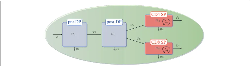
We assume that DN thymocytes differentiate to become pre-selection DP thymocytes with rate (cells/day)φ. We further assume that after the DN stage, thymocyte cell fate is determined by the TCR signal, which a given thymocyte has received. Sinclair et al. used CFSE labeling to show that there is no proliferation at the post-DP stage (see Figure A1 of their manuscript) (21). Stritesky et al. looked at proliferation in the post-DP pool with BrdU label-ing, and found no evidence (26). We have, thus, only included proliferation in the SP thymocyte population (21,26). The three populations,n1,n2, andn3, are involved in the following selection events in the cortex and the medulla (seeFigure 1):
• ∅−→φ n1– flux of DN thymocytes into compartmentn1,
• n1 −ϕ→1 n2– differentiation from pre-DP (n1) to post-DP (n2) thymocytes induced by TCR signal,
• n1−µ→ ∅1 – death by neglect of pre-DP thymocytes due to lack of (or weak) TCR signal,
• n2 −ϕ→2 n3 – differentiation from post-DP (n2) to SP (n3) thymocytes sustained by intermediate TCR signal,
• n2−µ→ ∅2 – apoptosis of post-DP (n2) thymocytes due to strong TCR signal,
• n3 ϕ
3
−→periphery – exit of SP thymocytes (n3) to the periphery (thymic maturation),
• n3−λ→3 2n3– proliferation of SP thymocytes (n3) in the medulla, and
• n3−µ→ ∅3 – apoptosis of SP (n3) thymocytes due to strong TCR signal.
The time evolution of the three populations can be described by the following set of ordinary differential equations (ODEs), which are based on the selection events described above:
dn1
dt =φ−ϕ1n1−µ1n1, dn2
dt =ϕ1n1−ϕ2n2−µ2n2, dn3
dt =ϕ2n2−ϕ3n3−µ3n3+λ3n3.
FIGURE 1 | Thymic development as hypothesized in the first model. The flux,φ, represents the differentiation of DNs into pre-DPs. Pre-DP thymocytes have two fates: further differentiation into the post-DP pool (ϕ1) or death by neglect (µ1). Post-DP
thymocytes have two fates: further differentiation into the SP pool (ϕ2) or death by apoptosis (µ2). Finally, SP thymocytes have three fates: maturation and exit into the periphery (ϕ3), death by apoptosis (µ3), or proliferation (λ3).
We are interested in studying the steady state of these popu-lations, as the experimental data correspond to population cell numbers in the three stages (pre-DP, post-DP, and SP) for a steady state thymus (26). The steady state of the system of equations [equation (1)] is given by:
n∗1 =
φ
ϕ1+µ1 , n ∗ 2 =
n1∗ϕ1
ϕ2+µ2 , n ∗ 3 =
n∗2ϕ2
ϕ3+µ3−λ3 . (2)
This unique steady state exists if and only ifϕ3+µ3−λ3>0, so that we haven∗
3 >0. In order to study the linear stability of the steady state, we calculateA, the Jacobian matrix of equation (1), as follows:
A=
−(ϕ1+µ1) 0 0
ϕ1 −(ϕ2+µ2) 0
0 ϕ2 −(ϕ3+µ3−λ3)
. (3)
A is also the Jacobian matrix at the steady state n∗ =
(n∗1,n ∗ 2,n
∗
3), as the system of ODEs [equation (1)] is linear. The three eigenvalues ofAare given by (as the matrix is lower triangular):
β1= −(ϕ1+µ1), β2= −(ϕ2+µ2), β3= −(ϕ3+µ3−λ3).
Therefore, the steady state [equation (2)] is stable, if and only if,ϕ3+µ3−λ3>0, which is also the condition for its existence. We conclude this section with the analytical solution of the system of ODEs [equation (1)], given initial conditions, which provides the time evolution of the three thymocyte populations:
n1(t)=n∗1+n1(0)e−(ϕ1+µ1)t ,
n2(t)=n∗2+
n1(0) ϕ1
[(ϕ2+µ2)−(ϕ1+µ1)]e
−(ϕ1+µ1)t
+n2(0)e−(ϕ2+µ2)t ,
n3(t)=n∗3+
n1(0) ϕ1
[(ϕ2+µ2)−(ϕ1+µ1)] (4)
× ϕ2
[(ϕ3+µ3−λ3)−(ϕ1+µ1)]e
−(ϕ1+µ1)t
+ n2(0) ϕ3
[(ϕ3+µ3−λ3)−(ϕ2+µ2)]e
−(ϕ2+µ2)t
+n3(0)e−(ϕ3+µ3−λ3)t ,
wheren1(0),n2(0),n3(0) represent the initial conditions for the thymocyte populations. Note that in the late time limit, that is, ift→ +∞andϕ3+µ3−λ3>0, thenn1(t)→n∗1,n2(t)→n∗2 andn3(t)→n3∗, as it is the unique stable steady state.
2.2. A SECOND MODEL OF THYMIC DEVELOPMENT AFTER THE DN STAGE: CD4 AND CD8 SP THYMOCYTES
As described in Section 2.1, the first deterministic model will allow us to calibrate some of the parameters of a more comprehensive model, which we now introduce. We subdivide the SP thymocyte population in two classes: CD4 SP and CD8 SP thymocytes. This is an extension of the model introduced in the previous section, and is motivated by the fact that experimentally, SP thymocytes express either the CD4 or the CD8 co-receptor. We now have four different thymocyte populations to consider:n1, the population of pre-selection DP (double positive) thymocytes,n2, the population of post-selection DP thymocytes,n4, the population of mature CD4+
SP (single positive) thymocytes, andn8, the population of mature CD8+
SP (single positive) thymocytes.
As described in the previous section, we assume that DN thy-mocytes differentiate to become pre-selection DP thythy-mocytes with rate (cells/day) φ, and that after the DN stage, thymocyte cell fate is determined by the TCR signal, which a given thymocyte has received. Thus, the four populations,n1,n2,n4, andn8, with
n3=n4+n8, are involved in the following selection events in the cortex and the medulla (seeFigure 2):
• ∅−→φ n1– flux of DN thymocytes into compartmentn1, • n1 −ϕ→1 n2 – differentiation from pre-DP (n1) to post-DP (n2)
FIGURE 2 | Thymic development as hypothesized in the second model. We assume there is a flux,φ, that represents the differentiation of DNs into pre-DPs. Pre-DP thymocytes have two fates: further differentiation into the post-DP pool (ϕ1) or death by neglect (µ1). Post-DP thymocytes have three
fates: further differentiation into the SP pool as CD4 SPs (ϕ4), or CD8 SPs (ϕ8), or death by apoptosis (µ2). Finally, CD4 or CD8 SP thymocytes have three fates: maturation and exit into the periphery (ξ4) or (ξ8), death by apoptosis (µ4) or (µ8), or proliferation (λ4) or (λ8).
• n1 −µ→ ∅1 – death by neglect of pre-DP thymocytes due to lack of (or weak) TCR signal,
• n2−ϕ→4 n4– differentiation from post-DP (n2) to CD4+SP (n4) sustained by intermediate TCR signal,
• n2−ϕ→8 n8– differentiation from post-DP (n2) to CD8+SP (n8) sustained by intermediate TCR signal,
• n2 µ
2
−→ ∅– apoptosis of post-DP (n2) thymocytes due to strong TCR signal,
• n4 −→ξ4 periphery – exit of CD4+ SP thymocytes (n4) to the periphery (thymic maturation),
• n8 −→ξ8 periphery – exit of CD8+ SP thymocytes (n8) to the periphery (thymic maturation),
• n4−λ→4 2n4– proliferation of CD4+SP thymocytes (n4) in the medulla,
• n8−λ→8 2n8– proliferation of CD8+SP thymocytes (n8) in the medulla,
• n4 µ
4
−→ ∅– apoptosis of CD4+
SP (n4) thymocytes due to strong TCR signal, and
• n8 µ
8
−→ ∅– apoptosis of CD8+
SP (n8) thymocytes due to strong TCR signal.
We assume that all model parameters are positive, that is,µ1,
µ2,µ4,µ8,ϕ1, ϕ2,ϕ4,ϕ8,ξ4,ξ8, φ,λ4, λ8>0, and note that the parameters and thymocyte populations of the first and second model are related by the following equations:
ϕ2=ϕ4+ϕ8, ξ4n4+ξ8n8=ϕ3n3,
µ4n4+µ8n8=µ3n3, λ4n4+λ8n8=λ3n3. (5)
The time evolution of the four populations can be described by the following set of ODEs:
dn1
dt =φ−ϕ1n1−µ1n1, dn2
dt =ϕ1n1−(ϕ4+ϕ8)n2−µ2n2, dn4
dt =ϕ4n2−ξ4n4−µ4n4+λ4n4, dn8
dt =ϕ8n2−ξ8n8−µ8n8+λ8n8.
(6)
We are interested in studying the steady state of these popu-lations, as the experimental data correspond to population cell numbers in the four stages (pre-DP, post-DP, CD4 SP, and CD8 SP) for a steady state thymus (26). The steady state of the system of equations [equation (6)] is given by:
n1∗=
φ
ϕ1+µ1 , n ∗ 2=
n∗1ϕ1
ϕ4+ϕ8+µ2,
n4∗=
n∗2ϕ4
ξ4+µ4−λ4 , n ∗ 8 =
n∗2ϕ8
ξ8+µ8−λ8. (7)
This unique steady state exists if and only ifξ4+µ4−λ4>0 andξ8+µ8−λ8>0, so that we guaranteen∗4 >0 andn∗8 >0. In order to study the linear stability of the steady state, we calculate
B, the Jacobian matrix of equation (6), as follows:
B=
−(ϕ1+µ1) 0 0 0
ϕ1 −(ϕ4+ϕ8+µ2) 0 0
0 ϕ4 −(ξ4+µ4−λ4) 0
0 ϕ8 0 −(ξ8+µ8−λ8)
.
(8)
Bis also the Jacobian at the steady staten∗=(
n∗ 1,n
∗ 2,n
∗ 4,n
∗ 8), as the system of ODEs is linear. The four eigenvalues of B are given by:
β1= −(ϕ1+µ1), β2= −(ϕ4+ϕ8+µ2),
β3= −(ξ4+µ4−λ4), β4= −(ξ8+µ8−λ8).
Therefore, the steady state equation (6) is stable if and only if ξ4+µ4−λ4>0 andξ8+µ8−λ8>0, which is also the condi-tion for its existence. We conclude this seccondi-tion with the analytical solution of the system of ODEs equation (6), given initial condi-tions, which provides the time evolution of the four thymocyte populations:
n1(t)=n1∗+n1(0)e−(ϕ1+µ1)t,
n2(t)=n2∗+
n1(0) ϕ1
[(ϕ4+ϕ8+µ2)−(ϕ1+µ1)]e
−(ϕ1+µ1)t
n4(t)=n4∗+
n1(0) ϕ1
[(ϕ4+ϕ8+µ2)−(ϕ1+µ1)]
× ϕ4+ϕ8
[(ξ4+µ4−λ4)−(ϕ1+µ1)]e
−(ϕ1+µ1)t
+ n2(0) ξ4
[(ξ4+µ4−λ4)−(ϕ4+ϕ8+µ2)]e
−(ϕ4+ϕ8+µ2)t
+n4(0)e−(ξ4+µ4−λ4)t,
n8(t)=n8∗+
n1(0) ϕ1
[(ϕ4+ϕ8+µ2)−(ϕ1+µ1)]
× ϕ4+ϕ8
[(ξ8+µ8−λ8)−(ϕ1+µ1)]e
−(ϕ1+µ1)t
+ n2(0) ξ8
[(ξ8+µ8−λ8)−(ϕ4+ϕ8+µ2)]e
−(ϕ4+ϕ8+µ2)t
+n8(0)e−(ξ8+µ8−λ8)t,
(9) wheren1(0),n2(0),n4(0),n8(0) represent the initial conditions for the thymocyte populations. Note that in the late time limit, that is, ift→ +∞andξ4+µ4−λ4>0 andξ8+µ8−λ8>0, then
n1(t)→n1∗,n2(t)→n2∗,n4(t)→n∗4, andn8(t)→n8∗, as it is the unique stable steady state.
3. RESULTS
3.1. PARAMETER ESTIMATION FOR THE FIRST MODEL (MEANS) In this section, we make use of previously published experimental data (26) that provide thymocyte cell counts for the three subsets considered in the first model: pre-DPs, post-DPs, and SPs. The original experiments have been carried out for two types of mice: wild type mice (Bim+/−) and Bim deficient mice (Bim−/−). In this paper, we will only be considering the wild type experimental results. The data will allow us to provide experimental estimates for the steady state thymocyte cell counts:n∗1,n
∗ 2,n
∗
3. Note that, in order to estimate rates (with units of inverse time), thymo-cyte cell counts are not enough. Thus, we will make use of the additional knowledge provided by experimentally determined res-idence times for each population,τi, withi=1, 2, 3. If we make use
of the model (see Section 2.1), the residence time in compartment
ican be expressed as:
τi=
1 ϕi+µi
, for i∈ {1, 2, 3}.
The experimental data (seeTable 1) correspond to the num-ber of cells (thymocytes) at steady state (26), in each of the thymic compartments considered in the mathematical models (see Sections 2.1 and 2.2), and for eight different mice (j=1, 2,. . ., 8). We have made use of the following average residence times in each compartment (27–29)
τ1=60 h=2.5 days , τ2=16 h=0.67 days ,
τ3=96 h=4 days .
In order to derive estimates for the model parameters, we have carried out the following steps:
1. We make use of the experimentally determined mature SP thy-mocyte flux from the medulla to the periphery, which has been estimated to be 1–4×10⁶cells per day (14,26,30). This flux corresponds to about 1% of thymocytes leaving the thymus every day (30). Given this flux, which we denote byφout,n∗3, and the fact thatφout=ϕ3n∗3, we can obtain an estimate for
ϕ3. We have chosenφoutto be 2.5×10⁶cells per day (14,30). 2. Givenτ3,ϕ3, and the fact thatτ3 = µ31+ϕ3 , we can obtain an
estimate forµ3.
3. Givenτ1,n∗1, and the fact thatn ∗
1 = φ τ1, we can obtain an estimate forφ.
4. We also haven∗
2 =ϕ1τ2n1∗, which, in principle, allows us to estimateϕ1. We make use of linear regression techniques to do so (31,32).
Let us introducea1by the following equation,a1=n
∗
2
n∗
1, and
make use of the experimental data to write:n2∗,i=a n∗,1i+i, fori=1, 2,. . ., 8. Thus, the squared error is given by:
E(a1)= 8
X
i=1
(n2∗,i−a1n1∗,i) 2
.
We minimizeE(a1) with respect toa1, that is dadE1 = 0. Solving fora1, we obtain:
a1=
P8 i=1 n
∗,i
1 n ∗,i
2
P8 i=1(n
∗,i
[image:5.595.46.552.564.705.2]1 ) 2 .
Table 1 | Experimental steady state thymocyte cell counts for the wild type pre-DP, post-DP, CD4 SP, and CD8 SP populations.
Mouse n∗
1(pre-DP) (cells) n
∗
2(post-DP) (cells) n
∗
3(SP) (cells) n
∗
4(SP CD4) (cells) n
∗
8(SP CD8) (cells)
1 82.58×10⁶ 9.30×10⁶ 18.36×10⁶ 13.85×10⁶ 4.51×10⁶
2 142.19×10⁶ 19.94×10⁶ 26.20×10⁶ 18.73×10⁶ 7.46×10⁶
3 89.00×10⁶ 5.98×10⁶ 15.98×10⁶ 11.88×10⁶ 4.10×10⁶
4 29.32×10⁶ 2.09×10⁶ 5.61×10⁶ 4.40×10⁶ 1.21×10⁶
5 29.32×10⁶ 2.09×10⁶ 5.61×10⁶ 4.40×10⁶ 1.21×10⁶
6 51.26×10⁶ 5.93×10⁶ 9.01×10⁶ 6.85×10⁶ 2.16×10⁶
7 64.48×10⁶ 6.81×10⁶ 11.64×10⁶ 9.03×10⁶ 2.61×10⁶ 8 218.94×10⁶ 15.42×10⁶ 40.20×10⁶ 29.46×10⁶ 10.74×10⁶
Mean 88.39×10⁶ 8.45×10⁶ 16.57×10⁶ 12.33×10⁶ 4.25×10⁶
Standard deviation 60.11×10⁶ 5.89×10⁶ 11.05×10⁶ 7.94×10⁶ 3.12×10⁶
Given a1, we can then estimate ϕ1 from the equation
ϕ1= aτ12 .
5. Givenτ1,ϕ1, and the fact thatτ1 = µ1+1ϕ1 , we can obtain an estimate forµ1.
6. We are now left with three remaining parameters:ϕ2,µ2, and
λ3. Given the experimental constraints onτ1,τ2, andτ3, we assume that the average time to proliferate, 1/λ3, cannot be <7 days. Therefore, we consider λ3 to be constrained in the interval [1/7,τ3−1], with time measured in days. We sample equally spaced values forλ3, and for each value, we compute
ϕ2 = n
∗
3(ϕ3+µ3−λ3)
n∗
2 . The ratioa2
= n
∗
3
n∗
2 is computed using the
linear regression method described above (seeFigure 3). In this way, we obtain an estimate forϕ3. We note that thep -values fora1anda2are given by 7.57×10⁻³and 6.85×10⁻³, respectively (both smaller than the significance levelα=0.05). 7. Givenτ2,ϕ2, and the fact thatτ2 = µ2+1ϕ2, we can obtain an
estimate forµ2.
8. From steps 6 and 7 above, we have generated (a table of) val-ues forϕ2andµ2, given a fiducial value forλ3in the interval [1/7,τ3−1]. The mice considered in the experimental study are 5.5–17 weeks old, and their thymus is in steady state (26). Thus, we expect that the parameter values can only be accepted if the corresponding system of ODEs attains steady state by 3 weeks. Therefore, we only accept parameter values which provide thy-mocyte cell counts at time t=21 days that are within one standard deviation from the experimentally determined values (seeTable 1). That is, we impose for the given parameter set that the mathematically predicted valueni(t=21 days) belongs to the intervaln∗
i ±σi, withi=1, 2, 3, and whereni∗is the
(exper-imental) mean number of cells in compartmenti, andσiis the
(experimental) standard deviation in compartmenti, as given inTable 1.
We obtain the following parameter values:
φ=35.350×10⁶cells/day , µ1=0.263 day−1,
µ3=0.099 day−1, ϕ1=0.137 day−1, ϕ3=0.151 day−1,
and
µ2∈ [1.295, 1.443]day−1, ϕ2∈ [0.050, 0.198]day−1,
λ3∈ [0.143, 0.250]day−1.
These parameters imply the following thymic selection rates:
3.1.1. Death rates
9.7×10⁵ cells/h die by neglect in compartment 1 (µ1 n∗ 1), 4.8×10⁵ cells/h die by negative selection in compartment 2 (µ2 n2∗), and 6.9×10⁴ cells/h die by negative selection in compartment 3 (µ3n3∗).
3.1.2. Differentiation rates
[image:6.595.303.550.61.214.2]5.0×10⁵cells/h are positively selected in compartment 1, that is, become post-DP from pre-DP (ϕ1n1∗), 4.4×10⁴cells/h are posi-tively selected in compartment 2, that is, become SP from post-DP (ϕ2 n2∗), and 1.0×10⁵cells/h leave compartment 3 to go to the periphery (ϕ3n∗3).
FIGURE 3 | Linear regression plots for the first model.
3.1.3. Proliferation rate
1.3×10⁵cells/h proliferate in compartment 3 (λ3n∗ 3).
We have also computed the stringency of thymic selection, which we define as given by the ratio:
ϕ3n3∗
φ =6.79% .
Finally, we have computed the (per cell) probability to die, given that the cell is in compartmenti(i=1, 2, 3), as well as the (per cell) probability to proliferate in the medulla. We have obtained:
p1= µ1
µ1+ϕ1
=65.8% , p2= µ2
µ2+ϕ2
=91.7% ,
p3= µ3
µ3+ϕ3+λ3
=22.9% , q3= λ3
µ3+ϕ3+λ3
=42.2% .
3.2. PARAMETER ESTIMATION FOR THE SECOND MODEL (MEANS) In this section, we make use of previously published experimental data (26) that provide thymocyte cell counts for the four subsets considered: pre-DPs, post-DPs, CD4 SPs, and CD8 SPs. We only make use of the experimental data for the wild type mice. The data will allow us to provide experimental estimates for the steady state thymocyte cell counts:n∗1,n
∗ 2,n
∗ 4,n
∗
8. As described in Section 3.1, we also need residence times for each population subset,τi, with i=1, 2, 4, 8. If we make use of the model (see Section 2.2), the residence time in compartmentican be expressed as:
τi =
1 ϕi+µi
, for i∈ {1, 2}, and
τi = 1
ξi+µi
, for i∈ {4, 8}.
Recent experimental data provide support for asymmetric death rates in the CD4 and CD8 SP compartments (21). The estimated death rates for CD4 and CD8 SP thymocytes are1 µ4=0.04 day−1 and µ8=0.11 day−1. We also make use of the estimates derived in Section 3.1 forφ,µ1,µ2,ϕ1, andϕ2. Finally,
the average residence times in each compartment, as described in Section 3.1, are given by:
τ1=60 h=2.5 days , τ2=16 h=0.67 days ,
τ4=96 h=4 days , τ8=96 h=4 days .
In order to derive estimates for the model parameters, we have carried out the following steps:
1. Givenτ4,µ4, and the fact thatτ4 = µ41+ξ4 , we can obtain an estimate forξ4.
2. In the same way, givenτ8,µ8, and the fact thatτ8= µ 1
8+ξ8, we
can obtain an estimate forξ8.
3. We are now left with four remaining parameters:ϕ4,ϕ8,λ4, and
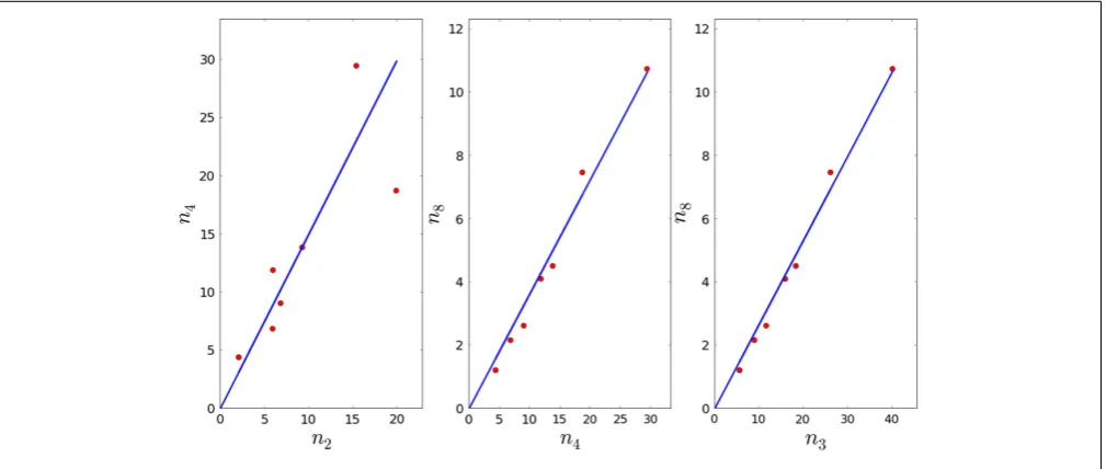
λ8. We know thatϕ2=ϕ4+ϕ8. We sampleϕ4in the interval [0,ϕ2], whereϕ2is the mean value of the interval obtained in Section 2.1, and for each fiducial value forϕ4, we compute the corresponding value forϕ8.
4. Givenτ4,ϕ4, and the fact thatn4∗=
n∗
2ϕ4
τ−1
4 −λ4 , we can compute
the fractiona3 = n
∗
2
n∗
4 by linear regression (seeFigure 4), and
thus obtain an estimate forλ4. Note that we will reject values ofλ4that imply the proliferation time is larger than 7 days (see Section 3.1).
5. In Section 3.1, we obtained an estimate for the mean ofλ3, and we know thatλ4n∗4+λ8n∗8 =λ3n3∗. As before, we can com-pute the fractionsa4 = n
∗
4
n∗
8 anda5
= n
∗
3
n∗
8 by linear regression
(seeFigure 4), and thus obtain an estimate forλ8. Note that we will reject values ofλ8that imply the proliferation time is larger than 7 days (see Section 3.1). We note that thep-values fora3,a4, anda5 are given by 8.43×10⁻³, 3.33×10⁻⁷, and 4.56×10⁻⁸, respectively (smaller than the significance level). 6. From steps 3, 4, and 5 above, we have generated (a table of)
val-ues forϕ8,λ4, andλ8, given a fiducial value forϕ4in the interval
[0,ϕ2]. As discussed in Section 3.1, we only accept parameter values which provide thymocyte cell counts at timet=21 days that are within one standard deviation from the experimentally determined values (seeTable 1).
We obtain the following parameter values:
µ4=0.04 day−1, µ8=0.11 day−1,
ξ4=0.21 day−1, ξ8=0.14 day−1,
and
ϕ4=0.070 day−1, ϕ8=0.054 day−1,
λ4=0.216 day−1, λ8=0.093 day−1.
These parameters imply the following thymic selection rates:
3.2.1. Death rates
2.05×10⁴ cells/h die by negative selection in compartment 4 (µ4 n∗4) and 1.95×10⁴ cells/h die by negative selection in compartment 8 (µ8n8∗).
3.2.2. Differentiation rates
2.50×10⁴cells/h are CD4 positively selected in compartment 2, that is, become CD4 SP from post-DP (ϕ4n∗2), 1.90×10⁴cells/h are CD8 positively selected in compartment 2, that is, become CD8 SP from post-DP (ϕ8n∗2), 1.08×10⁵cells/h leave compart-ment 4 to go to the periphery (ξ4n4∗), and 2.48×10⁴cells/h leave compartment 8 to go to the periphery (ξ8n8∗).
3.2.3. Proliferation rates
11.10×10⁴ cells/h proliferate in compartment 4 (λ4 n∗4) and 1.60×10⁴cells/h proliferate in compartment 8 (λ
[image:7.595.47.552.474.688.2]8n8∗).
We can compute the stringency of thymic selection, defined by the ratio:
ξ4n∗4+ξ8n∗8
φ =8.96% .
We can provide an estimate for the cortical positive selection probabilities, that is the (per post-DP cell) probability to become a CD4 SP or a CD8 SP, and the probability to be negatively selected in the cortex. We have obtained:
s4= ϕ4
µ2+ϕ4+ϕ8
=4.7% , s8= ϕ8
µ2+ϕ4+ϕ8
=3.6% ,
p2= µ2
µ2+ϕ4+ϕ8
=91.7% .
Finally, we have computed the (per cell) probability to die, given that the cell is in compartmenti, as well as the (per cell) probability to proliferate in the medulla. We obtain:
p4= µ4
µ4+ξ4+λ4
=8.6% , q4= λ4
µ4+ξ4+λ4
=46.3% ,
p8= µ8
µ8+ξ8+λ8
=32.1% , q8= λ8
µ8+ξ8+λ8
=27.0% .
These probabilities imply that the probability to exit the thy-mus as a mature CD4 thymocyte (that has already reached the medulla) is given by100−(8.6100+46.3), which is 45.1%, and the proba-bility to exit as a mature CD8 thymocyte (that has already reached the medulla) is given by100−(32.1100+27.0), which is 40.9%.
3.3. SENSITIVITY ANALYSIS
In this section, we explore the sensitivity of the parameters to perturbations in the experimental data. For the first model, the experimental data are given in terms of the following eight quantities:
θ=(τ1,τ2,τ3,φout,a1,a2,n¯3,n¯1),
wherea1,a2are the coefficients of the linear regression ofn
∗
2
n∗
1 and
n∗
3
n∗
2, respectively, and
¯
niis the experimental mean value ofni. We perturb each entry of the vector θ by adding and sub-tracting 10% of its value. Therefore, we now have two values forθi, equal toθi +101θi andθi− 101θi. Consequently, we have
28 sets of θ, which will be used to compute the corresponding model parameters as described in Section 3.1. Parameter val-ues will only be accepted if they provide a stable solution before
t=21 days.
For the second model, the experimental data is given in terms of the following seven quantities:
θ =(τ4,τ8,µ4,µ8,a3,a4,a5),
where a3,a4,a5 are the coefficients of the linear regression of
n∗
2
n∗
4,
n∗
4
n∗
8, and
n∗
3
n∗
8, respectively. We have made use of the means of
[image:8.595.301.551.87.286.2]the following parameters of the first model:φ,ϕ1,µ1,ϕ2,µ2,λ3.
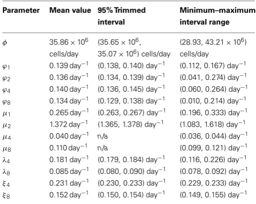
Table 2 | Means, 95% trimmed and minimum–maximum intervals of
the model parameters.
Parameter Mean value 95% Trimmed
interval
Minimum–maximum
interval range
φ 35.86×10⁶
cells/day
(35.65×10⁶,
35.07×10⁶) cells/day
(28.93, 43.21×10⁶)
cells/day
ϕ1 0.139 day−1 (0.138, 0.140) day−1 (0.112, 0.167) day−1 ϕ2 0.136 day−1 (0.134, 0.139) day−1 (0.041, 0.274) day−1 ϕ4 0.140 day−1 (0.136, 0.145) day−1 (0.060, 0.264) day−1 ϕ8 0.134 day−1 (0.129, 0.138) day−1 (0.010, 0.214) day−1 µ1 0.265 day−1 (0.263, 0.267) day−1 (0.196, 0.333) day−1 µ2 1.372 day−1 (1.365, 1.378) day−1 (1.083, 1.618) day−1 µ4 0.040 day−1 n/a (0.036, 0.044) day−1 µ8 0.110 day−1 n/a (0.099, 0.121) day−1 λ4 0.181 day−1 (0.179, 0.184) day−1 (0.116, 0.226) day−1 λ8 0.085 day−1 (0.080, 0.090) day−1 (0.078, 0.092) day−1 ξ4 0.231 day−1 (0.230, 0.233) day−1 (0.229, 0.233) day−1 ξ8 0.152 day−1 (0.150, 0.154) day−1 (0.149, 0.155) day−1
We perturb each entry of the vectorθ as described above. There-fore, we have 27nϕ4 sets ofθ, withnϕ4, the number of different
values considered forϕ4 in the interval (0,ϕ2). Parameter val-ues will only be accepted if they provide a stable solution before
t=21 days.
The results of the sensitivity analysis, with 95% trimmed intervals2and minimum–maximum interval ranges, are given in Table 2.
3.4. VARIABILITY IN THE SELECTION RATES
The (trimmed and minimum–maximum) intervals derived in Section 3.3 allow us to estimate the variability in the different selection rates discussed in Sections 3.1 and 3.2. For example, given variations in the parameters, the corresponding variations in the selection rates can be shown to be:
1pi= 1
(µi+ϕi)2
(ϕi1µi+µi1ϕi) for i=1, 2 , (10)
1p3= 1
(µ3+ϕ3+λ3)2
[(ϕ3+λ3)1µ3+µ31ϕ3+µ31λ3],
(11)
1q3=
1 (µ3+ϕ3+λ3)2
[λ31µ3+λ31ϕ3+(µ3+ϕ3)1λ3],
(12)
1si= 1
(µ2+ϕi+ϕj)2
[ϕi1µ2+ϕi1ϕj
+(µ2+ϕj)1ϕi] for i=4,j=8 or i=8,j=4 ,
(13)
1pi= 1
(µi+ξi+λi)2
[µi1ξi+µi1λi
+(ξi+λi)1µi] for i=4, 8 , (14)
2We define the 95% trimmed interval to be the result of the sensitivity analysis after
1qi= 1
(µi+ξi+λi)2
[λi1ξi+λi1µi
+(ξi+µi)1λi] for i=4, 8 . (15)
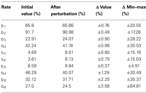
We present inTable 3the variability of the selection rates.
4. DISCUSSION
We have brought together experimental data with a mathemati-cal compartment model [similar to other progression models of CD4 and CD8 T cell development (13,14,18,21,33)] to provide estimates for the selection events that take place in the thymus. We have made use of a range of experimental data: (i) steady state thymocyte cell counts (26), mean residence times in each com-partment (27–29), murine thymic export rate (14,26,30), and recently reported asymmetric death rates for the CD4 SP and CD8 SP thymocytes (21). Our preliminary results support the unex-pectedly high death rate in the post-DP thymocyte population observed in Ref. (21). We note that our approach is unrelated to that of Sinclair et al. both experimentally and mathematically (21). This rate,µ2, has been estimated to be at least an order of magnitude larger than any of the other death rates in the pre-DP, CD4 SP, or CD8 SP pools (seeTable 2). In terms of selection rates, our analysis yields the following: pre-selection thymocytes (pre-DPs) have a 65.8% probability of dying by neglect in the cortex, and a 34.2% probability of becoming post-selection thy-mocytes (post-DPs). At the post-selection stage, post-DPs have a 91.7% probability of dying by negative selection (apoptosis) in the cortex, a 4.7% probability of becoming CD4 SPs, and a 3.6% probability of becoming CD8 SPs. In the medulla, CD4 SPs have an 8.6% probability of dying by negative selection (apoptosis), whereas CD8 SPs have a 32.1% probability of dying by negative selection. CD4 SPs have a 45.1% probability of exiting the thymus and reaching the periphery as mature thymocytes, whereas that probability for CD8 SPs is only 40.9%. Finally, the data supports some level of cellular proliferation in the medulla, with CD4 SPs having a 46.3% probability of proliferation and CD8 SPs a 27% probability.
[image:9.595.301.550.85.243.2]Earlier work by Mehr and collaborators combined experi-mental and theoretical approaches to estimate thymic selection rates (13,33), neglected death rates in the medulla, but consid-ered potential feedback from mature T cells. In agreement with these authors, our results indicate that thymocyte death is high-est at the post-DP stage. However, as death in the medulla had been neglected, these authors concluded that the CD4:CD8 ratio in SP thymocytes is determined by the differentiation rates. In this paper, we have made use of CD4 and CD8, or medullary, death rates, which allowed us to directly compare cortical (DP) to medullary (SP) death rates. Furthermore, our approach allowed us to conclude that medullary, or SP, death was due to negative selection, as it was rescued by Bim deficiency (26). Sinclair et al. also recently addressed the temporal dynamics of thymic selection using an unrelated approach (both experimentally and mathe-matically) (21). While their experimental approach did not allow them to distinguish death by negative selection from death by other mechanisms, their overall finding was consistent with ours, that thymocyte death is highest at the post-DP stage.
Table 3 | Selection rate values (initial and after perturbation) and their
variability intervals.
Rate Initial
value (%)
After
perturbation (%)
1Value (%)
1Min–max (%)
p1 65.8 65.66 ±0.76 ±20.55
p2 91.7 90.98 ±0.49 ±17.28
p3 22.91 24.07 ±0.90 ±28.22
q3 42.24 41.74 ±0.99 ±30.53
s4 4.69 8.51 ±0.80 ±15.16
s8 3.61 8.13 ±0.79 ±15.03
p4 8.59 8.84 ±0.37 ±4.91
q4 46.29 40.07 ±1.29 ±20.49
p8 32.12 31.71 ±2.25 ±35.37
q8 27.0 24.5 ±3.58 ±64.81
Further attempts to quantify thymic selection rates making use of mathematical models also include those of Faro et al. (12). The mathematical model developed by Faro and collaborators does not include time dynamics, but describes the relationship between the number of selecting ligands and the probability of selection of a given thymocyte. Thomas-Vaslin et al. (14) obtained esti-mates of thymic selection rates, using an experimental procedure that temporarily blocks thymic output and a mathematical model in which rates of transit from compartment to compartment depend on the number of cell divisions. Their model can capture the thymic “conveyor belt” (34,35) scheme, but requires more differential equations and more parameters than equation (6). Despite the differences between their theoretical and experimen-tal models and ours, similar estimates for thymic selection rates are found. For example, we estimate that 1.2 million post-DP become CD4 SP thymocytes per day and 0.5 million post-DP become CD8 SP thymocytes per day; their estimates are 0.9 and 0.2 million, respectively. Finally, we estimate that 2.6 million CD4 SP thymocytes per day and 0.6 million CD8 SP thymocytes per day exit the thymus. Their estimates are 2.4 and 0.5 million, respectively.
Section 3.2): (i) the CD4:CD8 ratio of positive selection in the post-DP pool (differentiation from post-DP to either CD4 SP or CD8 SP) is given by ϕ4
ϕ8 ≈5 : 4, (ii) the CD4:CD8 ratio in the SP
pool is given byn
∗
4
n∗
8
≈3 : 1, and (iii) the CD4:CD8 ratio of
posi-tive selection in the SP pool (differentiation from SP to peripheral early thymic emigrants) is given by ξ4n∗4
ξ8n∗8
≈ 4 : 1. Our
observa-tions indicate that the CD4 bias is progressively established, as the thymocytes mature from the post-DP stage until the exit of the SP stage to migrate to the periphery.
Our mathematical analysis has also allowed us to estimate the stringency of thymic selection, defined by:
σ= ξ4n ∗ 4+ξ8n∗8
φ =8.96% ,
that is, the ratio between the number of thymocytes per unit time that exit the thymus and the number of thymocytes per unit time that enter the pre-DP stage. The sensitivity analysis described in Section 3.3 allows us to provide a value of 1σ=0.2%, where we have made use of the minimum–maximum interval ranges (see fourth column ofTable 2). A different measure of stringency could be based on the probability of a cell surviving the maturation process. In our notation, this would correspond to the following:
(1−p1)×(1−p2)×(1−p3)=2.19% .
We note that this measure of stringency is the probability of not dying in any of the three compartments considered in the model (pre-DP, post-DP, and SP). As discussed in Appendix A.1, and given that in the SP pool, thymocytes may proliferate, there is a need to consider this special case. Our estimates suggest that a population of 103pre-DP thymocytes will yield 69 CD4 and 25 CD8 SP thymocytes that leave the medulla to get incorporated into the peripheral naive T cell pool (see details in Appendix A.1).
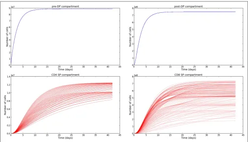
[image:10.595.45.550.382.671.2]The sensitivity analysis (see Section 3.3) and the variability of the selection rates derived from it (see Section 3.4) give us the con-fidence to conclude, that our parameter estimation is robust. We are aware that the experimental data we have made use of [steady state thymocyte cell counts (26)] do not provide the exquisite time resolution described in Ref. (21). However, the supporting math-ematical model described in Section 2.2, allows us to obtain the time evolution of the thymocyte populations, once the parameters have been estimated. InFigure 5, we plot the time evolution of the total number of cells in each compartment of the mathemat-ical model: pre-DP, post-DP, CD4 SP, and CD8 SP thymocytes. We start with no cells at time zero,ni(t=0)=0 fori=1, 2, 4, 8. Trajectories have been plotted for a period of 6 weeks and have been computed for every permutation of the parameter set pre-sented inTable 2. The subset of parameters shared with the simple model (φ,ϕ1,µ1,µ2), were fixed at their mean values. Thus, 548 distinct parameter sets were generated. The system of equations (6) was solved using a fourth order Runge–Kutta method (Python source code).
The approaches introduced in this paper have shed some light on the probabilities and timescales that characterize cellu-lar fate in the thymus after the DN stage. We plan to generalize the mathematical model introduced here, making use of experi-mental data for the strength of TCR binding in Nur77GFP mice (26), to investigate issues such as the death rate in the post-DP pool and the CD4:CD8 ratio. Our model assumes that all progenitors in a particular pool behave with identical kinetics, i.e., move through the various stages of selection at the same rate. Future model refinements will come from consideration of the heterogeneity of the pools, which are known to include cells that will become iNKT cells, regulatory T cells, and intra-epithelial lymphocytes (2). It is also possible that progenitors of the same general class move through the selection process with different kinetics (34). The models introduced here can serve as a first step to study human thymic selection, although com-prehensive data on human thymic subsets, their sizes, and res-idence times are not yet available. It would be of great interest to apply the model to data on thymic subsets and cellularity in children, keeping in mind that residence times of human sub-sets may differ from murine ones (38). Finally, we note that we have not mentioned the relevance of cytokines, such as IL-7, during thymic development. Some differences have already been described for the role of IL-7R in human versus mouse T cell development (38, 39). We hope in the near future to combine mechanistic mathematical models of IL-7 and IL-7R (40) with the T cell development model introduced here to address these issues.
ACKNOWLEDGMENTS
We thank Ed Palmer, Robin Callard, Andy Yates, and Ben Sed-don for helpful discussions, and Andy Yates and Ben SedSed-don for allowing us to make use of their mathematical estimates for µ4 and µ8. Grant Lythe and Carmen Molina-París thank Bill Hlavacek, Ruy Ribeiro, and Alan Perelson (Los Alamos National Laboratory) for their hospitality. This work was supported by a BBSRC Research Development Fellowship BB/G023395/1 (to Car-men Molina-París), an FP7 IRSES INDOEUROPEAN-MATHDS Network PIRSES-GA-2012-317893 (to Grant Lythe and Carmen Molina-París), and National Institutes of Health Grants R37 AI39560 (to Kristin A. Hogquist) and F32 AI100346 (to Gretta L. Stritesky). Maria Sawicka, Joseph Reynolds, Niloufar Abourashchi, Grant Lythe, and Carmen Molina-París acknowledge the hospi-tality of the Max Planck Institute for the Physics of Complex Systems, Dresden, and the International Centre for Mathemati-cal Sciences, Edinburgh, where part of this work was discussed and presented.
REFERENCES
1. Anderson G, Lane P, Jenkinson E. Generating intrathymic microenviron-ments to establish T-cell tolerance.Nat Rev Immunol (2007)7(12):954–63. doi:10.1038/nri2187
2. Stritesky GL, Jameson SC, Hogquist KA. Selection of self-reactive T cells in the thymus.Annu Rev Immunol(2012)30:95. doi:10.1146/annurev-immunol-020711-075035
3. Palmer E. Negative selection: clearing out the bad apples from the T-cell reper-toire.Nat Rev Immunol(2003)3(5):383–91. doi:10.1038/nri1085
4. Jameson S, Hogquist K, Bevan M. Positive selection of thymocytes.Annu Rev Immunol(1995)13(1):93–126. doi:10.1146/annurev.iy.13.040195.000521 5. Werlen G, Hausmann B, Naeher D, Palmer E. Signaling life and death in the
thy-mus: timing is everything.Science(2003)299(5614):1859. doi:10.1126/science. 1067833
6. Petrie H, Zúñiga-Pflücker J. Zoned out: functional mapping of stromal sig-naling microenvironments in the thymus. Immunology (2007) 25(1):649. doi:10.1146/annurev.immunol.23.021704.115715
7. Zúñiga-Pflücker JC. When three negatives made a positive influence in defin-ing four early steps in T cell development.J Immunol(2012)189(9):4201–2. doi:10.4049/jimmunol.1202553
8. Takada K, Ohigashi I, Kasai M, Nakase H, Takahama Y. Development and func-tion of cortical thymic epithelial cells.Curr Top Microbiol Immunol (2013) 373:1–17.
9. Singer A, Adoro S, Park J. Lineage fate and intense debate: myths, models and mechanisms of CD4-versus CD8-lineage choice.Nat Rev Immunol(2008) 8(10):788–801. doi:10.1038/nri2416
10. Anderson MS, Su MA. Aire and T cell development.Curr Opin Immunol(2011) 23(2):198–206. doi:10.1016/j.coi.2010.11.007
11. Klein L. Dead man walking: how thymocytes scan the medulla.Nat Immunol (2009)10(8):809–11. doi:10.1038/ni0809-809
12. Faro J, Velasco S, Gonzalez-Fernandez A, Bandeira A. The impact of thymic antigen diversity on the size of the selected T cell repertoire.J Immunol(2004) 172(4):2247.
13. Mehr R, Globerson A, Perelson A. Modeling positive and negative selection and differentiation processes in the thymus.J Theor Biol(1995)175(1):103–26. doi:10.1006/jtbi.1995.0124
14. Thomas-Vaslin V, Altes H, de Boer R, Klatzmann D. Comprehensive assessment and mathematical modeling of T cell population dynamics and homeostasis. J Immunol(2008)180(4):2240.
15. Souza-e Silva H, Savino W, Feijóo R, Vasconcelos A. A cellular automata-based mathematical model for thymocyte development.PLoS One(2009)4(12):e8233. doi:10.1371/journal.pone.0008233
16. Efroni S, Harel D, Cohen I. Emergent dynamics of thymocyte development and lineage determination.PLoS Comput Biol(2007)3(1):e13. doi:10.1371/journal. pcbi.0030013
17. Müller V, Bonhoeffer S. Quantitative constraints on the scope of negative selec-tion.Trends Immunol(2003)24(3):132–5. doi:10.1016/S1471-4906(03)00028-0 18. Detours V, Mehr R, Perelson A. A quantitative theory of affinity-driven T cell repertoire selection.J Theor Biol(1999)200(4):389–403. doi:10.1006/jtbi.1999. 1003
19. Prasad A, Zikherman J, Das J, Roose J, Weiss A, Chakraborty A. Origin of the sharp boundary that discriminates positive and negative selection of thymocytes. Proc Natl Acad Sci U S A(2009)106(2):528. doi:10.1073/pnas.0805981105 20. Ribeiro RM, Perelson AS. Determining thymic output quantitatively: using
models to interpret experimental T-cell receptor excision circle (Trec) data. Immunol Rev(2007)216(1):21–34.
21. Sinclair C, Bains I, Yates AJ, Seddon B. Asymmetric thymocyte death underlies the CD4:CD8 T-cell ratio in the adaptive immune system.Proc Natl Acad Sci U S A(2013)110(31):E2905–14. doi:10.1073/pnas.1304859110
22. Surh CD, Sprent J. T-cell apoptosis detected in situ during positive and negative selection in the thymus.Nature(1994)372(6501):100–3. doi:10.1038/372100a0 23. Laufer TM, DeKoning J, Markowitz JS, Lo D, Glimcher LH. Unopposed positive selection and autoreactivity in mice expressing class II MHC only on thymic cortex.Nature(1996)383(6595):81–5. doi:10.1038/383081a0
24. van Meerwijk JP, Marguerat S, Lees RK, Germain RN, Fowlkes B, MacDonald HR. Quantitative impact of thymic clonal deletion on the T cell repertoire.J Exp Med(1997)185(3):377–84. doi:10.1084/jem.185.3.377
25. Merkenschlager M, Graf D, Lovatt M, Bommhardt U, Zamoyska R, Fisher AG. How many thymocytes audition for selection?J Exp Med(1997)186(7):1149–58. doi:10.1084/jem.186.7.1149
28. Saini M, Sinclair C, Marshall D, Tolaini M, Sakaguchi S, Seddon B. Regulation of Zap70 expression during thymocyte development enables temporal separation of CD4 and CD8 repertoire selection at different signaling thresholds.Sci Signal (2010)3(114):ra23. doi:10.1126/scisignal.2000702
29. McCaughtry TM, Wilken MS, Hogquist KA. Thymic emigration revisited.J Exp Med(2007)204(11):2513–20. doi:10.1084/jem.20070601
30. Scollay RG, Butcher EC, Weissman IL. Thymus cell migration: quantitative aspects of cellular traffic from the thymus to the periphery in mice. Eur J Immunol(1980)10(3):210–8. doi:10.1002/eji.1830100310
31. Kenney JF, Keeping ES.Mathematics of Statistics: Part One. Princeton: van Nos-trand (1954).
32. Kenney JF, Keeping ES.Mathematics of Statistics: Part Two. Princeton: van Nos-trand (1962).
33. Mehr R, Perelson A, Fridkis-Hareli M, Globerson A. Feedback regulation of T cell development in the thymus. J Theor Biol (1996)181(2):157–67. doi:10.1006/jtbi.1996.0122
34. Scollay R, Godfrey D. Thymic emigration: conveyor belts or lucky dips?Immunol Today(1995)16(6):268–73. doi:10.1016/0167-5699(95)80179-0
35. Tough DF, Sprent J. Thymic emigration: conveyor belts or lucky dips?Immunol Today(1995)16(6):273–4. doi:10.1016/0167-5699(95)80180-4
36. Sim B-C, Aftahi N, Reilly C, Bogen B, Schwartz RH, Gascoigne NR, et al. Thymic skewing of the CD4/CD8 ratio maps with the T-cell receptorα-chain locus.Curr Biol(1998)8(12):701–S3. doi:10.1016/S0960-9822(98)70276-3
37. Boursalian TE, Golob J, Soper DM, Cooper CJ, Fink PJ. Continued matura-tion of thymic emigrants in the periphery.Nat Immunol(2004)5(4):418–25. doi:10.1038/ni1049
38. Spits H. Development ofαβT cells in the human thymus.Nat Rev Immunol (2002)2(10):760–72. doi:10.1038/nri913
39. Marino JH, Tan C, Taylor AA, Bentley C, Van De Wiele CJ, Ranne R, et al. Differ-ential IL-7 responses in developing human thymocytes.Hum Immunol(2010) 71(4):329–33. doi:10.1016/j.humimm.2010.01.009
40. Molina-París C, Reynolds J, Lythe G, Coles MC. Mathematical model of naive t cell division and survival il-7 thresholds.Front Immunol(2013)4:434. doi:10.3389/fimmu.2013.00434
41. Allen LJS.An Introduction to Stochastic Processes with Applications to Biology. New Jersey: Pearson Education (2003).
Conflict of Interest Statement:The authors declare that the research was conducted in the absence of any commercial or financial relationships that could be construed as a potential conflict of interest.
Received: 11 September 2013; accepted: 15 January 2014; published online: 14 February 2014.
Citation: Sawicka M, Stritesky GL, Reynolds J, Abourashchi N, Lythe G, Molina-París C and Hogquist KA (2014) From pre-DP, post-DP, SP4, and SP8 thymocyte cell counts to a dynamical model of cortical and medullary selection. Front. Immunol.5:19. doi: 10.3389/fimmu.2014.00019
This article was submitted to T Cell Biology, a section of the journal Frontiers in Immunology.
APPENDIX
A.1. STRINGENCY OF THYMIC SELECTION: A STOCHASTIC MODEL In this section, we present the details that allow us to compute the stringency of thymic selection for the mathematical model considered in Section 2.2.
Let us assume that at timet=0, there exists a single T cell in a given compartment. In our case, the compartment can be the pre-DP, post-DP, or SP (either CD4 SP or CD8 SP) stages. The cell, at any time, may die (with rate,µ), divide (with rate,λ), and produce two daughter cells, or leave the compartment (with rate, ξ) to enter a different compartment. The waiting times for each event are assumed to be exponentially distributed, and daughter cells are assumed to behave identically to the initial single cell. We introduce the bivariate Markov process {X(t),Y(t)}t≥0, where
X(t) is the number of cells in the compartment at timet, andY(t) is the number of cells which have left the compartment (to enter a different compartment). Our aim is to calculate the expected number of cells (and variance) that leave the compartment.
State probabilities for the Markov process are defined as follows (41)
p(x,y)(t)=Prob{X(t)=x,Y(t)=y|X(0)=1,Y(0)=0},
(A1) and transition probabilities for this process are defined as fol-lows (41)
p(w,z),(x,y)(1t)=Prob{X(t+1t)=w, Y(t+1t)=z|X(t)=x,Y(t)=y}
=
λx1t+o(1t), ifw=x+1,z=y, µx1t+o(1t), ifw=x−1,z=y, ξx1t +o(1t), ifw=x−1,z=y+1 , 1−(λ+µ+ξ)x1t+o(1t), ifw=x,z=y,
o(1t), ifw,zotherwise . (A2) The Kolmogorov (or master) equation for this process is given by (41)
dp(x,y)(t)
dt =λ (x−1)p(x−1,y)(t)+µ (x+1)p(x+1,y)(t)
+ξ (x+1)p(x+1,y−1)(t)−(λ+µ+ξ)x p(x,y)(t).
(A3)
LetmX(t) be the expected number of cells in the compart-ment under consideration, and mY(t) be the expected number of cells which have left the compartment. Similarly, letmXX(t) be the expectation of the random variableX(t)2,mXY(t) be the expectation of the random variableX(t)Y(t), andmYY(t) be the expectation of the random variableY(t)2. Then, making use of the probability generating function technique (41), we derive the time evolution for the first two moments of the system:
dmX(t)
dt =(λ−µ−ξ)mX(t), (A4)
dmY(t)
dt =ξmX(t), (A5)
dmXX(t)
dt =2(λ−µ−ξ)mXX(t)+(λ−µ−ξ)mX(t), (A6)
dmXY(t)
dt =(λ−µ−ξ)mXY(t)+ξ[mXX(t)−mX(t)], (A7)
dmYY(t)
dt =ξ[2mXY(t)+mX(t)]. (A8)
Given that we start with a single cell, the expected number of cells at timetis given by
mX(t)=e(λ−µ−ξ)t. (A9)
Under the restrictionλ < µ+ξ, the expected number of cells tends to zero ast→ +∞. This implies that all cells from the single T cell progenitor either die or leave the compartment for suffi-ciently large times. The expected number of cells which leave the compartment is given by
mY(t)= ξ
µ+ξ−λ
h
1−e(λ−µ−ξ)t
i
. (A10)
Ast→ +∞, the expected number of cells to leave the compart-ment can be shown to be
lim
t→+∞mY(t)=
ξ
µ+ξ−λ. (A11)
We now solve the remaining ODEs equations (A6–A8), to find
mYY(t)= 2λξ
2
(λ−µ−ξ)3
1 2e
2(λ−µ−ξ)t−e(λ−µ−ξ)t
− 4λξ
2
(λ−µ−ξ)2
t− 1
λ−µ−ξ
e(λ−µ−ξ)t
+ ξ
λ−µ−ξe
(λ−µ−ξ)t − 2λξ2 (λ−µ−ξ)3
− ξ
λ−µ−ξ . (A12)
It, therefore, follows that the random variable Y(t), which represents the number of cells leaving the compartment under consideration, has the following variance (in the limitt→ +∞)
σ2
Y =tlim→∞
mYY(t)−mY(t)2
= 2λξ
2
(µ+ξ−λ)3 +
ξ µ+ξ−λ
− ξ
2
(µ+ξ−λ)2 . (A13)
A.2. STRINGENCY OF THYMIC SELECTION IN THE FOUR COMPARTMENT MODEL
The previous example can easily (but laboriously) be extended to the mathematical model introduced in Section 2.2.
compartment (pre-DP, post-DP, SP CD4, and SP CD8) are left for the reader to derive. When counting the number of CD4+
T cells leaving the thymus, the moment generating function satisfies the following partial differential equation
∂M ∂t =µ1(e
−θ1
−1)∂M ∂θ1
+ϕ1(e−θ1eθ2−1)∂M
∂θ1
+(µ2+ϕ8)(e−θ2−1)∂M
∂θ2
+ϕ4(e−θ2eθ4−1)∂M
∂θ2
+µ4(e−θ4−1)∂M
∂θ4
+λ4(eθ4−1)∂M
∂θ4
+ξ4(e−θ4eθ8−1)∂M
∂θ4
. (A14)
The symmetry of the mathematical model implies that an equivalent equation for the number of CD8+
T cells leaving the thymus can be obtained by interchanging the indexes 4 and 8. For our derived parameter set, the previous equation allows us to conclude that the expected number of CD4+
T cells, a single thy-mocyte in the pre-DP compartment produces, is 0.069 (standard deviation 0.96), whereas the expected number of CD8+
T cells which leave the thymus is 0.025 (standard deviation 0.59).
To put this into perspective, a population of 103 pre-DP thy-mocytes is expected to produce 69 CD4+
T cells which leave the thymus (standard deviation 66), and 25 CD8+
T cells (standard deviation 41). More generally, a population ofN pre-DP thymo-cytes is expected to produce 0.069N CD4+
T cells and 0.025N