Fault Tolerant Computation of Hyperbolic Partial Differential Equations with the Sparse Grid Combination Technique

(1)

Fault Tolerant Computation of

Hyperbolic Partial Differential Equations

with the Sparse Grid Combination

Technique

Brendan Harding

August 2015

(revised April 2016)

(2)

(3)

Declaration

Some of the work in this thesis has been published jointly with others, see for example [67, 68, 5, 120, 69, 3, 66, 80, 79], however my own contribution to these works has been the development and analysis of the fault tolerant combination technique which is the focus of this thesis. The work in this thesis is my own except where otherwise stated.

(4)

(5)

Acknowledgements

I would like to acknowledge my supervisor Markus Hegland and the other mem-bers of my supervisory panel Michael Barnsley and Steve Roberts. I had the priv-ilege of being able to contribute to a collaborative project (project LP110200410 under the Australian Research Council’s Linkage Projects funding scheme) and would like to thank the other members of the project for the many interesting dis-cussions. Specifically thanks to Peter Strazdins, Mohsin Ali, Linda Stals, Alistair Rendell and Jay Larson. Fujitsu Laboratories of Europe was the collaborative partner in this project and I would also like to thank Ross Nobes, James Southern and Nick Wilson for the interactions I had with them throughout the project and for hosting me for 6 weeks in the Hayes office in 2014. I was also fortunate to in-teract with many members of the sparse grid and high dimensional approximation communities. I am very grateful having had the opportunity to share and discuss ideas with the many members of these communities, particularly those who re-side in Germany through my short stays in Munich and the many visitors of the Mathematical Sciences Institute. Many computations relating to this work were performed on Raijin, the peak system at the NCI Facility in Canberra, Australia, which is supported by the Australian Commonwealth Government. Finally, a big thank you to my family and friends for their support and encouragement throughout my studies.

(6)

(7)

Abstract

As the computing power of supercomputers continues to increase exponentially the mean time between failures (mtbf) is decreasing. Checkpoint-restart has

historically been the method of choice for recovering from failures. However, such methods become increasingly inefficient as the time required to complete a checkpoint-restart cycle approaches the mtbf. There is therefore a need to

explore different ways of making computations fault tolerant. This thesis studies generalisations of the sparse grid combination technique with the goal of develop-ing and analysdevelop-ing a holistic approach to the fault tolerant computation of partial differential equations (pdes).

Sparse grids allow one to reduce the computational complexity of high di-mensional problems with only small loss of accuracy. A drawback is the need to perform computations with a hierarchical basis rather than a traditional nodal basis. We survey classical error estimates for sparse grid interpolation and ex-tend results to functions which are non-zero on the boundary. The combination technique approximates sparse grid solutions via a sum of many coarse approx-imations which need not be computed with a hierarchical basis. Study of the combination technique often assumes that approximations satisfy an error split-ting formula. We adapt classical error splitsplit-ting results to our slightly different convention of combination level.

Literature on the application of the combination technique to hyperbolicpdes

is scarce, particularly when solved with explicit finite difference methods. We show a particular family of finite difference discretisations for the advection equa-tion solved via the method of lines has soluequa-tions which satisfy an error splitting formula. As a consequence, classical error splitting based estimates are read-ily applied to finite difference solutions of many hyperbolic pdes. Our analysis

also reveals how repeated combinations throughout the computation leads to a reduction in approximation error.

Generalisations of the combination technique are studied and developed at

(8)

depth. The truncated combination technique is a modification of the classical method used in practical applications and we provide analogues of classical error estimates. Adaptive sparse grids are then studied via a lattice framework. A detailed examination reveals many results regarding combination coefficients and extensions of classical error estimates. The framework is also applied to the study of extrapolation formula. These extensions of the combination technique provide the foundations for the development of the general coefficient problem. Solutions to this problem allow one to combine any collection of coarse approximations on nested grids.

(9)

Chapter 1 Faults in High Performance

Computing

In this thesis we are concerned with the development of fault tolerant algorithms for solving pdes. In order to motivate this we discuss the occurrence of faults

in current and future computer systems. Questions of importance are why do faults occur, how often do faults occur, what types of faults occur, and how do faults affect computations? After surveying several articles which attempt to answer these questions in Section 1.1 we start to develop several different models of faults. As faults are random in nature these models are necessarily stochastic. In Section 1.2 fault models for a single processor are discussed. As a high performance computer is essentially collection of electrical components working in parallel this will be a fundamental building block of system models which are considered in Section 1.3. Lastly, in Section 1.4 we apply fault models to some simple calculations in a parallel environment, we review the estimation of the optimal checkpoint frequency for checkpoint-restart based routines and we study the problem of simulating faults.

1.1 Motivation and background

1.1.1 Faults in HPCs

In the 1940s and 1950s the first all-electric computers were constructed using vacuum tubes as the electric switches that performed bitwise operations. The most notable computers of the time consisted of several thousand vacuum tubes, the ENIAC (Electronic Numerical Integrator And Computer) had over 17 000.

(12)

There were several issues with vacuum tubes at the time including size, cost, and a relatively short mean time to failure. Now it is important to clarify what we mean by relatively short life span. A long-life vacuum tube at the time had a life expectancy in the order of O(5 000) hours [97] (some specially designed tubes in the 1950s had much more) which was reasonable given the manufacturing processes of the time. However, having several thousand such vacuum tubes operating at once it was observed that tubes would fail and need to be replaced at a frequency in the order of days. A notable example is the ENIAC for which it was stated that a tube failed roughly every 2 days [2].

Since the advent of transistors and their incorporation into integrated circuits it has been possible to have large numbers of electric switches on a single com-ponent. This soon lead to components in the early 1970s whose life expectancy was of a similar magnitude as the vacuum tube but could do the same amount of work as computers containing thousands of such tubes. This lead to a significant improvement in the reliability of computers vs computing power. With improved photolithography techniques allowing for ever smaller transistors to be etched into semiconductors the trend continued allowing what is now in the order of bil-lions of transistors on a single electrical component whose lifetime exceeds that of the average vacuum tubes in the first all-electric computers. Modern CPUs are so reliable that failures in a modern computer are more likely to have root cause in other components like the power supply, hard drives, cooling systems, etc.

(13)

103 104 105 106 107 100

101 102

103

# sockets

SMTTI

(hours)

R = 0.99999

[image:13.595.217.422.99.267.2]

R = 0.999999

Figure 1.1: System mean time to interrupt (SMTTI) versus the number of sockets N

for different one-hour socket reliabilitiesR= 0.999 99andR= 0.999 999[26]. The plot is of the estimate SM T T I = 1/(1−RN₎ _{which is flawed in that the limit is} ₁ _{hour as} N → ∞ with0< R <1.

that is where the number of components is similar in magnitude to the expected life time of these components (in hours). Thus we would expect that reliability will again become an issue for high performance computing. Whilst this discus-sion so far has been somewhat anecdotal, several recent studies and surveys have observed this trend.

In recent years there have been several survey articles predicting a decreasing mean time between failure in high performance computers, see for example [26, 117, 27, 105]. The major contributing factor for this trend is typically identified to be increasing system sizes. As the clock rate of individual cores is no longer increasing in significant amounts, higher performance is achieved primarily by increasing the number of cores. Although this is partially offset by increasing numbers of cores per socket, the largest systems contain an increasing numbers

of components. As one would reasonably expect twice as many components

to fail twice as often, the increases in number of components is the primary driver of decreasing mtbf (mean time between failures). More precisely, if a

single component has a (constant) failure rateF, that is in any given hour it has probability F of failing, then it has probability 1−F of not failing in a given hour. It follows that forN identical components with the same (constant) failure rate the probability that none fail within any given hour is (1−F)N_{, thus at}

least one fails with probability 1−(1−F)N_{. For small} _F _(and _{N <<}₁_/F_{) this}

(14)

demonstrates the decrease in system mean time to interrupt (SMTTI) for some different levels of reliability R = 1−F based on this simple model. This trend was observed by Schroeder and Gibson in their study of computers at LANL (Los Alamos National Laboratory) which found that the rate of failure was roughly proportional to the number of nodes in each system [116].

A second contributing factor is that the reliability of individual components is likely to decrease as feature size becomes smaller [33, 28] and chips become more heterogeneous due to increased integration. The reliability of components is also closely linked with energy consumption. For example, typically noise in the_cpuis addressed by error detection and correction mechanisms built into the hardware. However this consumes a significant portion of the total energy. As improving energy efficiency is also one of the big challenges for exascale computing [37], it seems unlikely that increased _cpu noise caused by decreasing feature size can be entirely addressed by changes in hardware if the energy target of 100 MW for an exascale computer is to be achieved. Compute nodes are also becoming increasingly complex particularly as general purpose graphics processing units and other accelerators become integrated into more systems. Similarly to the entire _hpc system, the reliability of individual nodes will likely decrease as more components are added to them.

These arguments would indicate that hardware is the primary source of faults in _hpc’s, that is that failures in the system occur when a physical component breaks down. Faults are typically classified into one of three categories [101]:

• permanent fault: a component may completely break down such that it no longer functions or produces incorrect results,

• transient fault: a component may temporarily have reduced performance or produce incorrect results,

• intermittent faults: a component oscillates between correct and incorrect operation.

(15)

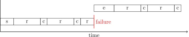
time

s r c r c r _failure

[image:15.595.120.520.107.185.2]

e r c r c

Figure 1.2: Schematic of a simple checkpoint restart implementation. Block ‘s’ is for program startup, ‘r’ is main program execution, ‘c’ is for writing checkpoints, ‘e’ is the restart of the application and loading of the previous checkpoint.

to hardware faults is not so clear as different studies in the literature give very different results. The recent study of Schroeder and Gibson showed that hardware is the most common cause followed by software. However a other studies [102, 93, 55] have indicated that software was the largest cause of failures. In this thesis we are not particularly concerned with the root cause but it is clear that more systems need to be studied if we are to better understand the causes and effects of faults in a system.

In most current systems, regardless of the type and origin of a fault, an appli-cation using resources which are affected by a fault is interrupted [27]. As such, the affected application must be restarted, either from the beginning or from a previously saved state. The approach of periodically saving the state of the ap-plication such that it may be restarted from a relatively recent state is known as checkpoint restart and a simple example is depicted in Figure 1.2. There are a couple of reasons for its success. First, its simplicity means that it typically requires little effort by application developers and system managers to implement and support. Second, the mpi standard specifies that the default error handler

for MPI COMM WORLD is MPI ERRORS ARE FATAL and as a result mpi

implementations typically do not support continued use of mpiafter a failure has

occurred (http://www.mpi-forum.org). As a result of its success, checkpoint restart is the primary solution to fault tolerance implemented on most, if not all, current hpc systems. This presents a problem, as not only is the frequency of

faults increasing with system size, the time required to take a global checkpoint also increases with system size. There are two main reasons for this, first some level of synchronisation across the application if the checkpoint is to be consis-tent, and second increased data size takes longer to write to stable storage due to limitations in bandwidth. In particular, if themtbfis less then the time required

(16)

then immediately save a checkpoint) then machine utilisation will be extremely low [117, 26, 117, 40]. Significant work has been put into improving the check-point restart approach including the use of uncoordinated checkcheck-points [6, 41], non-blocking checkpoints [29, 96], diskless checkpointing [106, 107, 108, 42] and message logging [87, 14, 15]. However, it is imperative that alternative approaches to fault tolerance are also developed and evaluated.

Several other categories of approaches to fault tolerance are discussed in the literature, see for example the surveys [26, 27]. We have already discussed check-point restart based approaches, sometimes also referred to as rollback recovery. Replication is often discussed as a viable option if the utilisation of other ap-proached drops below 50%. At this threshold the cost of duplicating computa-tions is competitive and can tolerate faults affecting one of the two duplicates. Failure prediction is another approach where by continuous analysis of the system is used to predict when particular components may be about to fail [49]. Compu-tations can then be moved onto other resources in order to avoid failures. Another concept that has been recently proposed is selective reliability where parts of an algorithm which are naturally fault tolerant can be run on less reliable hardware at a lower energy cost whilst critical parts are run on highly reliable (and more expensive) hardware [16]. The implication is that the use of naturally fault tol-erant algorithms may also provide solutions to the energy problem. Algorithm based fault tolerance (abft) is typically based on a fail-continue model in which a

process fails but continues operation possibly providing incorrect results. In some cases such errors are detected by the system and corrected, in others they go un-detected and are thus referred to as silent. Most abft deals with the detection

and correction of these silent errors which we review in the next subsection.

1.1.2 Algorithm based fault tolerance

abft is typically referenced as beginning with the work of Huang and Abraham

on detecting and correcting silent errors in matrix-matrix multiplication [74]. However, naturally fault tolerant algorithms, a subset of _abft of algorithms which are self correcting such as those based on optimisation [118], can be traced back much further. Gauss made the comment that iterative methods were error tolerant [51]1_{, of course he was not referring to computer errors but rather human}

errors. If an arithmetic error is made on one iteration it did not matter as subsequent iterations would still converge. Nonetheless, Huang and Abraham

(17)

opened up an entire area of research devoted to error detection and correction in a large range of matrix based calculations.

Let A, B ∈ _Rn×n _{be real matrices and} _e _{= (1}_,₁_{, . . . ,}₁₎ _∈

Rn a vector and

consider the computation ofC =AB. Huang and Abraham observed that adding a checksum row toA and a checksum column to B led to the computation

"

A eT_A

#

[B Be] =

"

AB A(Be) (eT_A₎_B ₍_eT_A₎₍_Be₎

#

=

"

C Ce eT_C _eT_Ce

#

.

Assuming that (eTA)B and A(Be) are correctly computed then errors in C can be detected by comparing the vectors (eTA)B, eTC and A(Be), Ce. If a single silent error occurred for a given Cij then one would find (eTAB)j 6= (eTC)j and

(ABe)i 6= (Ce)i thus giving the location of the error and further one can correct

the value via

Cij = (eTAB)j−

X

k6=i

Ck,j = (ABe)i−

X

k6=j Ci,k.

Multiple errors can be detected and corrected in a similar way as long as the location of errors in the matrix allowed the locations to be uniquely identified by the errors in the checksums. They demonstrate empirically that the proportion of these exceptional occurrences decreases as n increases when location of errors are randomised.

The computation C = AB consisted of n2 _{dot products of length} _n _vectors

whilst the computation with checksums consists of (n+ 1)2 _{+ 2}_n _{dot products}

of length n vectors, where the additional 2n is for the computation of eT_A _and Be. Thus the relative overhead is 4n_n+12 =O(1/n). For parallel computation they

developed several partitioned checksums which could be used for detection and re-covery in a similar fashion. In summary their rere-covery algorithm exhibits greater coverage (i.e. can recover from a larger proportion of errors) and less overhead as the problem size increases. As a result one would expect the approach to scale extremely well to large problems on large machines. This is a staggering result contrasting the decreasing performance of checkpoint restart based approaches with increasing system and problem sizes.

Since the original paper was published there has been a significant amount of work on the analysis and extension abft [8, 94, 114]. More recently there has

(18)

schemes which can be checked throughout a computation. Algorithm based fault tolerance has also been considered in other problems like Newton’s method [90], heat transfer [92], iterative methods [30], stochastic _pdes [103] and many others. Naturally fault tolerant algorithms have also received some attention in the liter-ature [52, 118]. Whilst work on fault tolerance is slowly broadening, the majority of the literature surrounds the detection and correction of silent errors within linear algebra computations. A significant difficulty in the research of fault tol-erant algorithms is a lack of support in the _mpi standard for detecting process errors and reconstructing communicators so that an application can continue. There have been a few efforts in implementing such support within _mpi most notably_ft-_mpi[43, 44, 46, 45, 47] and more recently User Level Fault Mitigation (_ulfm) [11, 10]. The former was able to survive the failure of n−1 processes in a n process job and respawn them. Unfortunately it was built on the _mpi1.2 specification which is now outdated. The latter shows some promise and some effort has been made to get their work accepted into the_mpi3 standard. However at this time it is not a part of the standard and the implementation is in a beta phase.

There seem to be two knowledge gaps in the literature. Although some work has been done on heat transfer and iterative methods it is not clear how these methods will apply more generally to time evolvingpdes, particularly those based

on explicit methods. Second, the abftin the literature is typically not designed

to cope with fail-stop faults, that is where a fail results in loss of all data on one or more processors. Thus in practice it may be necessary to use checkpointing alongside abftif all bases are to be covered. Another observation to be made is

that much of the effort has been focused on exact recovery of errors and/or lost data in both checkpointing andabftresearch. (An exception is the work done in

the context of stochastic pdes [103], but we refer mainly to algorithms which are

not stochastic in nature). Whilst this is a sensible goal in terms of repeatability of computations it contrasts the approach used in many other systems, telecom-munication for example, where a temporary performance degradation is typically tolerated and even preferred over complete loss of functionality. Given the energy challenges facing exascale computing and the expense of requiring exact recovery in all circumstances it may be sensible to consider algorithms which allow com-putations to continue through faults but producing (slightly) degraded results. One might call upon the hpc community to be more tolerant of faults whilst

conducting research on fault tolerance.

(19)

a new form of algorithm based fault tolerance based on the sparse grid combina-tion technique (introduced in Chapter 2). At the same time we hope to suggest a new paradigm for fault tolerant computing in which one is able to trade off recovery times for slightly degraded solutions. To reiterate, our approach differs from existing work in several ways. First, it is a much more holistic approach with respect to making the computation fault tolerant. The approach can be used to survive a wide variety of faults from fail-stop faults to silent errors (coupled with a suitable detection algorithm). Additionally, rather than focus on one as-pect of the computation like the linear algebra, the majority of the computation is made fault tolerant by this approach. Second, the approach is applicable to a wide variety of _pdes for which many of the previously developed _abft algo-rithms are not applicable. Third, the ability to trade off increased recovery time for slightly degraded solution (in algorithms which are not stochastic in nature) is something new to the _hpc fault tolerance literature and is something we feel is worth investigating.

(20)

1.2 Component fault models

In this section we look at two stochastic models of the state of individual compo-nents of a machine, specifically a central processing unit (CPU). We first consider sampling the state of a processor at regular intervals which will be modelled as a sequence of Bernoulli trials. Following this, renewal processes are reviewed as a model for the number of failures that occur over time for a processor which is replaced upon failure. These simple models will form the building blocks for modelling failures in machines consisting of many processors which operate in parallel in Section 1.3. Note that the models discussed in this section are not specific to computer processors and could be equally applied to any component (electrical or mechanical) which has finite expected lifetime.

1.2.1 Bernoulli trials

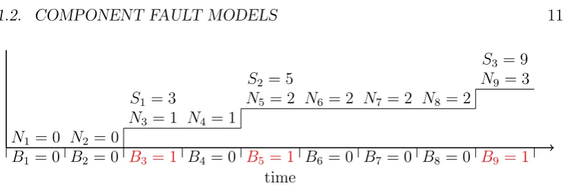
In the simplest of circumstances we can consider a processor as being in one of two states at any given time. Either it is ‘operating as intended’ or it is ‘not operating as intended’. In the state ‘not operating as intended’ we include the possibilities that the processor produces no output at all or produces incorrect output. To simplify the discussion we refer to these two states of operation as ‘on’ and ‘failed’ respectively. The state of a processor is then observed at regular intervals of length t. It is assumed that data computed in the previous interval is collected during each observation. If the processor if found to be in the failed state then all computations from the preceding interval are lost and we may therefore consider the process as being in the failed state throughout the entire interval. When a processor is observed in the failed state it is instantly replaced with another processor which is statistically identicals with respect to operating characteristics. A reasonable first failure model is to simply keep track of the proportion of times the processor was found to be in the failed state versus the total number of observations. After a sufficiently large number of observations the proportion of observations in the failed state can be used as an approximation of the probability of subsequent observations being in the failed state. This experimental setup can be modelled as a sequence of Bernoulli trials.

More formally, letB1, B2, B3, . . . be a sequence of independent and identically

distributed random variables for which each Bi denotes the state of the

proces-sor throughout the ith interval. Let Bi = 0 denote the state ’on’ and Bi = 1

(21)

time

B1 = 0

N1 = 0

B2 = 0

N2 = 0

B3 = 1 N3 = 1

S1 = 3

B4 = 0

N4 = 1

B5 = 1 N5 = 2

S2 = 5

B6 = 0

N6 = 2

B7 = 0

N7 = 2

B8 = 0

N8 = 2

B9 = 1 N9 = 3

[image:21.595.116.524.68.206.2]

S3 = 9

Figure 1.3: The Bernoulli trial model of process failure. Bi is the status of the ith

interval with 1 being a failure. The Ni are the cumulative sum of the Bi. Sj denotes the first i for which Ni ≥j.

for some p ∈ (0,1) respectively, that is Bi ∼ B(1, p) (where B(m, q) denotes

the binomial distribution having probability mass function m_kqk(1−q)m−k with

k ∈ {0,1, . . . , m}). It is implicit in this model that failure rate is constant over time. Checking the processor at the end of the ith interval is then synonymous with sampling the Bernoulli random variable Bi, also known as a Bernoulli trial.

We note that E[Bi] = (1−p)·0 +p·1 = p which is the proportion of intervals

for which the processor can be expected to be in the failed state. Additionally the variance is E[B_i2]−E[Bi]2 =p−p2 =p(1−p). Given this simple model there

are many questions one might ask:

• How many replacement processes are required over n intervals?

• What is the downtime and availability over n intervals?

• What is the time to the first failure?

• What is the expected lifetime of each processor?

The number of replacement processors required over n intervals is given by the random variableNn=Pn_i₌₁Bi (which also counts the number of failures). It

follows that the number of replacements has expectation E[Nn] =npand variance

Var(Nn) = np(1−p). The proportion of failures in n checks is given by Nn/n.

By the strong law of large numbers

Nn n

a.s.

−−−→

n→∞ E[B1] =p ,

(with Xn

a.s.

−−→x meaning Pr(Xn →x) = 1). Additionally

E

Nn n

= E[B1+· · ·+ E[Bn]]

n = np

(22)

The total downtime overnintervals is given bytNnwith expectation E[tNn] =tnp

and variance Var(tNn) = t2np(1−p). The availability is given byt(n−Nn) which

has expectation tn(1−p) and variance t2_np₍₁₋_p_{). The time to first failure is}

tS1 where Sj := mini{Ni ≥j} for j = 1,2,3, . . . which denotes the number of

intervals before the jth failure. Figure 1.3 depicts the Bernoulli trial model with the random variables Bi, Ni and Sj. As S1 =k iff Bi = 0 for i = 1,2, . . . , k−1

and Bk= 1 it follows that

E[S1] =

∞

X

k=1

kp(1−p)k−1 = p 1−p

∞

X

k=1

∞

X

i=k

(1−p)i = p 1−p

∞

X

k=1

(1−p)k

1−(1−p) = 1

p.

Therefore the expected time to the first failure is E[tS1] = _pt. The time between

failures is given bySj+1−Sj but since the rate of failure is constant the expected

time between failures is equal to the expected time to the first failure. It follows that the expected lifetime of each processor is tE[Sj+1−Sj] = _pt.

Whilst this is a very simple model there are a variety of cases where limited information about failure rates is available and this model has practical use. Suppose you have bought a processor and switch it on. The only information you may have available regarding how long that component will operate successfully may be the manufacturers rated lifetime. Suppose the processor is rated for M

continuous operating hours, then if we take M to be the expected lifetime then our Bernoulli model says E[tS1] = _pt =M and thus p = _Mt is the probability of

failure for each observation (witht the time between observations in hours). As a systems administrator you may be expected to ensure a processor is available for use for 4 years (35 064 hours). The number of observations over these 4 years is

35064

t . It follows that the number of replacements has expectation E[Nn] =np=

35064

t t M =

35064

M .

In Section 1.2.2 we will consider a renewal process model of faults. To motivate this we will consider the failure distribution the Bernoulli trial model where the length of the intervaltbetween observations vanishes. We are interested in a total time sfor which there are n=ds/teintervals. In the infinitesimal limit t→0 we assume the probability of failure in each interval is proportional tot. Specifically, letptbe the probability of failure within an interval of lengthtand limt→0 p_tt =r <

∞. We now claim that as we increase the frequency of observation, that ist→0, then the probability of observingkfailures in a fixed interval, that is Pr(Nn =k),

(23)

probability mass function

Pr(Nn=k) =

n k

pk_t(1−pt)n−k.

We may rewrite this as

Pr(Nn =k) = 1

k!(npt)((n−1)pt)· · ·((n−k+ 1)pt)

1− npt n

n−k

.

Now as n→ ∞ (and t=s/n→0) one has

npt = s

tpt→sr .

Similarly (n−1)pt → sr, . . . ,(n−k+ 1)pt → sr for fixed k. This leads to the

limit

1−npt n

n−k

=1− npt n

−k

1− npt n

n _t_→₀

−−→1− sr n

−k

1− sr n

n

n→∞

−−−→1×e−sr.

Putting the pieces together one obtains the limit

n k

pk_t(1−pt)n−k −−→ t→0

(sr)k k! e

−sr_,

which is the Poisson distribution. Thus Nn converges to a Poisson process which

is a special example of a renewal process which is introduced in the following section.

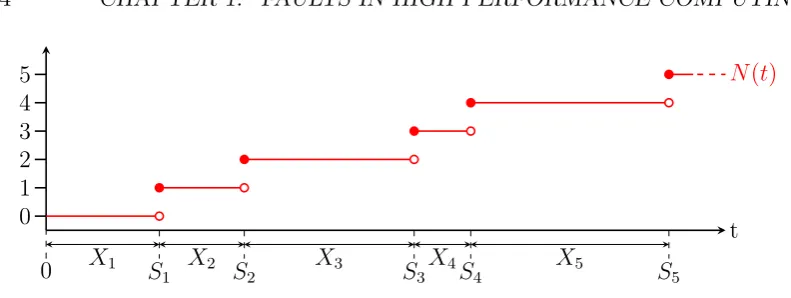
1.2.2 Renewal processes

Definition 1.1. LetX1, X2, X3, . . . be a sequence of independent and identically

distributed random variables with support [0,∞) and (strictly) positive and finite expectation (i.e. 0<E[Xi]<∞). Now for i= 1,2,3, . . . we define the sequence

of random variables Si :=

Pi

j=1Xj. Associated with theSi we have for t≥0 the

counting process

N(t) := sup{i:Si ≤t}=

∞

X

i=1

χ[0,t](Si).

which is called a renewal process.

(24)

t

0 0 1 2 3 4 5

X1 X2 X3 X4 X5

S1 S2 S3 S4 S5

[image:24.595.77.473.80.229.2]

N(t)

Figure 1.4: The renewal model of process failure. The Xi are the times between failures and the Si are the cumulative sum of the time between failures. N(t) is the renewal process and is the number of failures that have occurred up to time t.

examples. In the context of processor faults we think of the Xi as denoting the

time between the i− 1 and ith failures of a processor (which is immediately replaced with an identical processor after each such failure). Then Si is the time

at which the ith processor fails and N(t) is the number of failures that have occurred up to (and including) a given time t. An example of a renewal process is depicted in Figure 1.4.

Example 1.2. Suppose we haveXi for which the probability of failing at any

in-stant of time is 0 and the probability of failure within any interval is independent of when the interval begins. We claim that the Xi must be exponentially

dis-tributed and the corresponding renewal process N(t) is a Poisson process. More formally let X1, X2, . . . be continuous and Pr(Xi ≤t+s| Xi > t) = Pr(Xi < s)

for t, s ≥ 0. We will denote the cumulative distribution of the Xi by F(t) =

Pr(Xi ≤t). For allt, s ≥0 we have

F(s) = F(t+s)−F(t)

1−F(t) =⇒1−F(s) = 1−

F(t+s)−F(t) 1−F(t) =

1−F(t+s) 1−F(t) =⇒(1−F(s))(1−F(t)) = 1−F(t+s).

It follows that 1−F (Pn

i=1ti) =

Qn

i=1(1−F(ti)) fort1, . . . tn ≥0. Letr= 1−F(1),

then for all n= 1,2, . . . one has 1−F(n) = 1−F (Pn

i=11) = (1−F(1))

n

=rn_.

Similarly r1/n _{= (1}₋_F₍₁₎₎1/n

= (1−F (Pn

i=11/n)) 1/n

= 1−F(1/n). Thus for any convergent sequence of (positive) rationals mi

ni one has limi→∞1−F(mi/ni) =

limi→∞rmi/ni and since F is continuous it follows that 1 − F(t) = rt for all

t ∈ [0,∞). Thus F(t) = 1−etlog(r)_{, that is} _X

i is exponentially distributed with

mean _log(1_r₎ (note that r = 1−F(1) ∈ (0,1) and so log(r) < 0). Now consider the corresponding renewal process N(t) for a fixed time t. With Si =

(25)

and FSi the cumulative distribution function of Si note that via the law of total

probability

Pr(N(t) =k) = Pr(Sk ≤t < Sk+1) =

Z t

0

Pr(Xk+1 ≥t−Sk |Sk =s)dFSk(s)

=

Z t

0

Pr(Xk+1 ≥t−s)fSk(s)ds .

Now Pr(Xk+1 ≥ t−s) = e(t−s) log(r) and fSk(t) =

dF_Sk(t)

dt is given by the k-fold

convolution of the probability distribution f(t) = dF_dt(t) = −log(r)etlog(r) of each of the Xi. Assume that fSk(s) =

sk−1₍₋_log(_r₎₎k

(k−1)! e

slog(r) _{(which is clearly true for}

fS1 =fX1 =f) then

fS_k₊₁(s) =

Z s

0

fS_k(s−t)dF(t)

=

Z s

0

(s−t)k−1(−log(r))k

(k−1)! e

(s−t) log(r)

−log(r)etlog(r) dt

= (−log(r))k+1eslog(r)

Z s

0

(s−t)k−1 (k−1)! dt = (−log(r))k+1eslog(r)

−(s−t)k

k!

s

t=0

= s

k₍₋_log(_r₎₎k+1

k! e

slog(r)_.

Thus by induction fSk(s) =

sk−1(−log(r))k (k−1)! e

slog(r) _{for all} _k _{= 1}_,₂_{, . . .} _{and therefore}

Pr(N(t) =k) =

Z t

0

sk−1₍₋_log(_r₎₎k

(k−1)! e

tlog(r)

ds = t

k₍₋_log(_r₎₎k k! e

tlog(r)

.

Hence N(t) is Poisson distributed. This completes the example.

One may wish to know the average rate at which N(t) grows. As N(t) is constant except at the points S1, S2, . . . where it is discontinuous it follows that

dN(t)

dt = 0 almost everywhere. This is not a particularly useful result so we instead

study N_t(t) for larget.

Lemma 1.3 ([99, 76]). Given a renewal process N(t) with inter-arrival times

X1, X2, . . . which are independent and identically distributed (iid) one has

lim

t→∞

N(t)

t =

1 E[X1]

(26)

Proof. With Si =Pi_j₌₁Xj note that SN(t)≤t < SN(t)+1 and therefore

SN(t)

N(t) ≤

t N(t) <

SN(t)+1

N(t)

By the strong law of large numbers we have that

lim

i→∞ 1

iSi = limi→∞ 1

i i

X

j=1

Xj

a.s.

−−→E[X1].

Similarly

lim

i→∞ 1

iSi+1 = limi→∞

i+ 1

i

Si+1

i+ 1

a.s.

−−→E[X1].

Therefore given any sequence of times ti such that ti → ∞and N(ti) = ione has

ti N(ti)

< SN(ti)+1

N(ti)

= Si+1

i

a.s.

−−−→

i→∞ E[X1], and

ti N(ti)

≥ SN(ti)

N(ti)

= Si

i

a.s.

−−−→

i→∞ E[X1]. It follows that ti

N(ti)

a.s.

−−−→

i→∞ E[X1], or equivalently N(ti)/ti

a.s.

−−−→

i→∞ 1/E[X1]. (Note that the existence of the sequence ti → ∞ with N(ti) =i for alli is guaranteed

by the condition 0 <E[Xi]<∞).

Therefore for sufficiently large t one has N(t)≈ t

E[X1]. One might conjecture

that E[N(t)]/t →1/E[X1] is an immediate consequence. Whilst the conjecture

is true the proof requires some care and the result is referred to as the elementary renewal theorem.

Theorem 1.4(Elementary renewal theorem [99]). Let{N(t);t≥0}be a renewal process with mean inter-arrival time E[X1], then

lim

t→∞

E[N(t)]

t =

1 E[X1]

.

Several different proofs of this may be found in elementary texts on stochastic processes, see for example [76, 121, 113] or Cox’s monograph [35]. We include a proof here that uses the notion of stopping times similar to that in [99].

Definition 1.5. Astopping timeT for a sequence of random variablesX1, X2, . . .

is a positive integer valued random variable with E[T]< ∞ for which the event

{T ≥n} is statistically independent of Xn, Xn+1, . . . (i.e. it may only depend on

(27)

Notice that N(t) + 1 is a stopping time since the event {N(t) + 1 ≥ n} =

{Sn−1 ≤ t} depends only upon X1, . . . , Xn−1. Clearly N(t) is not a stopping

time because {N(t) ≥ n} = {Sn ≤ t} depends on Xn. The following theorem

regarding stopping times is extremely useful.

Theorem 1.6 (Wald’s equation [99]). Let X1, X2, . . . be a sequence of iid

ran-dom variables each with mean E[X1]. If T is a stopping time for X1, X2, . . ., and

E[T]<∞, and ST =PT

i=1Xi, then

E[ST] = E[X1]E[T].

Proof. We can write

ST =

∞

X

i=1

Xiχ[i,∞)(T).

As the event T ≥i is independent of Xi

E[ST] =E

" _∞ X

i=1

Xiχ[i,∞)(T)

#

= ∞

X

i=1

E[Xiχ[i,∞)(T)]

= ∞

X

i=1

E[X1]E[χ[i,∞)(T)]

= E[X1]

∞

X

i=1

Pr(T ≥i) = E[X1]E[T]

where the interchanging of the expectation of infinite sum is valid because E[T] is finite and the last equality uses the identity

E[T] = ∞

X

j=1

jPr(T =j) = ∞

X

j=1

j

X

i=1

Pr(T =j) = ∞

X

i=1

∞

X

j=i

Pr(T =j)

= ∞

X

i=1

Pr(T ≥i).

We now prove the elementary renewal theorem.

Proof of Theorem 1.4. Fix s > 0, then for i = 1,2, . . . we define the truncated random variables ˜Xi =Xi for Xi ≤s and ˜Xi = s for Xi > s. As the Xi are iid

then the ˜Xi are also iid and by considering ˜Si =

Pi

j=1X˜j we form the renewal

process ˜N(t) = sup{i : ˜Si ≤ t} for t ≥ 0. Clearly ˜Si ≤ Si implies ˜N(t) ≥ N(t)

and therefore E[ ˜N(t)]≥E[N(t)]. By Wald’s equality

(28)

and therefore since SN(t)+1 ≥t one has

E[N(t)]

t =

E[SN(t)+1]/E[X1]−1

t ≥

1 E[X1]

− 1

t . (1.1)

Similarly for the ˜Si we consider the stopping time ˜N(t) + 1 for which one has

˜

S_N˜₍_t₎ ≤ t and as ˜XN(t)+1 ≤s it follows that ˜S_N˜₍_t₎₊₁ ≤ t+s. Again by applying

Wald’s equality one obtains

E[ ˜X1](E[N(t)] + 1)≤E[ ˜X1](E[ ˜N(t)] + 1) = E[ ˜S_N˜₍_t₎₊₁]≤t+s .

Re-arranging and dividing by t we have E[N(t)]

t ≤

(t+s)/E[ ˜X1]−1

t =

1

E[ ˜X1]

+ s

tE[ ˜X1]

− 1

t . (1.2)

Now by setting s =√t and combining equations (1.1) and (1.2) one has 1

E[X1]

− 1 t ≤

E[N(t)]

t ≤

1

E[ ˜X1]

+ √ 1

tE[ ˜X1]

− 1 t

then as s → ∞ we observe that E[ ˜X1] → E[X1] and now letting t → ∞ clearly

E[N(t)]/t→1/E[X1].

A related theorem by Blackwell gives the asymptotic rate of the expected number of renewals occurring in an interval of fixed length. We give the non-arithmetic case here (a probability distribution is non-arithmetic if the distribution is concentrated on a set of equally spaced points).

Theorem 1.7 (Blackwell’s theorem [99]). Let X1, X2, . . . be positive iid random

variables which are non-arithmetic with mean E[X1]<∞ and let {N(t) :t ≥0}

be the associated renewal process. Then for any s >0

lim

t→∞(E[N(t+s)]−E[N(t)]) =

s

E[X1]

.

We note that for large t the elementary renewal theorem gives E[N(t+s)]−

E[N(t)]≈ (t+s)/E[X1]−t/E[X1] = s/E[X1]. For a rigorous proof we refer the

reader to [99].

Example 1.8. Let N(t) be the Poisson process as in Example 1.2. One has

E[N(t)] = ∞

X

k=0

k· (−tlog(r)) k

k! e

tlog(r) _{= (}_−t_log(_r₎₎_etlog(r)

∞

X

k=1

(−tlog(r))k−1 (k−1)! =−tlog(r)etlog(r)e−tlog(r)=−tlog(r),

and thus E[N_t(t)] = −log(r) = _E[_X1

1]. Notice that this is for any t ∈ [0,∞) as

(29)

The following theorem tells us about the convolution of functions with the expectation of N(t) in the limitt→ ∞ and will be used later.

Theorem 1.9 (Key renewal theorem [99, 48]). Let H(t) be directly Riemann integrable and H(t) = 0 for t < 0, X1, X2, . . . be positive iid random variables

which are non-arithmetic with mean E[X1] < ∞ and let {N(t) : t ≥ 0} be the

associated renewal process with M(t) = E[N(t)], then

Z t

0

H(t−s)dM(s)−−−→t→∞ 1

E[X1]

Z ∞

0

H(s)ds .

A full proof can be found in [48].

So far we have studied the mean of N(t)/t, of course it would also be useful to know something about the variance. The following central limit theorem holds for renewal processes.

Theorem 1.10 (Central limit theorem for renewal processes [99]). Let {N(t) :

t ≥0} be a renewal process where inter-arrival times have finite standard devia-tion σ > 0, then

lim

t→∞Pr

N(t)−t/E[X1]

σE[X1]−3/2

√ t < x

= √1

2π

Z x

−∞

e−y2/2dy .

For a proof we refer the reader to [99]. We merely comment here that the result implies that N(t) tends to a normal distribution with mean t/E[X1] and

variance σ2E[X1]−3t.

The above asymptotic results are very useful when one wishes to estimate the long term consequences of failures in a system. For example, system administra-tors can estimate the expected cost of replacing components over a long service period t by multiplying the individual cost of a component by N(t) ≈ t

E[X1]

as a result of Theorem 1.4. Similarly, a user running a job in late produc-tion (large t) for time s can estimate the expected number of failures to be E[N(t+s)]−E[N(t)] ≈ s

E[X1] as a result of Theorem 1.7. However, as the

pre-vious results are asymptotic (t → ∞) it is not clear if they may be used as estimates for relatively small t. In Example 1.8 we saw that E[N(t)] = _E[_Xt_1] for allt∈[0,∞) when the inter-arrival times are exponentially distributed. Thus one might expect that for distributions similar to that of the exponential distribution (for example, the Weibull distribution with shape parameter close to 1) then the asymptotic estimates may still be applied to small t with reasonable accuracy.

(30)

Theorem 1.11 (Renewal equation [99]). Let {N(t);t≥ 0} be a renewal process with mean inter-arrival times 0<E[X1]<∞, then

E[N(t)] = F(t) +

Z t

0

E[N(t−s)]dF(s), (1.3)

where F(t) is the cumulative distribution of the Xi.

Proof. From the law of total expectation E[N(t)] = EX1[E[N(t) | X1]]. Further,

note that forX1 > tone has E[N(t)|X1] = 0 and forX1 ≤t the renewal process

N(t)−1 from the time X1 is statistically identical to the renewal process N(t)

starting from 0, in particular E[N(t)|X1 ≤t] = 1 + E[N(t−X1)]. It follows that

E[N(t)] =

Z t

0

E[N(t)|X1 =s]dF(s) =

Z t

0

(1 + E[N(t−s)]) dF(s)

=F(t) +

Z t

0

E[N(t−s)]dF(s),

as required.

The result shows that E[N(t)] is the solution to a Volterra integral equation of the second kind. It is also related to a more convenient expression for E[N(t)]. If X1 has a probability distribution f then the renewal equation can be written

as the convolution M =F +M ∗f where M(t) := E[N(t)]. Remember that for two independent random variables X andY which have probability distributions

fX and fY respectively then the probability distribution of X +Y is given by

the convolution fX+Y(t) = (fX ∗ fY)(t) :=

R∞

∞ fX(t −s)fY(s)ds. Similarly if

FX, FY, FX+Y are the cumulative distributions of X, Y, X +Y respectively then FX+Y =FX∗fY =fX∗FY. Thus if we define Fn :=Fn−1∗f with F1 =F being

the cumulative density function (_cdf) of the Xi then FSn =FX1+X2+···+Xn =Fn.

Since N(t) = P∞

n=1χ[0,t](Si) then

M(t) = E[N(t)] = ∞

X

n=1

Pr(Sn ≤t) =

∞

X

n=1

Fn(t).

As a consistency check we note that if the probability density function (pdf) f(t) = dF_dt(t) is well-defined then

∞

X

n=1

Fn=F +

∞

X

n=2

Fn=F +

∞

X

n=1

Fn

!

∗f =F +M ∗f =M .

(31)

N(t)−1

N(t)

N(t) + 1

SN(t) t SN(t)+1

[image:31.595.119.520.93.218.2]

t−SN(t) SN(t)+1−t

Figure 1.5: Forward and backward recurrence times SN(t)+1−t and t−SN(t)

respec-tively.

Theorem 1.12 ([99]). Given F and M defined above and

h(t) = g(t) +

Z t

0

h(t−s)dF(s)

for t≥0 then

h(t) = g(t) +

Z t

0

g(t−s)dM(s).

This can be proved by taking the Laplace transform, re-arranging to get an expression forh and taking the inverse Laplace transform, see for example [99].

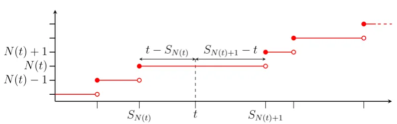
For a user logging into a compute node at a random time the most relevant question may be: what is the expected time from now until the next failure? Equivalently, given a time t at which the user logs in, he/she would like to know E[SN(t)+1−t]. This is referred to as the forward recurrence time, or sometimes

as the residual lifetime or random incidence and is depicted in Figure 1.5. The following theorem gives us an integral for calculating E[SN(t)+1−t] for a givent

as well as the asymptotic behaviour for large t.

Theorem 1.13 (Forward recurrence time [99]). Let X1, X2, . . . be positive iid

random variables with mean 0 < E[X1] < ∞ and cumulative density function

F = FX1. Let Si =

Pi

j=1Xj and N(t) be the associated renewal process with

M(t) := E[N(t)]. Then, for s, t ∈ [0,∞), the cumulative distribution of the random variable SN(t)+1−t is given by

Pr(SN(t)+1−t≤s) = F(t+s)−

Z t

0

1−F(t+s−r)dM(r). (1.4)

Further, if the Xi are non-arithmetic then

lim

t→∞Pr(SN(t)+1−t≤s) = 1 E[X1]

Z s

0

(32)

Proof. One has

Pr(SN(t)+1−t≤s) = 1−Pr(SN(t)+1−t > s)

= 1−

Z ∞

0

Pr(SN(t)+1−t > s|X1 =r)dF(r).

Ifr > t+sthenX1 > tand soN(t) = 0. ThereforeSN(t)+1 =S1 =X1 =r > t+s

and so Pr(SN(t)+1−t > s) = 1. Similarly if t < r ≤ t+s then again N(t) = 0

and therefore SN(t)+1−t =X1 −t≤s and so Pr(SN(t)+1−t > s) = 0. Lastly if

r ≤t then the process is restarted from t = r and we have Pr(SN(t)+1 −t > s |

X1 =r) = Pr(SN(t−r)+1−(t−r)> s) (i.e. shifting so that X1 is the origin gives

an equivalent renewal process). Putting the pieces together one obtains

Pr(SN(t)+1−t≤s) = 1−

Z t

0

Pr(SN(t−r)+1−(t−r)> s)dF(r)−

Z ∞

t+s

1dF(r)

=F(t+s)−

Z t

0

1−Pr(SN(t−r)+1−(t−r)≤s)dF(r)

=F(t+s)−F(t) +

Z t

0

Pr(SN(t−r)+1−(t−r)≤s)dF(r).

We can apply Theorem 1.12 to this last line to obtain

Pr(SN(t)+1−t ≤s) =F(t+s)−F(t) +

Z t

0

F(t+s−r)−F(t−r)dM(r). (1.6)

Now notice that R₀tF(t−r)dM(r) =R₀tM(t−r)dF(r) =M(t)−F(t) by The-orem 1.11. Substituting this into (1.6) leads to (1.4). To obtain (1.5) we apply Theorem 1.9 to (1.4) to obtain

F(t+s)−

Z t

0

1−F(t+s−r)dM(r)−−−→ t→∞ 1−

1 E[X1]

Z ∞

0

1−F(r+s)dr

=1− 1

E[X1]

Z ∞

s

1−F(r)dr

=1−

1− 1

E[X1]

Z s

0

1−F(r)dr

= 1

E[X1]

Z s

0

1−F(r)dr ,

as required.

It follows that the pdfof the asymptotic forward recurrence time is given by

1−F(s)

E[X1] and hence the expectation is

lim

t→∞E[SN(t)+1−t] = 1 E[X1]

Z ∞

0

(33)

If the Xi are exponentially distributed with mean µthen one obtains

lim

t→∞E[SN(t)+1−t] =µ −1

Z ∞

0

s 1−(1−e−s/µ) ds

=−se−s/µ∞

s=0+

Z ∞

0

e−s/µds=µ .

This is consistent with the memory-less property previously described. If the Xi

are Weibull distributed with scale λ and shapeκ then

lim

t→∞E[SN(t)+1−t] = 1

λΓ(1 + _κ1)

Z ∞

0

s 1−(1−e−(s/µ)κ)

ds ,

and making the substitution s7→λz1/κ _{results in}

lim

t→∞E[SN(t)+1−t] = 1

λΓ(1 + _κ1)

Z ∞

0

λz1/κe−zλ κz

1/κ−1_{dz ,}₌ λΓ( 2

κ) κΓ(1 + 1_κ).

If the user is able to access system logs and determine the time of last failure, that isSN(t), and knows something about the distribution of time between failures

(i.e. the Xi and hence XN(t)+1) then one could attempt to compute the forward

recurrence time via

E[SN(t)+1−t] = E[SN(t)+XN(t)+1−t] = E[XN(t)+1]−E[t−SN(t)].

The trick here however is that typically E[XN(t)+1] 6= E[X1]. This is known as

the inspection paradox. For example, it can be shown (similar to the proof of Theorem 1.13) that

lim

t→∞Pr(t−SN(t) ≤s) = 1 E[X1]

Z s

0

1−F(r)dr ,

and as a consequence

E[XN(t)+1] = E[t−SN(t)] + E[SN(t)+1−t] =

2 E[X1]

Z ∞

0

s(1−F(r))ds .

For exponentially distributed Xi this evaluates to 2E[X1] and thus E[XN(t)+1] is

(34)

t

0

−2

−1 0 1 2 3

S1 S2 S3 S4 S5

R1

−R2

R3

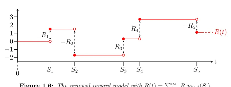
[image:34.595.75.477.88.239.2]

R4 −R5 _R₍_t₎

Figure 1.6: The renewal reward model with R(t) =P∞

i=1Riχ[0,t](Si).

A useful extension of the renewal process is the renewal reward process. The renewal processN(t) is obtained by incrementing by 1 whenever a renewal occurs, i.e. at each Si. Suppose instead we have a process R(t) which changes according

to a random variable Ri at each Si. More formally we let Ri be iid random

variables and define

R(t) :=

N(t)

X

i=1

Ri =

∞

X

i=1

Riχ[0,t](Si) (1.7)

with R(t) := 0 for N(t) = 0. An example ofR(t) is depicted in Figure 1.6. Note that theRineed not be independent ofXi, in fact many interesting examples arise

when Ri is a function of Xi. In the context of faults a renewal reward process

may be serve as a model for silent errors. Whilst the Xi determine the time

between errors the magnitude of the error can be modelled by the Ri. R(t) then

gives the sum of the errors which have occurred up to some timetthus measuring the cumulative effect. Many of the results for ordinary renewal processes can be extended to renewal-reward processes. We state a few here without proof.

Theorem 1.14 (Elementary renewal reward theorem [76, 99]). Let X1, X2, . . .

be a sequence of positive _iid random variables with finite expectation and N(t) be the associated renewal process. Further, let R1, R2, . . . be a second sequence

of _iid random variables with which we define the renewal reward-process R(t) =

PN(t)

i=1 Ri. Then with probability 1

lim

t→∞

E[R(t)]

t =

E[R1]

E[X1]

.

Similarly we have a result analogous to Blackwell’s theorem.

Theorem 1.15 ([95]). LetX1, X2, . . . be positive iid random variables which are

(35)

Further letR1, R2, . . . be iid random variables associated with the renewal-reward

process R(t) = PN(t)

i=1 Ri. Then for any0< s <∞

lim

t→∞(E[R(t+s)]−E[R(t)]) =

sE[R1]

E[X1]

.

There is also a central limit theorem for renewal-reward processes.

Theorem 1.16([126]). LetX1, X2, . . . be a sequence of positiveiid random

vari-ables with finite expectation and N(t) be the associated renewal process. Further, let R1, R2, . . . be a second sequence of non-negative iid random variables

asso-ciated with the renewal reward-process R(t) = PN(t)

i=1 Ri. If E[X 2

1],E[R21] < ∞

then

lim

t→∞Pr

R(t)−tE[R1]/E[X1]

E[(R1−X1E[R1]/E[X1])2]

p

t/E[X1]

≤x

!

= √1

2π

Z x

−∞

e−12y 2

dy .

There are many other extensions of renewal processes worth mentioning. The first is the delayed or modified renewal process where the first arrival time has different distribution then the rest. That isX2, X3, . . . areiidwith finite

expecta-tion butX1 may have different distribution (but finite expectation). An example

of this is where one starts observing a process with_iidinter-arrival times at some random time. The first observed arrival is given by the forward recurrence time whilst subsequent arrivals are identically distributed. Most of the results for ordi-nary renewal processes are easily adapted to delayed renewal processes as the first arrival does not affect the asymptotic behaviour. Alternating renewal processes occur when one has two _iid sequences X1, X2, . . . and Y1, Y2, . . . such that the

inter-arrival time Xi is followed by Yi which is then followed by Xi+1 and so on.

An example of this would be where theXi are times between component failures

and theYi are the repair times. IfN(t) is incremented at the end of each Xi+Yi

cycle then the theory for ordinary renewal processes is again easily adapted. An example relating to faults which combine both alternating and renewal reward processes is in the estimation of cumulative downtime of a system. Given _iid uptimes Xi and iid downtimes Yi then we can consider the rewards Ri =Yi

oc-curring at the end of each Xi+Yi cycle. R(t)/t then measures the proportion of

time the system was down up to timet and by applying the previous results it is straightforward to show that E[R_t(t)] −−−→

t→∞

E[Yi]

(36)

1.3 Models of many processor systems

We apply the models used for a single processor to the modelling of many pro-cessors, e.g. as in a HPC system.

1.3.1 Bernoulli processes

Consider again the simple models of Section 1.2.1 where the event of having a single processor either available or failed within a fixed interval of time is modelled as a Bernoulli trial Bi ∼ B(1, p). Now suppose we request m such identical

processors to run independently in parallel for the same fixed interval of time. Let B1,i, B2,i, . . . , Bm,i be the random variables for the state of each of the m

processors in the ith interval. We define Di := Pm_k₌₁Bk,i which is equal to the

number of processors which fail in theith interval. ClearlyDi ∼B(m, p) and the

probability of k processors fail in the ith interval is given by

Pr(Di =k) =

m k

pk(1−p)m−k.

The analysis of Di is similar to that of the Bi in Section 1.2.1. Via the

bino-mial formula it is straightforward to show that the expected number of failures throughout the ith interval is E[Di] = mp. It follows that the expected

num-ber of processors alive throughout the ith interval is m(1−p). Similarly it is straightforward to show the variance is Var(Di) = mp(1−p). As in the case of a

single process model we may ask what is the time to first failure. This is given by

S1 := min

n

j :Pj

i=1Di ≥1

o

. We note that Pr(Di = 0) = (1−p)m from which

it follows that Pr(Di ≥1) = 1−(1−p)m, therefore

E[S1] =

∞

X

k=1

k(1−p)m(k−1)(1−(1−p)m)

= 1−(1−p)

m

(1−p)m

∞

X

k=1

k

X

j=1

(1−p)mk

= 1−(1−p)

m

(1−p)m

∞

X

j=1

∞

X

k=j

(1−p)mk = ∞

X

j=1

(1−p)mj

(1−p)m =

1

1−(1−p)m .

As m increases the denominator approaches 1 from below and henceE[S1] gets

smaller. As in the single processor model, the fact that the failure rate is constant means that the mtbf is equal to the time to first failure.

(37)

are to be considered down in an interval when at least one processor fails in that interval. Thus, the expected availability of a system in these circumstances overn

intervals isn(1−p)m_{. In contrast, if the system is able to replace a failed processor}

without restarting all other processors then one may consider the availability to be the proportion of processors which are up over the n intervals. As the expected availability in one interval is m(1−p) it follows that the availability over the

n intervals is nm(1−p) which is significantly larger than the availability if all processors must be restarted whenever a failure occurs, particularly for large m. Whilst this may seem like a rather crude model it can be effective in cir-cumstances where one repeatedly runs a computation on several processes that takes roughly the same amount of time for each iteration. One can estimate the value of p by keeping track of how often processor failures occur. For example, in weather forecasting the same computation is run several times each day, every day of the year, but with different initial conditions. It is reasonable to assume that the run times do not vary significantly for each computation and therefore this model may give a reasonable estimate once the phas been estimated.

1.3.2 Superposition of renewal processes

Suppose a high performance computer consists of m (fixed integer) processors operating in parallel (independently). We assume that each of these proces-sors and their replacements have identical distributions of failure times. Let

N1(t), . . . , Nm(t) be the renewal processes associated with the life cycle of each of

the m processors. As each is processor is identical and independent each of the

Ni(t) can be assumed to be independent and identically distributed.

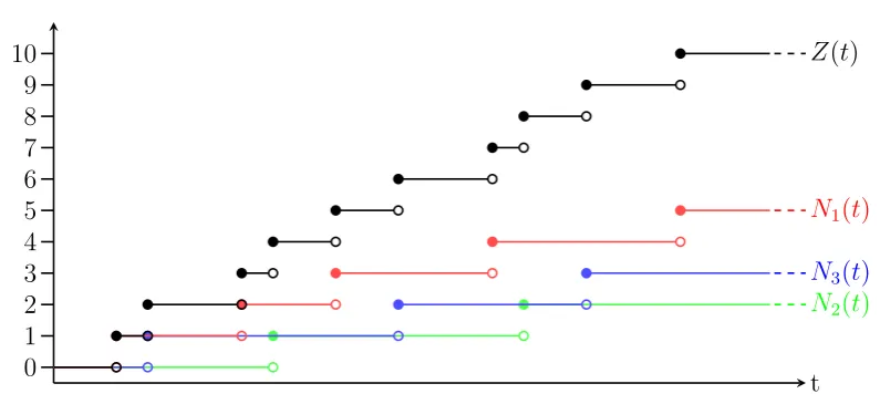
The total number of failures occurring across all m processors is given by the superposition process

Z(t) =

m

X

i=1

Ni(t).

An example is depicted in Figure 1.7. In general Z(t) is not a renewal process as it is typically not the case that inter-arrival times for Z(t) are independent and identically distributed. However, given the identical and independent nature of theNi(t) one has E[Z(t)] = mE[N1(t)] and thus results relating to the expectation

of ordinary renewal processes can be trivially applied to Z(t). For example, it follows from the elementary renewal theorem 1.4 that

lim

t→∞

E[Z(t)]

t = m

(38)

t 0

1 2 3 4 5 6 7 8 9 10

N2(t)

N3(t)

[image:38.595.77.475.93.271.2]

N1(t) Z(t)

Figure 1.7: Here we depict a stochastic process Z(t) which is a superposition of the 3

renewal processes N1(t), N2(t) and N3(t).

where E[X] is the mean inter-arrival time for all processors in the machine. Sim-ilarly Blackwell’s theorem 1.7 gives

lim

t→∞(E[Z(t+s)]−E[Z(t)]) =

sm

E[X].

Thus we immediately see that the number of processors is proportional to the asymptotic rate at which faults occur when measure over the entire timeline and within intervals of fixed length.

Example 1.17. Suppose that the time between failures for each processor are exponentially distributed and independent with mean E[X]. We know from Ex-ample 1.8 that the Ni(t) are Poisson with Pr(Ni(t) = k) = (t/E[X])

k

k! e

−t/E[X]_{. For}

m = 2 one hasZ(t) =N1(t) +N2(t) and it follows from independence that

Pr(Z(t) =k) =

k

X

i=0

Pr(N1(t) = i) Pr(N2(t) = k−i)

=

k

X

i=0

(t/E[X])i i! e

−t/E[X] (t/E[X])k

−i

(k−i)! e −t/E[X]

= (t/E[X])ke−2t/E[X] k

X

i=0

1

i!(k−i)! =

(2t/E[X])k k! e

−2t/E[X]

,

where the last equality holds since Pk i=0

k i

(39)

and assume Pr(Pm−1

i=1 Ni(t) =k) =

((m−1)t/E[X])k

k! e

−(m−1)t/E[X]_{, then}

Pr(Z(t) =k) =

k

X

i=0

Pr(Nm(t) = i) Pr(N1(t) +· · ·+Nm−1(t) =k−i)

=

k

X

i=0

(t/E[X])i

i! e

−t/E[X] ((m−1)t/E[X])k

−i

(k−i)! e

−(m−1)t/E[X]

= (t/E[X])ke−mt/E[X] k

X

i=0

(m−1)i

i!(k−i)! =

(mt/E[X])k

k! e

−mt/E[X]

,

where the last equality holds since Pk

i=0(m−1)

i k i

= mk. Thus by induction Pr(Z(t) = k) = (mt/_kE[_!X])ke−mt/E[X], that is Z(t) is Poisson distributed with mean

m times that ofN1(t). Further, this implies thatZ(t) is a renewal process in this

particular case with inter-arrival times which are exponentially distributed with mean E[X]/m. This concludes the example.

The central limit theorem forN1(t) says that Var(N1(t))→σ2tE[X]−3 ast →

∞ (whereσ2 = Var(X) is the variance of the inter-arrival time for all processors in the machine). As with the expected value, this result can be extended toZ(t) with

Pr

Z(t)−mt/E[X]

σ√mtE[X]−3/2 ≤x

t→∞

−−−→ √1

2π

Z x

−∞

e−y2/2dy .

and thus Var(Z(t))→mσ2tE[X]−3.

As with an ordinary renewal process, a random variable of interest may be the forward recurrence time. However as Z(t) is generally not a renewal process it is not immediately clear what the forward recurrence time means. However, we may take the forward recurrenceY forZ(t) to be the minimum of the forward recurrence times Yi for Ni(t), that is

Pr(Y(t)≤s) = 1− m

Y

i=1

Pr(Yi > s) = 1−(1−Pr(Yi ≤s))m.

For larget one may apply Theorem 1.13 to theYi to obtain

Pr(Yi ≤s) t→∞

−−−→1−

1− 1

E[X]

Z s

0

1−FX(r)dr

m

= 1−E[X]−m

Z ∞

s

1−FX(r)dr

m

.

(40)

for relatively small t that the behaviour of the m renewal processes ’averages out’ such that the convergence toward asymptotic behaviour is accelerated. Thus for large HPC systems the asymptotic results may be quite accurate even for relatively small t. WhilstZ(t) may not be a renewal equation in general we may consider approximating it by a renewal equation. One approach for doing this is to fit Z(t) with a renewal process such that the first few moments are the same, see for example [125]. As we already know the limiting behaviour of the mean and variance ofZ(t) a rough approximation may already be obtained using these. Consider processors where the time between failures is Weibull distributed. Schroeder and Gibson [116] and others have shown that the Weibull distribution is typically the best fit of time between failures from real fault data. The Weibull distribution with shape parameter κand scale λ has the probability distribution function

κ λ

x

λ

κ−1

e−(x/λ)κ for x≥0. (1.8)

(and 0 forx <0) which has meanλΓ(1 + 1/κ) and varianceλ2_{(Γ(1 + 2}_/κ₎₋_{Γ(1 +}

1/κ)2_{). The resulting}_Z₍_t_{) asymptotically has mean E[}_Z₍_t_)]_→_mt/₍_λ_{Γ(1 + 1}_/κ₎₎

and variance

Var(Z(t))→ mt(Γ(1 + 2/κ)−Γ(1 + 1/κ)

2₎

λΓ(1 + 1/κ)3 .

Supposing we were to approximateZ(t) with a renewal process whose inter-arrival times are also Weibull distributed with parameters κ0, λ0 we observe that κ0 =κ

and λ0 = λ/m will give the same expectation and variance in the limit t → ∞. This is consistent with the analysis of fault data by Schroeder and Gibson [116] which found that late in production the best fit of failures in a single node to be Weibull with shape 0.7 and the best fit for the entire system was also Weibull but having shape 0.78 which is close to that of a single node. Whilst the asymptotic behaviour of this approximating renewal process is the same in the first two moments, determining the how close it is to Z(t) for small t requires further investigation. This is emphasised by Schroeder and Gibson fit of faults early in production which is very different from the behaviour late in production.

1.3.3 Summary

(41)

will affect many/all processors on the same socket and/or node. However, the models considered may be analogously applied to a socket and/or node handle this type of dependence. In practice, the fault rate may also be sensitive to the workload and therefore if workload is not evenly distributed then the fault rates are likely to differ slightly. For example Schroeder and Gibson’s study [116] shows less faults occurred on weekends (when workloads are lower). Unfortunately it is not clear from their study exactly how the distribution of failure times vary with respect to workloads. It is clear that more studies need to be done into the correlation between workload and fault rate. Small variations in operating conditions could also effect the fault rate, for example the operating temperature of a node may vary slightly depending on its position in the machine room and the workload of neighbouring processors.