Selecting the number and values of the CPWI steering angles and the effect of that on imaging quality

This is a repository copy of

Selecting the number and values of the CPWI steering angles

and the effect of that on imaging quality

.

White Rose Research Online URL for this paper:

http://eprints.whiterose.ac.uk/101067/

Version: Accepted Version

Proceedings Paper:

Alomari, Z, Harput, S orcid.org/0000-0003-0491-4064, Hyder, S et al. (1 more author)

(2014) Selecting the number and values of the CPWI steering angles and the effect of that

on imaging quality. In: 2014 IEEE International Ultrasonics Symposium. IUS, 03-06 Sep

2014, Chicago, IL, USA. IEEE , pp. 1191-1194.

https://doi.org/10.1109/ULTSYM.2014.0293

© 2014 IEEE. This is an author produced version of a paper published in 2014 IEEE

International Ultrasonics Symposium Proceedings. Personal use of this material is

permitted. Permission from IEEE must be obtained for all other uses, in any current or

future media, including reprinting/republishing this material for advertising or promotional

purposes, creating new collective works, for resale or redistribution to servers or lists, or

reuse of any copyrighted component of this work in other works. Uploaded in accordance

with the publisher's self-archiving policy.

[email protected] https://eprints.whiterose.ac.uk/ Reuse

Unless indicated otherwise, fulltext items are protected by copyright with all rights reserved. The copyright exception in section 29 of the Copyright, Designs and Patents Act 1988 allows the making of a single copy solely for the purpose of non-commercial research or private study within the limits of fair dealing. The publisher or other rights-holder may allow further reproduction and re-use of this version - refer to the White Rose Research Online record for this item. Where records identify the publisher as the copyright holder, users can verify any specific terms of use on the publisher’s website.

Takedown

If you consider content in White Rose Research Online to be in breach of UK law, please notify us by

Selecting the Number and Values of the CPWI

Steering Angles and the Effect of that on Imaging

Quality

Zainab Alomari, Sevan Harput, Safeer Hyder and Steven Freear

Ultrasound Group, School of Electronic and Electrical Engineering, University of Leeds, UK.

Abstract—Compounded Plane-Wave Imaging (CPWI) has the ability to provide ultrafast imaging for many applications like colour flow imaging, microbubble imaging and elastography. The compounding operation improves the imaging quality at the expense of reducing the frame rate. Due to the importance of frame rate in ultrafast imaging, selecting the number and value of the compounded angles is a critical step to achieve the best possible imaging quality using the minimum number of angles whilst preserving the frame rate. This paper produces a new method for selecting the angular range and the number of angles in CPWI depending on the characteristics of the transducer and medium using Field II program. Experiments were performed on a wire phantom to show the efficiency of the produced method. The results show a comparative imaging quality of CPWI at the selected parameters when compared with linear imaging.

I. INTRODUCTION

In CPWI, the ultrahigh frame rates required in many ap-plications are achieved by compounding multiple unfocused images taken for the same view; each is tilted with a different steering angle [1]–[3].

The characteristics of CPWI are widely studied in the litera-ture [4]–[6]. In addition to providing ultrafast imaging, CPWI reduces the speckle level and results in higher contrast. Con-trast improvement is important in tumour and lesion detection as better borders delineation is achieved. As compared to linear imaging, CPWI can be used to achieve comparative spatial resolution and artefacts level, without restricting the imaging width by any imaging parameter, unlike linear imaging, where the width of the produced image is specified by the aperture size. However, CPWI has the disadvantages of blurring that occurs when motion exists, and having a spatial resolution that doesn’t improve with increasing the number of compounded angles [7], [8].

The lack of focusing in CPWI provides frame rates of thousands of Hertz [1] on the cost of degraded imaging quality. Compounding more angles improves this quality but lowers the frame rate, which will be divided by the number of compounded signals. A trade-off between the number of compounded angles and the frame rate should be considered in order to preserve the imaging quality and enable for ultrafast imaging in the same time. In 2004, Wilhjelm et al. produced an experimental study to calculate the angular range in CPWI [9]. They concluded through their results that the angular range of

±14◦ _{is the suitable range for steering, without considering} the transducer characteristics or the medium. Montaldo et

al. in 2009 introduced a method to calculate the number of compounded angles so that the same imaging quality as in multi-focused imaging is achieved [7]. The results gave the expected quality but the required number of angles was not suitable for ultrafast imaging.

In this paper, a method for selecting the values of the compounded angles depending on the system and medium characteristics is produced, to help achieve the required imag-ing quality usimag-ing the minimum number of angles to preserve frame rates.

II. METHODOLOGY

In CPWI, all the elements in the aperture are used to trans-mit the ultrasound beam and receive the reflected echo signal. The operation of converting the received echo signal into an image is called the beamforming. During this operation, the value assigned for each field point is calculated from the following equation [7]:

p(x, z) =

N X

j=1

Tj(t−τj(x, z)) (1)

wherexandz are the lateral and axial distances of the field point, respectively.N is the number of receiving elements and Tj(t)is the signal received by thejthelement.τj(x, z)is the time required for the signal to reach the field point and reflect back to thejth_{element, and it is calculated as follows [10]:}

τj(x, z) = zcosθ+xsinθ+

Wt

2 sin(|θ|)

c +

p

z2_{+ (xj−x)}2

c

(2) wherexj is the distance between the jth element and the centre of the transducer,Wtis the total width of the transducer, θ is the steering angle andc is the sound speed.

can be noticed from this figure that the maximum intensity at each depth is decreasing with the steering angle, and after a specific angle, the intensity starts to change randomly due to the occurrence of side lobes [13].

Fig. 1. The maximum intensity received by the field points at the centre of the transducer at a range of steering angles.

In order to find the angular range, the transducer sensitivity and medium attenuation are considered. This is done by calculating the intensity at the angular range according to the following equation:

IAR=Str+At (3)

where Str is the transducer sensitivity and At is the total amount of attenuation at the required imaging depth. De-pending on the curves of figure 1, the angle at which the maximum received intensity equals to the IAR is considered as the angular range. Angles outside this range will produce intensities that are not recognizable by the receiver. For transducers with low IAR, where all the steering angles will produce recognizable amounts of intensity, the angle at which the effect of the side lobes begins is considered as the angular range.

For wide transducers, wider beams are produced and this increases the angular range, while deeper imaging requires the use of smaller angular ranges. The angular range is plotted in figure 2 with the imaging depth for different transducer widths. This angular range was taken at the angle where the effect of the side lobes begins.

III. EXPERIMENTALSETUP

A 128-element L3-8/40EP medical probe with 0.3048 mm centre-to-centre distance was used during the experiments, driven by the Ultrasonic Array Research Platform (UARP) developed by the ultrasound group [14]–[16]. The UARP provides the control for 96 channels. Thus only 96 transducer elements were used during the experiments . The used ex-citation signal was a Gaussian pulse with a bandwidth of 5 MHz and a 5.505 MHz central frequency. A wire phantom

Fig. 2. The angular range versus imaging depth for different numbers of transducer elements.

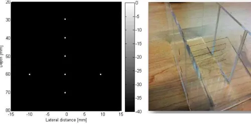
Fig. 3. (Left) The scattering points model used during lab experi-ments. (Right) The wire phantom.

with nylon wire of 0.12 mm radius was used to simulate the scattering points model, as shown in figure 3. The imaging was done in deionized and degased water.

IV. RESULTS ANDDISCUSSION

The first step in CPWI is to specify the angular range within which the steering is done, depending on the imaging system and medium specifications. The transducer used has a sensitivity of -56 dB. The imaging depth is 80 mm and the water attenuation coefficient is 0.0022 dB/MHz.mm. So that, the total amount of calculated attenuation of the medium is 0.97 dB. According to equation 3, IAR is -55.03 dB. It can be seen from figure 1 that all the angles are producing intensities of higher than IAR, and it means that they are recognizable levels of intensity. Thus, the angle at which the effect of side lobes begins will be considered as the angular range. According to figure 1, for the 80 mm depth, this range is±10◦_.

done for the same phantom with different aperture widths for comparison. The B-mode images of CPWI and linear imaging are shown in figures 4 and 5, respectively. In linear imaging, both the artefacts removal and lateral resolution were improved with increasing the aperture width, while the width of the produced image together with the depth of field were decreased with increasing the aperture width.

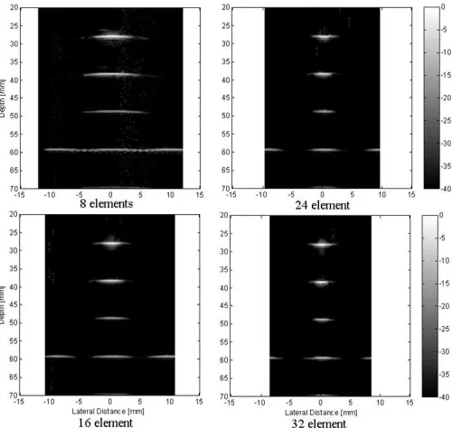
Fig. 4. CPWI imaging of the wire phantom when compounding different numbers of angles.

Fig. 5. Linear imaging of the wire phantom at different aperture widths.

In CPWI, the level of artefacts is decreased with increasing the number of compounded angles. This is because of the averaging operation that cancels the artefacts of the individual steered signals during the beamforming operation. Figure 6 shows the decrease in the artefacts level with the number of compounded angles at the sides of the 40 mm depth scattering point. It can be noticed from figures 4 and 6 that there is no decrease in the artefacts level after compounding 11 angles. This can be explained by the fact that increasing the number of compounded angles within a constant angular range results in decreasing the step between the angles and this prevents cancelling the artefacts while averaging as they intersect with each other.

Fig. 6. The artefacts level at the sides of the 40 mm depth scattering point measured when compounding different numbers of angles.

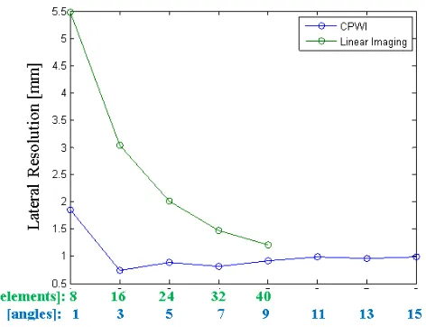
The lateral resolution at the 40 mm depth scattering point was measured for linear imaging and CPWI at the -10 dB width. The results are shown in figure 8. In linear imaging, this resolution is improved with increasing the aperture width, on the cost of lower imaging width and field of depth. This is why the aperture width was not increased to more than 40 element in the experiment. In CPWI, the lateral resolution is improved with 1.1 mm when the number of angles increased from 1 to 3. Afterwards, the resolution is decreased a little with each increase in the number of compounded angles. This is because of the averaging operation that happens between the compounded signals and results in a lateral resolution equalling to the intersected area of the individual resolutions. When the step between the compounded angles is small, then the final lateral resolution becomes wider. This is explained in figure 9, where θ₁ in (a) that represents the step between the compounded angles is smaller thanθ₂in (b). The resulted lateral resolution is indicated by the blue area.

V. CONCLUSIONS

Fig. 7. A comparison of the lateral resolution at the 40 mm depth scattering point between linear imaging and CPWI.

Fig. 8. A comparison of the lateral resolution at the 40 mm depth scattering point between linear imaging and CPWI.

and attenuation. The use of a wide angular range increases the step between the compounded angles and this increases the efficiency of compounding and results in lower level of artefacts and better lateral resolution.

REFERENCES

[1] J. Bercoff, “Ultrafast ultrasound imaging,”Ultrasound Imaging-Medical Applications, pp. 3–24, 2011.

[2] T. L. Szabo, Diagnostic ultrasound imaging: inside out. Academic Press, 2004.

[3] M. Tanter and M. Fink, “Ultrafast imaging in biomedical ultrasound,” Ultrasonics, Ferroelectrics and Frequency Control, IEEE Transactions on, vol. 61, no. 1, pp. 102–119, 2014.

[4] S. P. Weinstein, E. F. Conant, and C. Sehgal, “Technical advances in breast ultrasound imaging,” inSeminars in Ultrasound, CT and MRI, vol. 27, no. 4. Elsevier, 2006, pp. 273–283.

Fig. 9. The intersection between the individual lateral resolution of three compounded signals. Angles are: (a) −θ1,0,+θ1 (b)

−θ2,0,+θ2, where:θ2> θ1.

[5] S. Huber, M. Wagner, M. Medl, and H. Czembirek, “Real-time spatial compound imaging in breast ultrasound,” Ultrasound in medicine & biology, vol. 28, no. 2, pp. 155–163, 2002.

[6] J. Opretzka, M. Vogt, and H. Ermert, “A high-frequency ultrasound imaging system combining limited-angle spatial compounding and model-based synthetic aperture focusing,” Ultrasonics, Ferroelectrics and Frequency Control, IEEE Transactions on, vol. 58, no. 7, pp. 1355– 1365, 2011.

[7] G. Montaldo, M. Tanter, J. Bercoff, N. Benech, and M. Fink, “Coherent plane-wave compounding for very high frame rate ultrasonography and transient elastography,”Ultrasonics, Ferroelectrics and Frequency Control, IEEE Transactions on, vol. 56, no. 3, pp. 489–506, 2009. [8] P. Mohana Shankar and V. Newhouse, “Speckle reduction with improved

resolution in ultrasound images,” IEEE transactions on sonics and ultrasonics, vol. 32, no. 4, pp. 537–543, 1985.

[9] J. E. Wilhjelm, M. Jensen, S. Jespersen, B. Sahl, and E. Falk, “Visual and quantitative evaluation of selected image combination schemes in ultrasound spatial compound scanning,” Medical Imaging, IEEE Transactions on, vol. 23, no. 2, pp. 181–190, 2004.

[10] S. Korukonda, “Application of synthetic aperture imaging to non-invasive vascular elastography,” 2012.

[11] J. A. Jensen, “Users guide for the field ii program,”Technical University of Denmark, vol. 2800, 2001.

[12] ——, “Linear description of ultrasound imaging systems,” Notes for the International Summer School on Advanced Ultrasound Imaging, Technical University of Denmark July, vol. 5, 1999.

[13] H. Edwards, “Ultrasound physics and technology: How, why and when,” Ultrasound, vol. 18, no. 2, pp. 100–100, 2010.

[14] P. R. Smith, D. M. Cowell, B. Raiton, C. V. Ky, and S. Freear, “Ultrasound array transmitter architecture with high timing resolution using embedded phase-locked loops,” Ultrasonics, Ferroelectrics and Frequency Control, IEEE Transactions on, vol. 59, no. 1, pp. 40–49, 2012.

[15] S. Harput, M. Arif, J. Mclaughlan, D. M. Cowell, and S. Freear, “The effect of amplitude modulation on subharmonic imaging with chirp excitation,” Ultrasonics, Ferroelectrics and Frequency Control, IEEE Transactions on, vol. 60, no. 12, pp. 2532–2544, 2013.