A parametric finite element solution of the generalised Bloch-Torrey equation for arbitrary domains

This is a repository copy of A parametric finite element solution of the generalised

Bloch-Torrey equation for arbitrary domains.

White Rose Research Online URL for this paper:

http://eprints.whiterose.ac.uk/90964/

Version: Accepted Version

Article:

Beltrachini, L., Taylor, Z.A. and Frangi, A.F. (2015) A parametric finite element solution of

the generalised Bloch-Torrey equation for arbitrary domains. Journal of Magnetic

Resonance , 259. 126 -134. ISSN 1090-7807

https://doi.org/10.1016/j.jmr.2015.08.008

Article available under the terms of the CC-BY-NC-ND licence

(https://creativecommons.org/licenses/by-nc-nd/4.0/)

eprints@whiterose.ac.uk https://eprints.whiterose.ac.uk/

Reuse

Unless indicated otherwise, fulltext items are protected by copyright with all rights reserved. The copyright exception in section 29 of the Copyright, Designs and Patents Act 1988 allows the making of a single copy solely for the purpose of non-commercial research or private study within the limits of fair dealing. The publisher or other rights-holder may allow further reproduction and re-use of this version - refer to the White Rose Research Online record for this item. Where records identify the publisher as the copyright holder, users can verify any specific terms of use on the publisher’s website.

Takedown

If you consider content in White Rose Research Online to be in breach of UK law, please notify us by

A parametric finite element solution of the

generalised Bloch-Torrey equation for

arbitrary domains

Leandro Beltrachini

1,2

*, Zeike A. Taylor

1,3

, Alejandro F. Frangi

1,2

1

_{Centre for Computational Imaging and Simulation Technologies in}

Biomedicine (CISTIB), The University of Sheffield, Pam Liversidge

Building, Mappin St, S1 3JD, Sheffield, UK

2

_{Department of Electronic and Electrical Engineering, The University of}

Sheffield, Sheffield, UK.

3

_{Department of Mechanical Engineering, The University of Sheffield,}

Sheffield, UK.

A parametric finite element solution of the generalised

Bloch-Torrey equation for arbitrary domains

Abstract: Nuclear magnetic resonance (NMR) has proven of enormous value in the investigation

of porous media. Its use allows to study pore size distributions, tortuosity, and permeability as a

function of the relaxation time, diffusivity, and flow. This information plays an important role in

plenty of applications, ranging from oil industry to medical diagnosis. A complete NMR analysis

involves the solution of the Bloch-Torrey (BT) equation. However, solving this equation analytically

becomes intractable for all but the simplest geometries.

We present an efficient numerical framework for solving the complete BT equation in arbitrarily

complex domains. In addition to the standard BT equation, the generalised BT formulation takes

into account the flow and relaxation terms, allowing a better representation of the phenomena

under scope. The presented framework is flexible enough to deal parametrically with any order

of convergence in the spatial domain. The major advantage of such approach is to allow both

faster computations and sensitivity analyses over realistic geometries. Moreover, we developed a

second-order implicit scheme for the temporal discretisation with similar computational demands

as the existing explicit methods. This represents a huge step forward for obtaining reliable results

with few iterations. Comparisons with analytical solutions and real data show the flexibility and

accuracy of the proposed methodology.

1

Introduction

Nuclear magnetic resonance (NMR) is a powerful and non-invasive technique that allows to study

the translational motion of molecules in solution, either by diffusion or fluid flow, by using

mag-netic field gradient methods. The study of this motion reflects properties of the media and its

surrounding environment, making NMR an extremely valuable methodology for probing the

com-plex microstructure of natural and artificial materials [1]. A complete analysis of this phenomena

involves the solution of the generalised Bloch-Torrey (BT) equation [2, 3]. This equation describes

the evolution of the transverse magnetisation due to diffusion and flow in the media, spin-spin

re-laxation, and the gradient field encoding scheme. The problem of solving this equation in arbitrary

domains is of primary interest when relating variations in the acquired signals to the underlying

structures.

There has been many attempts to solve the BT equation, which can be grouped into analytical

and numerical approaches. The first group comprises solutions given by mathematical formulae

relating the output signal with parameters of interest. These solutions are obtained by proper

manipulation of the mathematical expressions describing the physical phenomena. Then,

differ-ent forms of the solution can be found depending on the mathematical framework used and the

approximations made [1, 4, 5, 6, 7]. These solutions have been shown to be very important to

study the physical basis of experimental results (e.g. [5]), as well as to perform other mathematical

analysis due to their parametric nature [1]. However, since the difficulty of such manipulation

increases with the complexity of the domain, there exist solutions only for simple geometries, as

multi-layered slabs (1D), cylinders (2D), and spheres (3D). This limits the application of these

solu-tions to arbitrary domains, restricting their usefulness to idealised models. These disadvantages are

addressed by numerical methods. This group is composed by the entire family of approximations

of the true signals obtained by the application of a numerical algorithm. Such algorithms have

the advantage of being unrestricted to simple geometries. However, they have many disadvantages

when compared to the analytical solutions, such as their non-parametric nature and the intrinsic

approximations and errors associated with them. Although the latter can be reduced in principle,

it comes at the expense of computational effort, which can be prohibitive.

There exist many numerical methods that have been used to solve the BT equation explicitly,

the finite difference method [8, 9, 10], the finite volume method [11], and the finite element (FE)

method [12, 13]. The latter is generally preferred owing to its flexibility for spatially discretising the

domain. However, many proposed solutions based on the FE method rely on strong assumptions

(e.g. narrow pulse limit approximation) that limit their general applicability. Recently, a flexible

FE formulation of the standard BT equation (i.e. without flow and transverse relaxation terms) has

been proposed [14]. There, the authors present a FE approach using first-order basis functions in

space and an explicit second-order approximation in time, which does not make such constraining

approximations. To the best of our knowledge, this latter paper by Nguyen et al. [14] is the first

to do so. Even though their approach allows to consider arbitrary geometries inside the volume

of interest, it still has limitations in the way the meshes have to be generated, imposing a hard

constraint as the symmetry of the nodal positions on the outermost faces. This adds an extra

difficulty for building and testing ad hoc models.

In this paper, we present a numerical FE framework for the solution of the complete BT equation

in arbitrarily complex domains. We extend the formulation given in [14] by considering the flow

and relaxation terms, allowing a better representation of the phenomena under scope. We obtain

parametric expressions of the corresponding matrices considering basis functions of arbitrary order.

This means that we derive closed-form formulas for all the matrices involved in the numerical

algorithm, relating explicitly the output (i.e. the resulting NMR signal) as a function of input

parameters defining the particular scenario to be tested (as diffusivities and permeabilities). These

expressions are specially useful when performing sensitivity analyses of the acquisitions to a specific

parameter, as well as to speed-up the computations [24]. Also, we broaden the formulation to deal

with both linear and parabolic spatial profiles of the magnetic field [1]. Finally, we present a second

order implicit method for the temporal discretisation. Unlike explicit schemes, implicit methods are

unconditionally stable no matter the time-step selected [26]. This is crucial for achieving reliable

solutions with a minimum number of iterations. We introduce an implicit scheme to solve the BT

equation with similar computational load as the explicit method used in [14], which makes it highly

competitive in the field. The presented framework is built on the basis of arbitrary discretisations

without imposing special constraints to the geometrical meshes to be used.

The paper is organised as follows. In Section 2 we present the mathematical basis of the problem

and the corresponding FE solution. First, we review the differential formulation in Section 2.1.

In Section 2.3 we define the volume and area coordinate systems, which have a key role in the

parametric formulation detailed in Section 2.4. The temporal discretisation of the BT equation is

described in Section 2.5. In Section 3 we show the capabilities of the numerical framework and

compare them with analytical solutions and real data. Finally, in Section 4, we discuss the results,

limitations of the approach, and further work.

Notation: In the following, we denote vectors with boldface lower case letters and matrices

with boldface capital letters. We use vec(·) to refer to the operator that, given a matrix, returns

a vector with the matrix elements stacked columnwise, taking the columns in order from first to

last. We express the Kronecker matrix product by ⊗, and the nth Kronecker product of A with itself by A⊗n. Finally, we denote the n×n identity matrix as In, and them×n matrix full of ones as 1m,n.

2

Methods

The generalised BT equation represents the evolution of the magnetisation as a function of the

spatial location and time in the absence of the RF field. Basically, it relates the evolution of the

complex-valued transverse magnetisation with four mechanisms: diffusive migration of the

spin-bearing particles, magnetic field encoding, transverse spin-spin relaxation, and flow [1, 2]. The

problem statement is completed after selecting the corresponding boundary and initial conditions.

These conditions allow to represent arbitrary situations where to study the phenomena. Once the

solution is found, it is used to describe the macroscopic signal formed by the spin ensemble.

As mentioned in Section 1, solving the BT equation analytically becomes intractable for all but

the simplest geometries. In this section, we describe the numerical framework used to solve the

aforementioned equation in arbitrary geometries and conditions. The advantages of the formulation

are explained in detail.

2.1 Differential formulation

Let Ω be the domain under analysis, which can be split intoLsubdomains, such that Ω =SL_l=1Ωl. Also, let Γe_l be the external boundary of Ωl, and Γlnthe boundary between Ωland Ωn. Then, under

generally valid assumptions (such as considering normal or Fickian diffusion, intermediate layers

see [2, 6] for a detailed discussion), the evolution of the complex transverse magnetisation ml(r, t) in the rotating frame is described by [2, 15]

∂ml(r, t)

∂t =∇ · Dl(r)∇ml(r, t)

−iγB(r, t)ml(r, t)− 1

Tl

ml(r, t)−v(r, t)· ∇ml(r, t) (r∈Ωl), (1)

subject to the boundary conditions (BCs)

Dl(r)∇ml(r, t)·nl(r) =κln mn(r, t)−ml(r, t)

(r∈Γln, ∀n), (2a)

Dl(r)∇ml(r, t)·nl(r) =−κelml(r, t) (r∈Γel), (2b)

and the initial condition (IC)

ml(r,0) =ρl(r), (r∈Ωl), (3)

wheret∈[0, TE] withTE echo time, γ is the gyromagnetic ratio of protons (2.675×108rad T−1s−1 for 1_{H), D}

l(r) is the diffusion (rank-2) tensor, Tl is the spin-spin relaxation time, v(r, t) is the velocity field of the spins due to flow of the medium, nl(r) is the unitary outward pointing normal

to Ωl,κln(κel) is the permeability constant in Γln(Γel), andB(r, t) is the effective magnetic field. In the following analysis we considered Tl constant in each subdomain Ωl and the same permeability in both directions of the same membrane, i.e. κln=κnl.

Eq. (1) states that the transverse magnetisation evolves due to diffusion (first term), encoded

through the applied magnetic field (second term), bulk relaxation (third term), and flow (last term).

The BC (2a) accounts for the creation of the diffusive flux by the drop in magnetisation between

layers. Noting that Γln = Γnl, it is easily seen that it also accounts for the conservation of the

magnetisation flux between adjacent layers, i.e.

Dl(r)∇ml(r, t)·nl(r) =−Dn(r)∇mn(r, t)·nn(r) (r∈Γln).

The flux conservation at the external boundary is considered by Eq. (2b). Finally, Eq. (3) represents

the solution of (1) for the initial state (t= 0s).

Once the complex magnetisation is computed, the output signal can be found by

S =

Z

Ω

m(r, T E)ρe(r)dr, (4)

2.2 Variational formulation and spatial discretisation

The transverse magnetisation is obtained by solving (1)–(3). This problem requires a solution

twice differentiable, thus restricting the solutions space. To relax this condition, a solution in the

weighted residual sense is obtained [16]. This solution satisfies

∂ ∂t

Z

Ωl

v(r)ml(r, t)dr=

Z

Ωl

v(r)∇ · D(r)∇ml(r, t)

dr−iγ

Z

Ωl

v(r)ml(r, t)B(r, t)dr

− 1

Tl

Z

Ωl

v(r)ml(r, t)dr−

Z

Ωl

v(r)v(r, t)· ∇ml(r, t)dr,

(5)

valid for r ∈ Ωl (l = 1, . . . , L), and for all functions v(r) in a proper functional space. The Hilbert-Sovolev spaceH1(Ωl) of square-integrable functions with square-integrable derivatives [17]

is generally chosen. After using the divergence theorem in the diffusion term and the BCs, we get

∂ ∂t

Z

Ωl

v(r)ml(r, t)dr=−

Z

Ωl

∇v(r)· Dl(r)∇ml(r, t)

dr−iγ

Z

Ωl

v(r)ml(r, t)B(r, t)dr

− 1

Tl

Z

Ωl

v(r)ml(r, t)dr−

Z

Ωl

v(r)v(r, t)· ∇ml(r, t)dr (6)

−κe_l

Z

Γe l

v(r)ml(r, t)dr+

X

n

κln

Z

Γln

v(r) mn(r, t)−ml(r, t)

dr,

also known as thevariational formulation[18]. The solution under scope needs to beonlyone-time

differentiable.

In order to obtain a discretisation of (6), it is necessary to find a solution belonging to Vh, a

finite-dimensional subspace of H1(Ωl). Let

ϕl

1(r), ϕl2(r), . . . , ϕlN(r) be a basis of Vh such that for allg(t)∈ Vh,g(t) =PNi=1ϕli(r)ηi(t), withηi(t)∈C. Then, the approximation of the transverse magnetisation m∗

l(r, t)∈ Vh satisfying (6) is defined as

m∗

l(r, t) = N

X

i=1

ϕl_i(r)η_il(t). (7)

In the case of choosing the test functions as the basis functions, i.e. v(r) =ϕl

j(r) (j= 1, . . . , N), it is possible to obtain (after some algebra)

Ml

∂η_l

∂t =−

Sl+ iQl(t) + 1

Tl

Ml+Jl(t) +Fl

η_l−X

n

where

{Ml}ij ,Mij =

Z

Ωl

ϕl_i(r)ϕl_j(r)dr, (9a)

{Sl}ij ,Sij =

Z

Ωl

∇ϕl_j(r)TDl(r)∇ϕli(r)dr, (9b)

{Q_l(t)}_ij ,Qij(t) =γ

Z

Ωl

ϕl_i(r)ϕl_j(r)B(r, t)dr, (9c)

{Jl(t)}ij ,Jij(t) =

Z

Ωl

ϕl_j(r) v(r, t)· ∇ϕl_i(r)dr, (9d)

{Fl}ij ,Fij =κel

Z

Γe l

ϕlj(r)ϕli(r)dr, (9e)

{Hln}ij ,Hij =κln

Z

Γln

ϕl_j(r)ϕl_i(r)−ϕn_i(r)dr. (9f)

Therefore, the problem turned out to find η(TE) satisfying (8). Then, it is necessary to define the basis functions needed to compute (9). For this reason, the volume and area coordinate systems

are utilised.

2.3 Volume and area coordinates

To proceed with the spatial discretisation, the volume coordinate system is introduced. As shown in

the following sections, this coordinate system allowed to compute analytically (9a)- (9d) considering

polynomial basis functions over a tetrahedral discretisation of the domain.

Let V be the volume of the tetrahedronω with nodes p_i (i= 1, . . . ,4). For any point r inside the tetrahedron, the coordinates ξi = Vi/V (i = 1, . . . ,4) are defined, where Vi is the volume of the tetrahedron with nodesr and p_j, with j6=i(j = 1, . . . ,4). Then, the volume coordinates are obtained by the transformation

ξi=

ai+bix+ciy+diz

6V , i= 1,2,3,4, (10)

whereai,bi,ci, anddi are real coefficients depending on the nodes coordinates [19]. In matrix form

ξ= 1

6V a+Λ

T_{r, (11)}

wherea,b,c, anddare the 4×1 vectors with elementsai,bi,ci, anddi, respectively (i= 1,2,3,4), Λ = [b,c,d]T, and ξ = [ξ1, ξ2, ξ3, ξ4]T. It is easily seen that (11) transforms ω into a normalised tetrahedron ωn in the ξ coordinate system. Also, it is useful to note that, sincepi 6=pj for i6=j is assumed, a,b,c, and dare linearly independent, so ΛΛT is invertible, and

is uniquely defined.

The introduction of the volume coordinates has multiple purposes. First, it allows to choose

Vh and the corresponding basis functions. In this case, and for simplicity, Vh was chosen to be

the space of piecewise polynomials up to order n0. In case of considering polynomials of degree

n0=i+j+k+l in each element, the basis functions are defined by [20]

ϕijkl(ξ) =Ri(n0, ξ1)Rj(n0, ξ2)Rk(n0, ξ3)Rl(n0, ξ4), (13)

where

Rm(n0, ξ) = 1

m! m_Y−1

k=0

(n0ξ−k). (14)

Second, it allows to evaluate analytically integrals of the form

Z

ω

ξ₁aξ₂bξ₃cξ₄ddω= 6V a!b!c!d!

(a+b+c+d+ 3)!. (15) This will be shown to be the key to obtain parametric expressions for the FE formulation.

A similar analysis can be used to define the area coordinates for the interpolation and integration

over triangles, which is mandatory to solve (9e) and (9f). Givenrinside the triangleωof areaA, the area coordinates are defined as ξi =Ai/A (i= 1,2,3), whereAi is the area of the triangle defined by r and p_j, with j 6= i (j = 1,2,3). Then, the interpolating functions of degree n0 = i+j+k are [20]

ϕijk(ξ) =Ri(n0, ξ1)Rj(n0, ξ2)Rk(n0, ξ3). (16)

Finally, the integration formula transforms to

Z

ω

ξa₁ξ₂bξ₃cdω= 2A a!b!c!

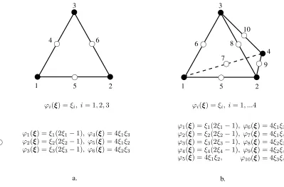
(a+b+c+ 2)!. (17) In Fig. 1 the disposition of nodes for triangles and tetrahedrons are shown, as well as their

corresponding first and second order polynomial basis functions, i.e. n0 taking values 1 and 2.

2.4 Formulation of element matrices for polynomial basis functions

It is now possible to obtain numerical representations of (9a)-(9f) using the volume and area

co-ordinate systems. To this end, the linear and quadratic basis functions were considered, achieving

first and second order FE formulations. Since these basis functions are defined for each tetrahedron

(or triangle), expressions of (9a)-(9f) valid for each element were derived, usually called

Once the basis functions are chosen, the computation of Me is straightforward. To

discre-tise (9b), it is useful to note that the gradient of any function f(r) can be expressed in the volu-metric coordinate system as∇f(r) = ₆1_VΛ∇ξf(ξ). Then, the elementary stiffness matrix is found to be

Se= 1 6Ve

Z

ωn

∇ξϕ(ξ)TΛTDΛ ∇ξϕ(ξ)dωn, (18)

where ∇ξϕ(ξ) =∇ξϕ1(ξ), . . . ,∇ξϕN(ξ)

. If the diffusion tensor is assumed constant within the

element, it is possible to extract it (as well asΛ) outside the integral. This allows to separate the

elementary matrix as the product of a coefficient (i.e. constant) matrix and a parametric matrix

dependent on the diffusion tensor elements. To this end, the vec(·) operator is utilised. Employing

the identity vec (ABC) = CT ⊗Avec(B) [21] on (18) leads to

vec (Se) = 1 6Ve

ST

Λ⊗2

T

vec(D), (19)

where

S =

Z

ωn

∇ξϕ(ξ)

⊗2

dωn, (20)

is a constant matrix once the basis functions are selected. In the particular case of choosing first

order basis functions,∇ξϕ(ξ) =I4, resulting inS =I16/6.

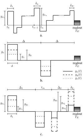
To obtain the representation of Qe(t), it is first needed to select the spatial profile of the magnetic field B(r, t). As in [1], two options were considered. The first was the commonly used linear magnetic field, in which caseB(r, t) =g(t)·r, withg(t) being the effective applied gradient field, which can vary over time (Fig. 2). In this case, inserting (12) into (9c), we obtainedQe

ij(t) = g(t)·Q(1)_ij , Q(2)_ij , Q(3)_ij , whereg(t) =gx(t), gy(t), gz(t)

T

. In matrix notation,

Qe(t) =gx(t)Q(1)e +gy(t)Q(2)e +gz(t)Q(3)e , (21)

whereQ(ek) (k= 1,2,3) are matrices defined by

h

vecQ(1)_e ,vecQ(2)_e ,vecQ(3)_e iT = 6γVe ΛΛT

−1 Λ

6VeQlin−a vec (Me)T

, (22)

where

Q_lin =

Z

ωn

ξϕ(ξ)T⊗2dωn, (23)

and ϕ(ξ) =ϕ1(ξ), . . . , ϕN(ξ)

The second option considered was to apply the normalised isotropic parabolic magnetic field,

whereB(r) =g2 r·r, withg2 constant, which is considered as a paradigm for nonlinear fields [1]. In this case, after tedious manipulations, we obtained

vec (Qe) =γg2

216V_e3Q_quad+ vec (Me) aT⊗2−72V_e2 a⊗Q_linT vec Λ, (24)

whereΛ=ΛT ΛΛT−T ΛΛT−1Λ and

Q_quad=

Z

ωn

ϕ(ξ)ξT⊗2dωn. (25)

Computing (9d) requires adopting a model for the velocity field. Assuming v(r, t) =v(r)h(t), it is found

Je=h(t)

Z

ω

∇ϕ(r)Tv(r)ϕ(r)Tdω. (26)

In the particular case of considering constant velocity in each element,Je turns out to be

vec (Je) =h(t)JΛTv, (27)

where

J =

Z

ωn

ϕ(ξ)⊗ ∇ϕ(ξ)dωn. (28)

The computation of Fe_l was straightforward when using the area coordinate system. Finally,

to compute (9f), a discontinuous FE approach was considered. Under this method, the solution

is allowed to be discontinuous at the compartment interfaces but not inside each region [14]. The

discretisation was then obtained by doubling the nodes at the interfaces, each of them belonging to

each region. Corresponding triangles share the basis functions (but not the nodes), henceHe was

easily found integrating, as done forFe_l. The resulting elemental matrix for corresponding triangles

belonging to different sides of the same boundary (i.e. corresponding toη_ln= [ηT_l ,ηT_n]T_{) is}

He_ln=κln

  

Fe −Fe

−Fe Fe

  ,

whereFe=R_ωϕ(r)ϕ(r)T_{dω (and consequentlyF}e l =κelF

e ).

Once the basis functions were chosen, the computation of the elemental matrices was achieved

by performing algebraic manipulations, more tedious as the order of the basis functions increased.

To avoid mistakes, the Symbolic Toolbox in Matlab (MathWorks Inc., Nattick, USA) was utilised

for computing the corresponding matrices using both linear and quadratic basis function sets, as

2.5 Temporal discretisation

Once the spatial discretisation is obtained, Eq. (8) needs to be solved for all Ωl (l= 1, . . . , L). For simplicity, theLsystems of differential equations are merged into a single one. The global matrices involved in (8) are then defined as the assemble of the corresponding matrices in any region. Then,

Eq. (8) could be expressed as

M∂η(t)

∂t =− Υ(t) + iQ(t)

η(t), (29)

where Υis the real part of the right term of the assemble, comprising the matrices S,M,J, F,

and H, and the lack of subindex refers to the global matrix. Most of the matrices were block

diagonal, as seen from their definitions in (9). This was extremely useful when computing inverse

matrices utilising, for example, Schur complements.

In the sequel, two different approaches to obtain η(TE) from (29) are presented, highlighting their pros and cons. Onceη(TE) is obtained, the corresponding signal is found through (4) and (7), i.e.

S=

Z

Ωe

ρ(r)m(r, TE)dr

≈X

e

Z

ωe e

ρ(r)ϕ_e(r)dr

T

η_e(TE) =

X

e

yT_eη_e(TE) =yTη(TE),

(30)

where

y_e=

Z

ωe e

ρ(r)ϕ_e(r)dr. (31)

2.5.1 Matrix exponential

The most direct method to obtain η(TE) given η0 ≡ η(0) is considering the matrix exponential function [25]. In the following, it is assumed that the matrices Υ and Q are piecewise constant

in [0, TE]. This means that the temporal flow profile and the effective magnetic gradient profile are considered to be constant within each interval of finite durationδk=tk−tk−1 (k= 1, . . . , N). The first hypothesis is not only fulfilled when studying just the diffusivity of the material, where

the flow is generally considered to be zero [1], but also when studying constant flow, as blood in

autoregulated capillaries [22]. The second arises in most commonly used sequences [1]. Under these

assumptions the acquired signal turns out to be

S =yT N

Y

k=1

e−M−

1

(Υk+iQk)δk !

whereΥkandQ_kare the constant expressions of the corresponding matrices inδk, and the product by each new matrix is leftwise. Note that the matrix products involved are in general not

commu-tative, and therefore (32) cannot be further simplified without making additional assumptions.

Eq. (32) is a valuable result for several pulse excitation sequences and applications. Although

this formula is valid only for piecewise constant gradient profiles, it can be used as a good

approx-imation to arbitrarily complex sequences, as done in the matrix formalism approach for diffusion

studies [1]. Moreover, since it is an expression depending on physical parameters, such as

permeabil-ities and diffusivpermeabil-ities of the media, it allows to perform other analytical analysis. A straightforward

example is the computation of the sensitivity of the output to these constants considering arbitrary

domains. This was proven to be useful in many applications, such as to compute performance

bounds for solving the inverse problem [23, 24].

It is of particular interest to obtain parametric expressions of the measured signals for sPGSE

and dPGSE sequences. For simplicity, let us define the matrices E∆k =e

−M−1_Υ

k(∆k−δk)_,Eδ k =

e−M−

1

(Υk+iQk)δk

, and Emk = e

−M−1_Υ

k(tm−δ1)_{. Then, in Appendix B, it is shown that the}

measured signal is given by

Ss=yTE∆1M

−1_E∗ δ1M E

T

∆1Eδ1η0, (33)

when considering sPGSE, and

Sd=yTEδ2E∆2M

−1_E∗

δ2M EmM

−1_E∗

δ1M E∆1Eδ1η0, (34)

in case of using dPGSE. Note that Eqns. (33) and (34) depend on the calculation of less matrix

exponentials than indicated by (32), hence drastically reducing the computation cost.

The expressions (32)–(34) are examples of closed-form solutions that are useful for both

the-oretical and numerical purposes. For example, it is possible to compute derivatives of Eqs. (33)

and (34) with respect to different parameters (describing the system and MR sequence),

neces-sary for performing sensitivity analyses. However, these solutions are computationally expensive

even for small problems and efficient algorithms [25], demanding a notorious amount of memory.

2.5.2 Second order numerical scheme

As in [14], the solution vector in (29) is split into its real and imaginary parts, resulting in the

following the coupled system of equations

  

M∂ηR(t)

∂t =−Υ(t)ηR(t) +Q(t)ηI(t) M∂ηI(t)

∂t =−Υ(t)ηI(t)−Q(t)ηR(t)

, (35)

whereη(t) =η_R(t) + iη_I(t). To solve this system, the implicit trapezoidal method [26] was chosen. This is a second-order scheme characterised for being the only A-stable multistep method. Since

this is an implicit method, it will generally demand a larger computational cost. However, in the

sequel, we show that this problem can be solved.

Under this scheme, Eq. (35) takes the form

    

ηn_R+1 =ηn_R+ ∆₂t−Υen+1ηnR+1+Qen+1ηnI+1−ΥenηnR+QenηnI

η_In+1 =ηn_I + ∆₂t−Υne +1ηnI+1−Qen+1ηnR+1−Υnηe nI −QenηnR

, (36)

where ∆t is the time-step length and the tilde indicates premultiplication of the corresponding matrix by M−1. Some tedious manipulations yield

    

ηn_R+1= IN +h2R2n

−1

h(Ln+RnPn)ηnI + Pn−h2R2n

ηn_R

ηn_I+1=−hRnη_Rn+1−hLnηn_R+Pnηn_I

, (37)

whereh= ∆t/2,Ln= (M +hΥn+1)−1Qn,Rn= (M +hΥn+1)−1Qn+1, and

Pn = (M +hΥn+1)−1(M−hΥn). From (37), two inverse matrices need to be computed, in-stead of one as required by any other explicit method. However, since the absolute values of the

eigenvalues ofh2R2_n are less than unity, it is possible to write [27]

IN +h2R2n

−1 =

∞

X

k=0

(−1)k(hRn)2k≈IN−(hRn)2+ (hRn)4, (38)

which reduces the needed inversion to one.

The proposed numerical scheme presents some advantages when compared to the

Runge-Kutta-Chebyshev algorithm [14]. First, the selected method is A-stable, and therefore stable irrespectively

of the selected temporal discretisation step. Second, it only needs one matrix inversion, which in

3

Numerical results

In this section we present two examples in which the capabilities of the numerical method were

tested. The first was intended to show how the developed method performed in situations where

the analytical solution was available [6], whereas the second presented a real application based

on experimental data [5]. These examples were chosen between many others just to show the

capabilities of the FE formulation in concrete situations. It is worth to mention that the eigenvalue

condition stated in Section 2.5.2 was met in every single experiment.

3.1 Bi-layered sphere

We simulated a sPGSE sequence (δ= ∆ = 10ms) in a bi-layered spherical domain with radiir1,2= [2.5,5] µm, isotropic diffusivities D1,2 = [2,2]× 10−9 m2/s, innermost (outermost) permeability

κ12 = 10−5 (κe2= 10−9), and bulk relaxivitiesT1,2 = [0.1,0.1]s. This situation represents a typical scenario when analysing biological samples, as cells or axons [6].

To account for the errors, we computed the relative error, defined as

Error= max g

kSa(g)−Sn(g)k

kSa(g)k

, (39)

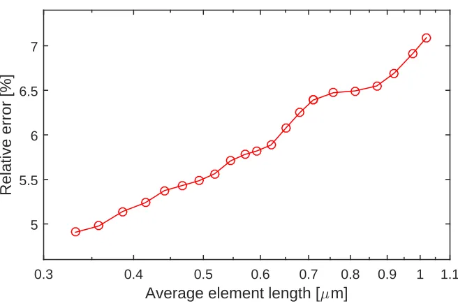
where Sa and Sn are the analytical and numerical solutions, respectively, and |g| ∈[0,1] T/m. In Fig. 3 we show the relative error for different model discretisations (obtained using the ISO2Mesh 2013

toolbox [28]) as a function of the mesh size. We considered the first order spatial discretisation

scheme (n0 = 1) and the second order temporal scheme with 100 time steps. It is seen that the numerical approach gives accurate results even using a coarse discretisation.

One of the main advantages of the presented framework is the possibility to use coarser temporal

discretisations without turning the scheme unstable. To illustrate this, we considered a spatial

discretisation consisting in 11464 elements (2198 nodes) and solved the aforementioned problem for

varying time-steps. The purpose of this experiment was to test the convergence rate of the developed

second order algorithm, and compare it with a similarly obtained first order implicit scheme. The

small number of nodes allowed us to use the graphical processing unit (GPU) to speed-up the

simulations. Although general-purpose GPUs’ memory is limited to 1-2Gb, the acceleration they

provide turns them into a preferable device where to perform demanding computational simulations.

In Fig. 4 we show the relative error as a function of the temporal discretisation for both backward

nature of both algorithms is clearly appreciated, as well as the advantage of the second order

method over the backward Euler approach.

3.2 Cylinder with dPGSE sequence

To show the versatility of the numerical framework, we simulated the last experiment reported

in [5]. It consists in the application of a dPGSE sequence (δ1 =δ2 = 4.5 ms, ∆1 = ∆2 = 40 ms,

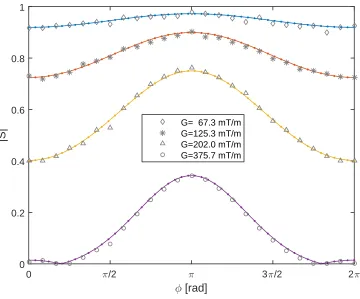
tm = 0s, gx = gy = 67.3, 125.3, 202.0, and 375.7 mT /m, gz = 0) perpendicular to impermeable cylindrical microcapillaries of inner diameter 10±1 µm, oriented in the z direction, and centred in the origin. This experiment was carried out to study the dependence of the signal decay on the

azimuthal angle between gradients. To do so, the first gradient was fixed along the x direction while the orientation of the second gradient was varied in the xy plane. We refer to [5] for more details.

We considered the first order FEM approach. We discretised cylinders of 10µm length and diameters 10.0, 10.3, 10.4, and 10.4 µm (as presented in [5]) in 750 nodes using ISO2Mesh. The reason to use a coarse spatial discretisation was to test its validity using the GPU. We refined the

temporal discretisation until no more improvement was obtained, resulting in 3000 time-steps for

this particular problem. In Fig. 5 we show both experimental and numerical results. There we

plotted the acquired signal as a function of the angle φ between gradients. There is a very close agreement between the experimental results and the numerical simulations, even using a coarse

mesh, confirming their validity for real-scenario experiments.

4

Discussion and conclusions

We presented a FE formulation for solving the complete BT equation in general domains. This

method allows to simulate MR signals in realistic scenarios, including arbitrary geometries,

physi-cal properties of the material (diffusivities, permeabilities, relaxivities, and flow), and MR settings

(sequences, field, and voxel volume). We obtained expressions for first and second order

discretisa-tions in both spatial and temporal domains. These expressions were flexible enough to work with

arbitrary discretisations, not being restricted to symmetric meshes nor to specific step lengths to

guarantee numerical stability (as in [14]). We showed its feasibility and flexibility to solve real

Unlike existing approaches, we obtained ad hocformulae for computing the matrices involved

in the numerical algorithm. This was shown to be helpful for avoiding errors due to numerical

integration, as well as to increase the speed-up. As in [6] (and differently from [14]) we considered

mixed BCs imposed on the boundaries of the simulated structures. Whether these conditions are

more suitable than the periodic BCs considered in [14] needs to be further explored. This could be

easily addressed using the developed technique on the transformed BT equation [14], and will be

the focus of future studies.

One of the major results was a second order implicit numerical algorithm for solving the

tempo-ral discretisation of the BT equation. Implicit methods have the advantage (over explicit methods)

of presenting stability properties that allow to choose coarser discretisations without

compromis-ing the validity of the result. However, implicit methods are generally discarded for solvcompromis-ing large

problems due to their computational load. In this paper, we adapted two implicit methods for

solving the temporal discretisation with similar requirements than explicit methods, hence

drasti-cally reducing the simulation time. This was highly efficient when compared to explicit methods,

which require really small step-sizes to achieve stable results [14]. Future studies will be focussed on

making these methods even more efficient by allowing an adaptive step-length selection depending

on the applied sequence.

We also presented expressions relating the measurements with parameters of interest describing

both the media under analysis and the applied sequence. This is of special interest for designing

optimal protocols to tackle specific problems, as done in brain related studies with the Cram´er-Rao

bound [29, 30, 31]. Differently from the existing analytical expressions, they allow to deviate from

standardised and simple domains and consider the real shape and physics under scope. This could

result in better ways where to apply parametric tools for MR protocol optimisation and design.

Acknowledgements

The authors thank Dr. D. Grebenkov for sharing the Matlab toolbox implementing the sPGSE

of restricted diffusion in multi-layered structures. The work has been supported by the

Euro-pean Commission FP7 project VPH-DARE@IT (FP7-ICT-2011-9-601055) and the project OCEAN

A

Results considering linear basis functions

The computation of the matrices involved in the FE discretisation can be easily computed once

the basis functions set is chosen. After transforming the corresponding integrals to the volume or

area coordinate systems, exact results were obtained using (15) and (17). In the special case of

considering linear basis functions, we get

Me = Ve

20(14,4+I4), (40a) Se= 1

36Ve

ΛTDΛ, (40b)

Q_lin= [K₁,K₂,K₃,K₄], (40c)

Q_quad=

                                                

24 6 6 6 6 4 2 2 6 2 4 2 6 2 2 4

4 2 2 4 6 2 2 2 2 2 1 2 2 1 2

4 2 2 2 2 1 4 2 6 2 2 1 2 2

4 2 2 1 2 2 1 2 2 4 2 2 6

4 6 2 2 2 2 2 1 2 2 1 2

24 6 6 2 6 4 2 2 6 2 4

4 2 2 4 6 2 1 2 2 2

4 1 2 2 2 2 4 2 6

4 2 6 2 2 1 2 2

4 6 2 1 2 2 2

24 6 2 2 6 4

4 2 2 4 6

4 2 2 6

4 2 6

4 6 24                                                  , (40d)

J = 1

24(14,1⊗I4), (40e) Fe= Ae

12 (13,3+I3), (40f)

applied when considering second order basis functions.

B

Signal models for sPGSE and dPGSE sequences

To obtain (33) and (34) we first need a useful identity. Using matrix exponential properties and

the fact that M,Υ, and Q are symmetric matrices, it is straightforward to show

e−M−

1

(Υ±iQ_{) =M}−1_e−M−1

(Υ∓iQ)∗_{M, (41)}

where ∗ _{denotes conjugate transpose. In case of performing a sPGSE experiment, the measured}

signal is given by

S =yTE∆Eδ3E∆Eδ1η0, (42)

where Eδ1 and Eδ3 account for the first and second gradient pulses, respectively, and E∆ for the

intervals without imposed magnetic field gradient. Since both effective magnetic gradient pulses

have the same duration (δ) and opposite magnitude (Fig. 2b), we can replace Q₃ inEδ3 by−Q1. Then, using (41) we get Eδ3 =M

−1_E∗

δ1M, and consequently (33). For computational purposes it is worth to note thatE∆M−1 =M−1ET∆. A similar analysis can be used to prove (34).

References

[1] D. Grebenkov, NMR survey of reflected Brownian motion, Rev. Mod. Phys., 79 (2007) 1077–

1137.

[2] J. Jeener, Macroscopic Molecular Diffusion in Liquid NMR, Revisited, Conc. Magn. Reson.,

14 (2002) 79–88.

[3] W. Price, NMR Studies of Translational Motion: Principles and Applications, Cambridge

University Press, UK, 2009.

[4] S.L. Codd, P.T. Callaghan, Spin Echo Analysis of Restricted Diffusion under Generalized

Gradient Waveforms: Planar, Cylindrical, and Spherical Pores with Wall Relaxivity, J. Magn.

Reson., 137 (1999) 358–372.

[5] E. Ozarslan, N. Shemesh, P.J. Basser, A general framework to quantify the effect of restricted

diffusion on the NMR signal with applications to double pulsed field gradient NMR

[6] D.S. Grebenkov, Pulsed-gradient spin-echo monitoring of restricted diffusion in multilayered

structures, J. Magn. Reson., 205 (2010) 181–195.

[7] I. Drobnjak, H. Zhang, M.G. Hall, D.C. Alexander, The matrix formalism for generalised

gradients with time-varying orientation in diffusion NMR, J. Magn Reson., 210 (2011) 151–

157.

[8] J. Xu, M.D. Does, J.C. Gore, Numerical study of water diffusion in biological tissues using an

improved finite difference method, Phys. Med. Biol., 52 (2007) 111–126.

[9] G. Russell, K.D. Harkins, T.W. Secomb, J.-P. Galons, T.P. Trouard, A finite difference method

with periodic boundary conditions for simulations of diffusion-weighted magnetic resonance

experiments in tissue, Phys. Med. Biol., 57 (2012) 35–46.

[10] J.R. Li, D. Calhoun, C. Poupon, D. Le Bihan, Numerical simulation of diffusion MRI signals

using an adaptive time-stepping method, Phys. Med. Biol., 59 (2014) 441–454.

[11] J.R. Li, D. Le Bihan, T.Q. Nguyen, D. Grebenkov, C. Poupon, H. Haddar, Analytical and

numerical study of the apparent diffusion coefficient in diffusion MRI at long diffusion times

and low b-values, Internal Report, INRIA HAL Id: hal-00763885 (2012).

[12] H. Hagsl¨att, B. J¨onsson, M. Nyd´en, O. S¨oderman, Predictions of pulsed field gradient NMR

echo-decays for molecules diffusing in various restrictive geometries. Simulations of diffusion

propagators based on a finite element method, J. Magn. Reson., 161 (2003) 138–147.

[13] B.F. Moroney, T. Stait-Gardner, B. Ghadirian, N.N. Yadav, W.S. Price, Numerical analysis

of NMR diffusion measurements in the short gradient pulse limit, J. Magn. Reson., 234 (2013)

165–75.

[14] D.V. Nguyen, J.-R. Li, D.S. Grebenkov, D. Le Bihan, A finite elements method to solve the

Bloch-Torrey equation applied to diffusion magnetic resonance imaging, J. Comput. Phys.,

236 (2014) 283–302.

[15] P. Callaghan, Translational Dynamics and Magnetic Resonance: Principles of Pulsed Gradient

Spin Echo NMR, Oxford University Press, USA, 2011.

[16] J.T. Oden, E.B. Becker, G.F. Carey, Finite Elements: An Introduction. Volume I, Prentice

[17] G.F. Carey, J.T. Oden, Finite Elements: A second course. Volume II, Prentice Hall, USA,

1983.

[18] C. Johnson, Numerical Solution of Partial Differential Equations by the Finite Element

Method, Dover Publications Inc., USA, 2009.

[19] D.V. Hutton, Fundamentals of Finite Element Analysis, McGraw-Hill Science, UK, 2003.

[20] P.P. Silvester, R.L. Ferrari, Finite Elements for Electrical Engineers, Cambridge University

Press, UK, 1994.

[21] R.A. Horn, C.R. Johnson, Topics in Matrix Analysis, Cambridge University Press, UK, 1991.

[22] P.C. Johnson, Autoregulation of blood flow, Circ. Res., 59 (1986) 483–495.

[23] L. Beltrachini, N. von Ellenrieder, C. H. Muravchik, General bounds for electrode mislocation

on the EEG inverse problem, Comput. Methods Programs Biomed., 103 (2011) 1–9.

[24] M. Fern´andez-Corazza, L. Beltrachini, N. von Ellenrieder, C.H. Muravchik, Analysis of

parametric estimation of head tissue conductivities using Electrical Impedance Tomography,

Biomed. Signal Process. Control, 8 (2013) 830–837.

[25] A.H. Al-Mohy, N.J. Higham, A New Scaling and squaring algorithm for the matrix exponential,

SIAM J. Matrix Anal. Appl., 31 (2009) 970–989.

[26] R.L. Burden, J.D. Faires, Numerical Analysis, Ninth Ed., Brooks/Cole, USA, 2011.

[27] C.D. Meyer, Matrix analysis and applied linear algebra, SIAM, USA, 2000.

[28] Q. Fang, D. Boas, Tetrahedral mesh generation from volumetric binary and gray-scale images,

Proc. IEEE Intl. Symp. Biomed. Imag., 1142–1145, 2009.

[29] D.C. Alexander, A general framework for experiment design in diffusion MRI and its

ap-plication in measuring direct tissue-microstructure features, Magn. Reson. Med., 60 (2008)

439–448.

[30] I. Drobnjak, D.C. Alexander, Optimising time-varying gradient orientation for microstructure

[31] L. Beltrachini, N. von Ellenrieder, C. H. Muravchik, Error bounds in diffusion tensor estimation

b

c

b b

b

b

c

b

c

b

c

b b

b

b

c

b

c

b

b

c bc

b

c

1 2

3

4

5 6

1 5 2

3

4 6

7 8

9 10

b

c

b

b ϕi(ξ) =ξi, i= 1,2,3 ϕi(ξ) =ξi, i= 1, ...4

ϕ1(ξ) =ξ1(2ξ1−1), ϕ4(ξ) = 4ξ1ξ3

ϕ1(ξ) =ξ1(2ξ1−1), ϕ6(ξ) = 4ξ1ξ3

ϕ2(ξ) =ξ2(2ξ2−1), ϕ5(ξ) = 4ξ1ξ2

ϕ2(ξ) =ξ2(2ξ2−1), ϕ7(ξ) = 4ξ1ξ4

ϕ3(ξ) =ξ3(2ξ3−1), ϕ6(ξ) = 4ξ2ξ3

ϕ3(ξ) =ξ3(2ξ3−1), ϕ8(ξ) = 4ξ2ξ3

ϕ4(ξ) =ξ4(2ξ4−1), ϕ9(ξ) = 4ξ2ξ4

ϕ5(ξ) = 4ξ1ξ2, ϕ10(ξ) = 4ξ3ξ4

[image:24.612.89.488.218.482.2]

a. b.

Figure 1: Node numbering schemes considered in this work. a. Node disposition, numbering, and

corresponding basis functions for first (•) and second (•◦) order basis functions over triangles. b.

gx

∆

δ

∆1 ∆2

δ1

δ2 tm

gz gy

gx₁

gz₁

gy1 gz2

gy₂

gx2

gx(t)

gy(t)

gz(t)

readout

readout

∆

δ1

b b b

t0 readout

δn

δN

tn−1 tn

gxn

gx₁

a.

b.

c.

TE TE TE

[image:25.612.178.444.136.576.2]

b b b

Figure 2: Piecewise-constant gradient waveform and their corresponding notation. (a). General

Average element length [µm]

0.3 0.4 0.5 0.6 0.7 0.8 0.9 1 1.1

Relative error [%]

[image:26.612.136.464.85.304.2]

5 5.5 6 6.5 7

Figure 3: Relative error as a function of the average element side length. The non-linearity

appre-ciated in the curve is due to the automatic generation of tetrahedral meshes using ISO2Mesh [28].

No iterations

10 20 30 40 50 60 70 80 90 100

Relative error [%]

0 5 10 15 20 25

1st order scheme 2nd order scheme

Figure 4: Relative error as a function of the number of time-steps for a bi-layered spherical domain.

Results are shown for both first (broken line) and second (solid line) order implicit schemes. The

[image:26.612.139.463.423.620.2]

φ [rad]

0 π/2 π 3π/2 2π

|S|

0 0.2 0.4 0.6 0.8 1

[image:27.612.122.482.196.495.2]

G= 67.3 mT/m G=125.3 mT/m G=202.0 mT/m G=375.7 mT/m

Figure 5: Signal intensity as a function of the azimuthal angleφbetween gradients. Different curves correspond to different gradient field strengths. The experimental data points (extracted from [5])

are shown with symbols, whereas the curves obtained by numerical simulations are shown with