Fast Implementation of Two-Dimensional Singular
Spectrum Analysis for Effective Data Classification in
Hyperspectral Imaging
Jaime Zabalza
1,2, Chunmei Qing
1, Peter Yuen
3, Genyun Sun
4, Huimin Zhao
5,6, Jinchang Ren
21Schooll of Electronic and Information Engineering, South China University of Technology, Guangzhou, China 2Department of Electronic and Electrical Engineering, University of Strathclyde, Glasgow, U.K.
3Centre for Electronic Warfare, Electro-Optics, Image and Signal Processing Group, Cranfield University, Swindon, U.K. 4School of Geosciences, China University of Petroleum (Huadong), Qingdao, China
5School of Computer Science, Guangdong Polytechnic Normal University, Guangzhou, China
6The Guangzhou Key Laboratory of Digital Content Processing and Security Technologies, Guangzhou, China
Abstract—Although singular spectrum analysis (SSA) has been successfully applied for data classification in hyperspectral remote
sensing, it suffers from extremely high computational cost, especially for 2D-SSA. As a result, a fast implementation of 2D-SSA namely
F-2D-SSA is presented in this paper, where the computational complexity has been significantly reduced with a rate up to 60%. From
comprehensive experiments undertaken, the effectiveness of F-2D-SSA is validated producing a similar high-level of accuracy in pixel
classification using support vector machine (SVM) classifier, yet with a much reduced complexity in comparison to conventional 2D-SSA.
Therefore, the introduction and evaluation of F-2D-SSA completes a series of studies focused on SSA, where in this particular research,
the reduction in computational complexity leads to potential applications in mobile and embedded devices such as airborne or satellite
platforms.
Index Terms—Data classification, fast 2-D singular spectrum analysis (F-2D-SSA), hyperspectral imaging (HSI), land cover analysis,
remote sensing.
I. INTRODUCTION
Data classification and recognition has become essential in many different scientific and engineering disciplines. After data acquisition and conditioning, extracting appropriate features from the data is vital for an adequate performance in the classifier stage, leading to a discriminative characterization and therefore improved classification accuracy. The introduction of hyperspectral imaging (HSI) technology in the last decades has become of great importance for several applications as it contains large amounts of data which seem especially suitable for this feature extraction, where hyperspectral images are obtained in a 3-D hyperspectral cube,
presenting 2-D scenes in a wide spectral range with contiguous wavelengths. This cube provides 1-D spectral signatures in each pixel, so elements in the 2-D scene can be recognized and labeled with promising accuracy in quite diverse applications such as food quality analysis [1, 2], health/medical studies [3], arts [4], or remote sensing [5, 6].
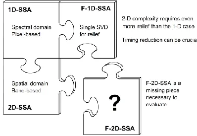
In some of our previous work, we have evaluated the singular spectrum analysis (SSA) [7] technique for feature extraction in HSI remote sensing. Basically, the SSA algorithm is able to decompose original 1-D signals into the main trend, oscillations and noise; therefore, initially we applied this technique for feature extraction in the spectral domain (applied to pixels) as 1D-SSA [8], which led to improved support vector machine (SVM) classification accuracy. Afterwards, we naturally extended this approach to the 2-D spatial domain (applied to spectral bands or images), introducing the 2D-SSA method plus a comprehensive benchmarking with the current state of the art in [9], where impressive results are achieved.
Fig. 1. F-2D-SSA inside the context of the SSA methods in hyperspectral remote sensing.
Given the potential of 2D-SSA, we find indispensable to introduce and evaluate a fast implementation of it. Actually, the 2D-SSA method, yet faster than 2D-EMD, still presents considerable computational complexity that makes crucial the introduction of computational relief and optimization. Therefore, with an increasing world-wide interest in mobile and embedded devices, accurate classification methods such as 2D-SSA are highly encouraged to optimize its implementation, reducing complexity and running time. Consequently, the main contribution presented in this paper is to propose a fast implementation for 2D-SSA, becoming a novel method, which is evaluated to show the superiority of its performance.
The remaining part of this manuscript is organized as follows. Section II starts with the basic mathematical background of the conventional 2D-SSA algorithm for feature extraction in HSI remote sensing, followed by our trick for fast implementation and the F-2D-SSA algorithm description. The experimental setup to compare both conventional and fast implementations, showing their differences under several scenarios in SVM classification, is presented in Section III. Finally, experimental results and further analysis are discussed in Section IV, leading to the concluding remarks drawn in Section V.
II. FAST IMPLEMENTATION F-2D-SSA
Derived from the basic SSA algorithm, the 2D-SSA method is an extension employed for 2-D signals or images [15, 16]. We already introduced and evaluated the 2D-SSA algorithm for feature extraction in HSI [9], where its conventional implementation is well-know and can be easily found in several of the cited works [9, 15, 16]. In the following, a brief summary is provided for clarity to the readers.
Let P2Dbe an image sized NxNy, a window
L
2Dis defined with dimensions L2DLxLy, where Lx[1,Nx] and] , 1
[ y
y N
L . With this window, a trajectory matrix X2DL2DK2D of the image P2D can be constructed (embedding stage),
SVD is then applied to the matrix X2D. This SVD is equivalent to an eigenvalue decomposition (EVD) of the matrix T
D D 2
2 X
X , which results in eigenvalues
1
2
L2D
and corresponding eigenvectors
D DD L L
L 2 2 2 , , , 2
1
u u u
U . Therefore, the trajectory matrix is decomposed in X2DX1X2XL2D where each
matrix
X
l is related to its corresponding eigenvalue, and can be defined byl l T D l T l l l
l u v v X u
X , 2 . (1)
The 2D-SSA algorithm basically consists of decomposing an imageP2D by SVD for a posterior reconstruction with only specific components, which is also known as grouping. In practical terms, the grouping stage consists of a multiplication derived from equations in (1), so combining both equations and selecting a single group namely tcontaining all the desired components, the reconstructed trajectory matrix is expressed as
Xt2DUt(X2DTUt)T UtUTtX2D, (2) with Ut as a matrix where each column is the eigenvector from each selected component. This selection of components is known
as Eigenvalue grouping (EVG). Please note that the resulting matrix
X
2tD from the grouping stage is not necessarily HbH type. In order to convert this resulting matrix to the reconstructed final image, it needs to be transformed first to an HbH-type matrix.This is done by an average procedure of the different values of Xt2Dthat contribute to the same element
i,j in the image P2D,known as a diagonal averaging [9]. Finally,
Z
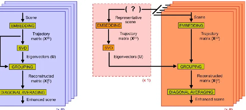
2D is the reconstructed image from the selected eigenvalue components.Fig. 2. Conventional application of 2D-SSA to a hyperspectral cube (band-based).
Despite the 2D-SSA method has been proven extremely effective in pixel classification, its band-based implementation forces to compute a complete SVD stage for every spectral band in the cube. This fact leads to remarkable computational complexity, which can also be reflected in large computation time. Nevertheless, given the shared configuration for each of the individual images in the
cube, the X2D construction is undertaken in the same parameters, where the eigenvectors from the SVD can be commonly applied to all the band images. This fact allows the fast implementation trick, relieving computational complexity by implementing a unique SVD stage, as explained in the following.
The difference introduced by our fast implementation is simply related to the common SVD stage, where the rest of stages, i.e. embedding, grouping and diagonal averaging are just the same, being applied individually. Fig. 3 shows a clear comparison between conventional and fast implementation. Therefore, in our proposed F-2D-SSA, the band-based (repetitive) sequence of SVD is no longer needed. Nevertheless, a single sequence including SVD is still required.
[image:5.612.104.517.515.700.2]Once the SVD stage implementation is reduced to a unique case, questions arise regarding what the appropriate SVD input is. From our point of view, the representative band scene to which the SVD is applied must possess the general characteristics of those scenes forming the hyperspectral cube. As all the scenes are indeed acquired by the same sensor, at the same time and in the same conditions, it is assumed that a scene resulting from the mean, or alternatively the median value from the scenes in the cube will contain adequately the properties of the whole data set, analogously to the 1-D case [14]. Therefore, suggesting the use of the mean (or median) image as SVD input, the implementation steps of F-2D-SSA in HSI are now listed in Algorithm 1, where experimental results are presented in Section IV to fully validate the effectiveness of the proposed F-2D-SSA algorithm.
Algorithm 1: F-2D-SSA in HSI
1) Initialization:
1.1 Input: hyperspectral cube with dimensionsNxNyB;
1.2 Configuration: Choose parameters window size L2D, EVG and representative scene. These will be used for all the spectral
scenes. It is suggested to use small/medium windows along with few eigenvalue components (1st, 1-2nd). For the representative scene, we propose to use the mean or median scene from the whole hyperspectral cube.
2) Find a unique set of eigenvalues for all the spectral bands:
2.1 Calculate the mean or median spectral scene from the cube. It will be the representative scene;
2.2 Embed the representative scene on a trajectory matrix X2Dusing L2D;
2.3 Perform EVD of the matrix X2DX2DTto obtain eigenvectors
LD
LD LD 2 2 2, ,
, 2
1
u u u
U ;
3) Apply 2D-SSA with the given eigenvectors to one spectral band or scene P2D (e.g. b=1):
3.1 Embed the current spectral scene on a trajectory matrix X2Dusing L2D;
3.2 Apply eq. (2) with the unique set of eigenvectors Uand the selected EVG (t) to obtain the reconstructedX2tD;
3.3 Perform diagonal averaging as in [9] to invert the embedding step and obtain the final reconstructed image Z2D.
5) Output: A new cube with dimensions NxNyB in which all spectral bands have been transformed by F-2D-SSA.
III. EXPERIMENTAL SETUP
In this paper, we propose an experimental setup similar to the one in [9], so we can compare both conventional 2D-SSA and F-2D-SSA in fair conditions to prove the advantage of the proposed fast implementation under the hardest situations. Undertaken in Matlab environment, comprehensive details about the data description and conditioning are presented below, along with the strategies for comparing methodologies and the configuration of the classifier employed (SVM).
A. Data Description and Conditioning
A total of three data sets are employed in our experiments. They are subscenes extracted from original and well-known hyperspectral images [17, 18] collected by two different sensors. These data sets are available to the public for remote sensing applications, and they include available ground truth allowing thus comprehensive analysis.
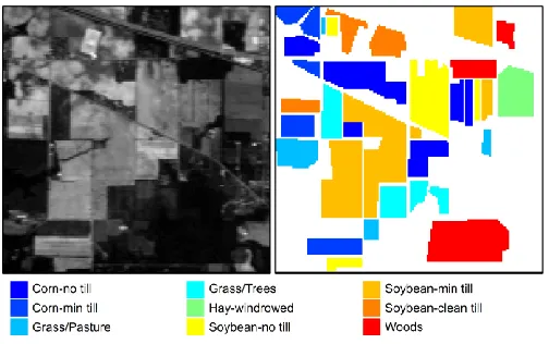
[image:7.612.180.432.485.643.2]First, the 92AV3C data set [17] in Fig. 4 was collected by the Airborne Visible/InfraRed Imaging Spectrometer (AVIRIS) [19] in Northwest Indiana, USA. This widely-used data set contains 220 spectral bands in the range from 400 to 2500 nm, with spatial dimensions of 145×145 pixels. However, the number of spectral bands is commonly reduced from 220 to 200 to avoid some noisy bands [9, 11, 20]. It contains 16 labeled classes related to agriculture, forest and vegetation, although it is usual to discard 7 classes with reduced number of samples available, as we do for consistency with previous studies [8, 9, 11, 20].
Second, the subscene Pavia University A (Pavia UA) taken in Pavia (North Italy) is used, where the data set was captured by the Reflective Optics System Imaging Spectrometer (ROSIS) [18, 21] and sized to 150×150 with a spatial resolution of 1.3 m. This urban image shown in Fig. 5 presents 115 bands in the spectral range from 430 to 860 nm, although only 103 bands are available, including 8 classes such as bitumen and asphalt among others.
[image:8.612.180.433.248.406.2]Third, Salinas C image shown in Fig. 6 was acquired by AVIRIS [18, 19] over the Salinas Valley in California, USA. Salinas C image is sized 150×150 with 224 spectral bands and a resolution of 3.7 m in the spatial domain. The initial 224 spectral bands are reduced to 204, due to water absorption and noise artifact. Its ground truth provides 9 labeled classes related to agriculture such as grapes, vineyards, broccoli and fallow.
Fig. 5. One band image at the wavelength of 521 nm (left) and the ground truth map (right) for the Pavia UA data set.
Fig.6. One band image at the wavelength of 667 nm (left) and the ground truth map (right) for the Salinas C data set.
B. Strategies for the 2D-SSA vs F-2D-SSA Comparison
[image:8.612.180.431.446.603.2]a decrease in computational complexity by F-2D-SSA, with reduced number of multiply-accumulates (MACs) and limited running time. In order to accomplish these two points, it is also important to evaluate the similarity of the features extracted by both methods and what an appropriate representative scene is for F-2D-SSA. Therefore, the comparison strategies developed in the experiments include similarity of extracted features, classification accuracy, analysis on the representative scene and computational complexity as detailed in Section IV.
C. Data Classification
Effectiveness in feature extraction is commonly measured by the accuracy achieved from the classifier in the experiments. To this end, the classification setup needs to be appropriate with relation to the current state of the art. Bearing that in mind, SVM has been proven to be very robust and adequate in multi-class classification [6, 20, 22]. Additionally, the wide use of SVM in recent years has led to many and easy-to-use libraries even for embedded implementations [23, 24]. Hence, SVM is employed as classifier for supervised learning in our experiments, using the LIBSVM library available in [25] that offers a user-friendly interface with Matlab environment. For the implementation of SVM, a Gaussian RBF kernel is adopted with several works supporting this selection [9, 11, 20], and a grid search is used every time in order to adequately tune the two key parameters from the RBF-SVM; the penalty c and the gamma γ.
Every experiment using each of the feature extraction methods along with the SVM classifier is repeated ten times with different training and testing subsets (no sample overlap allowed) so that the overall experiment holds notable statistical significance. The training and testing subsets are randomly obtained through stratified sampling with an equal sample rate of 5% in each class for training, using remainder samples for testing. Then, classification results from the testing samples in terms of the overall accuracy (OA) are averaged over the ten repetitions, providing the mean values. Further evaluations also provide the mean value of the average accuracy (AA) and the class-by-class accuracy (CBC). Moreover, the McNemar’s test of significance is also used as a performance measurement, where the Baseline case (use of original features) is introduced as a reference. Therefore, in our experiments McNemar’s test provides a parameter Z that, when Z > 1.96, indicates the evaluated method beats the Baseline case with proper statistical significance (confidence level of 95%). More information about McNemar’s test can be found in [26].
IV. RESULTS AND EVALUATIONS
some state-of-the-art techniques. Afterwards, we perform a brief analysis on the representative scene to be used as a SVD input. Finally, once proven the similarity between both implementations and their superiority over the rest of techniques, their computational complexity is evaluated in terms of MACs and running time to show the clear advantage of our F-2D-SSA over the conventional case.
A. Features Similarity
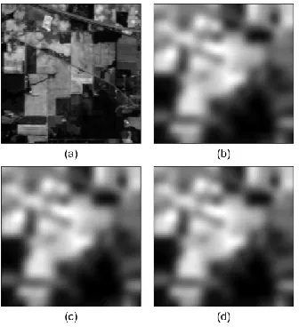
The possible effects derived from the implementation of a unique SVD and the use of a single set of eigenvectors in F-2D-SSA needs to be addressed in some way. Initially, we compare an original HSI scene (a band from 92AV3C at 667nm) with the resulting scenes from conventional 2D-SSA and F-2D-SSA (for both mean and median cases). This is shown in Fig. 7, where the three resulting scenes seem unnoticeable different.
[image:10.612.222.390.410.594.2]Now, the cosine distance is employed to objectively measure the difference between the proposed implementations. If the scenes being compared have similar trend, the cosine distance will detect it while other metrics such as the Euclidean distance would fail. Moreover, the cosine distance is not affected by scale and in practical terms lies in the range [0-1], making it appropriate in this context. In Table I, the mean cosine distance (comprising all spectral scenes in the cube) between the original scenes and the three 2D-SSA implementations, i.e. the conventional and the two fast implementations, is expressed for a wide range of configuration parameters. From this table, the similarity of the resulting features is clearly demonstrated.
Fig. 7. Application of 2D-SSA to a scene in HSI. (a) Original scene at 667 nm (b) conventional 2D-SSA implementation (c) F-2D-SSA mean-based implementation (d) F-2D-SSA median-based implementation, where L2D=10×10 and EVG=1st.
TABLE I
MEAN COSINE SIMILARITY SCORES TO QUANTIFY THE DIFFERENCE BETWEEN THE ORIGINAL AND RECONSTRUCTED SCENES BY 2D-SSA AND F-2D-SSA FROM THE 92AV3C DATA SET
Conventional SSA
L2D\EVG 1st 1-2nd 1-5th 1-10th
5×5 99.8996 99.9345 99.9746 99.9917
10×10 99.7999 99.8553 99.9216 99.9536
40×40 99.5288 99.6150 99.7105 99.7793
60×60 99.4519 99.5417 99.6456 99.7249
F-2D-SSA (mean)
L2D \EVG 1st 1-2nd 1-5th 1-10th
5×5 99.8995 99.9343 99.9745 99.9917
10×10 99.7996 99.8547 99.9212 99.9533
20×20 99.6728 99.7374 99.8326 99.8851
40×40 99.5313 99.5874 99.7075 99.7744
60×60 99.4586 99.5045 99.6226 99.6991
F-2D-SSA (median)
L2D \EVG 1st 1-2nd 1-5th 1-10th
5×5 99.8995 99.9341 99.9742 99.9916
10×10 99.7998 99.8546 99.9208 99.9531
20×20 99.6731 99.7368 99.8324 99.8835
40×40 99.5279 99.6054 99.7062 99.7769
60×60 99.4391 99.5307 99.6359 99.7131
B. Classification Accuracy Comparison
In order to evaluate the F-2D-SSA performance, we include classification results under the same conditions for the conventional 2D-SSA and the fast implementation using both mean and median values from the whole cube as representative scenes. The results are obtained for all previous configurations of window size L2D and EVG (5×5, 10×10, 20×20, 40×40 and 60×60, with an EVG comprising the 1st, the 1-2nd, the 1-5th and the 1-10th components) showing the best case and the average value from all settings.
As derived from Tables II-IV, F-2D-SSA is able to provide a very similar accuracy, where mean OA values fluctuate close to the conventional ones. For instance, in the 92AV3C data set, 95.66% and 95.82% are the accuracies from F-2D-SSA, compared to the conventional result of 95.71%. Similar outcome is obtained from Pavia UA (98.15% and 98.51% for 98.21%) and Salinas C (99.27% and 99.58% for 99.81%). This consistency is also reflected by the McNemar’s test parameter in brackets, having the Baseline case (original features) as reference.
TABLE II
MEAN OVERALL ACCURACY (%) AND MEAN MCNEMAR’S TEST [Z] FOR THE 92AV3C DATA SET USING 2D-SSA AND F-2D-SSA Method Best case Average from all configurations
L2D=10×10 EVG=1st
2D-SSA 95.71 [+31.4] 93.19 [+25.9]
F-2D-SSA (mean) 95.66 [+31.3] 93.50 [+26.5]
F-2D-SSA (median) 95.82 [+31.5] 93.44 [+26.4]
TABLE III
MEAN OVERALL ACCURACY (%) AND MEAN MCNEMAR’S TEST [Z] FOR THE PAVIA UA DATA SET USING 2D-SSA AND F-2D-SSA Method Best case Average from all configurations
L2D=5×5 EVG=1-2nd
2D-SSA 98.21 [+8.55] 96.99 [+3.91]
F-2D-SSA (mean) 98.15 [+8.20] 96.61 [+2.88]
F-2D-SSA (median) 98.51 [+9.69] 96.79 [+3.41]
TABLE IV
Method Best case Average from all configurations L2D=40×40 EVG=1-2nd
2D-SSA 99.81 [+13.6] 99.44 [+10.1]
F-2D-SSA (mean) 99.27 [+8.12] 99.40 [+9.72]
F-2D-SSA (median) 99.58 [+11.3] 99.38 [+9.47]
Additionally, CBC and AA values (from the best case) are provided in Tables V-VII to further compare the methods accuracy, where it can be checked in detail through the different land-cover classes.
TABLE V
MEAN CLASS-BY-CLASS ACCURACIES (%) FOR THE 92AV3C DATA SET OBTAINED FROM THE BASELINE, 2D-SSA AND F-2D-SSA (L2D=10×10, EVG=1ST)
APPROACHES AS WELL AS THE NUMBER OF SAMPLES (NOS) IN EACH CLASS Class NoS Baseline 2D-SSA F-2D-SSA (mean) F-2D-SSA (median)
1434 75.38 95.38 94.88 95.65 834 63.32 96.00 96.00 96.00 497 89.30 94.79 94.77 94.60 747 96.81 96.59 96.47 96.50 489 99.07 97.09 97.16 97.11 968 65.97 90.45 89.76 91.23 2468 81.10 96.54 96.92 96.60 614 69.97 93.86 93.84 93.67 1294 97.62 98.47 98.45 98.46 Average accuracy 82.06 95.46 95.36 95.54 Overall accuracy 81.26 95.71 95.66 95.82
TABLE VI
MEAN CLASS-BY-CLASS ACCURACIES (%) FOR THE PAVIA UA DATA SET OBTAINED FROM THE BASELINE, 2D-SSA AND F-2D-SSA (L2D=5×5, EVG=1-2ND)
APPROACHES AS WELL AS THE NUMBER OF SAMPLES (NOS) IN EACH CLASS
Class NoS Baseline 2D-SSA F-2D-SSA
(mean)
F-2D-SSA (median) 310 80.71 94.15 92.04 94.29 957 97.03 99.90 99.89 99.78 154 93.97 93.56 90.41 90.68 698 99.40 99.20 99.61 99.61 2559 96.76 98.98 99.53 99.55 860 93.15 95.21 94.98 96.56 854 95.86 98.19 97.37 97.78 293 100 99.21 99.03 99.21 Average accuracy 94.61 97.30 96.61 97.18 Overall accuracy 95.83 98.21 98.15 98.51
TABLE VII
MEAN CLASS-BY-CLASS ACCURACIES (%) FOR THE SALINAS C DATA SET OBTAINED FROM THE BASELINE, 2D-SSA AND F-2D-SSA (L2D=40×40, EVG=1-2ND)
APPROACHES AS WELL AS THE NUMBER OF SAMPLES (NOS) IN EACH CLASS
Class NoS Baseline 2D-SSA F-2D-SSA
(mean)
[image:12.612.187.428.260.405.2]1957 99.28 99.99 99.92 99.86 599 99.16 98.42 96.73 98.15 1155 96.92 99.29 97.96 99.04 1414 99.96 99.93 98.70 99.82 848 99.60 99.76 99.70 99.70 5890 99.47 99.90 99.89 99.87 159 07.28 98.61 92.98 92.52 Average accuracy 88.00 99.54 97.52 98.25 Overall accuracy 98.30 99.81 99.27 99.58
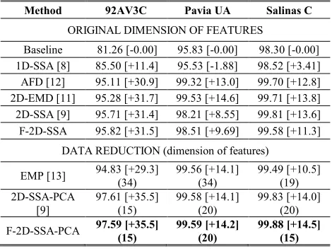
Given the classification accuracy achieved by the F-2D-SSA, now we place this performance in context with other state-of-the-art techniques. These techniques include not only using the original features (Baseline case), but also the 1D-SSA [8], the AFD [12], and the 2D-EMD [11] approaches, where in all of them the original dimensionality of features is preserved, so no data reduction is achieved. On the other hand, the EMP method [13] along with the combination of either 2D-SSA or F-2D-SSA with PCA [10] is evaluated for both feature extraction and data reduction. All the methods are implemented with the optimized parameters used in [9] showing the best result.
[image:13.612.189.424.539.715.2]Our proposal presents similar results as the conventional 2D-SSA; hence, it is proven to beat most of the techniques as shown in Table VIII, where only few cases provide higher accuracy (AFD, 2D-EMD and EMP for Pavia UA). Results from Table VIII are the best cases obtained in every method [9]. Therefore, 2D-SSA and F-2D-SSA are configured with L2D=10×10, EVG=1st, L2D=5×5,
EVG=1-2nd and L2D=40×40, EVG=1-2nd for 92AV3C, Pavia UA and Salinas C, respectively. Moreover, our fast implementation can also be combined with the PCA technique for data reduction. This combination was already evaluated in [9], so both the 2D-SSA-PCA previously, and now F-2D-SSA-PCA are able to exploit not only the spatial but also the spectral domain of HSI cubes. This combination achieves the best results from all the techniques evaluated, even though the number of features is reduced.
TABLE VIII
MEAN OVERALL ACCURACY (%) AND MEAN MCNEMAR’S TEST [Z] FROM THE DIFFERENT METHODS EVALUATED (BEST CASES)
Method 92AV3C Pavia UA Salinas C
ORIGINAL DIMENSION OF FEATURES
Baseline 81.26 [-0.00] 95.83 [-0.00] 98.30 [-0.00] 1D-SSA [8] 85.50 [+11.4] 95.53 [-1.88] 98.52 [+3.41] AFD [12] 95.11 [+30.9] 99.32 [+13.0] 99.70 [+12.8] 2D-EMD [11] 95.28 [+31.7] 99.53 [+14.6] 99.71 [+13.8] 2D-SSA [9] 95.71 [+31.4] 98.21 [+8.55] 99.81 [+13.6] F-2D-SSA 95.82 [+31.5] 98.51 [+9.69] 99.58 [+11.3]
DATA REDUCTION (dimension of features)
EMP [13] 94.83 [+29.3] (34) 99.56 [+14.1] (34) 99.49 [+10.5] (19) 2D-SSA-PCA [9] 97.61 [+35.5] (15) 99.58 [+14.1] (20) 99.83 [+14.0] (20) F-2D-SSA-PCA 97.59 [+35.5]
(15)
99.59 [+14.2] (20)
C. Analysis on the Representative Scene
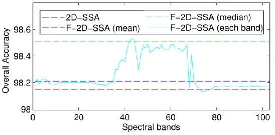
[image:14.612.175.448.206.352.2]Although the mean and median scenes from the whole HSI cube seem an appropriate input for F-2D-SSA, it is important to remark that other different options are possible. In order to bring some light to this issue, we briefly evaluate the performance of different inputs, in terms of OA. In fact, now we use every single spectral band in the cube as a representative scene to see how the classification accuracy does with relation to the new input.
Fig.8. Comparison of the OA for F-2D-SSA (L2D=10×10, EVG=1st) with each spectral band used as a representative scene for the 92AV3C data set.
In Fig. 8, the OA values obtained with the best configuration for the 92AV3C data set fluctuate for the different spectral bands used as inputs. As can be seen, most of the values are found between the F-2D-SSA (mean) and the F-2D-SSA (median) cases, which actually validates the use of the mean and median operators for obtaining a representative scene. On the other hand, it is also observed that the use of some specific bands can slightly increase (b=160-170) or degrade (b=40-50) the performance, yet all OA values are close to the conventional 2D-SSA case. A similar behavior is found for the other data sets (Fig. 9-10).
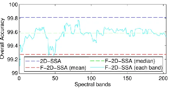
[image:14.612.176.450.518.653.2]Fig.10. Comparison of the OA of classification for F-2D-SSA (L2D=40×40, EVG=1-2nd) using each spectral band as a representative scene for Salinas C. From the behavior detected in Figs. 8-10, the median scene from the cubes seems to perform better than the mean scene. The explanation to this fact is simple; the median operator, unlike others such as the mean (average), is not mainly influenced by outliers, becoming more robust. In other words, given that HSI cubes usually contain noisy bands, the representative scene must avoid as much as possible noisy content, and the median operator smartly disregards noisy outliers. Actually, the median performs better than the majority of individual bands. Overall, we can suggest as a general recommendation the use of the median scene as input to the unique SVD in the fast implementations.
D. Computational Complexity
The proposed fast implementation reduces the SVD computation from hundreds of times to a single case that is applied to a representative scene. This fact directly translates into a saving factor in MACs related to the SVD step, as shown in this subsection, where we briefly analyze the computational complexity derived from each stage as follows:
In the embedding procedure, an original image is relocated into a trajectory matrix by means of a window with size L2D, however, no MACs are involved in this operation.
Then, the SVD stage takes places. This SVD can actually be computed by several algorithms described in the literature, where equivalent implementations based on EVD are also possible. As stated in [14], an equivalent EVD applied to
T D D
(
2)
2
X
X
S
is simpler ( (L2D)2 K2D + (L2D)3 )than the SVD complexity ( (L2D)2 K2D + L2D (K2D)2 + (K2D)3 )suggested in [27, 28], therefore, we work with this EVD complexity.
Afterwards, selection of components is made. The grouping stage is represented by the equation in (2), and even though
Finally, the last stage corresponding to the diagonal averaging procedure can be approximated as NxNy in a similar way as
we did in [14].
In Table IX, the computational complexity comparison between both implementations can be seen for all stages, where following Tables X-XII provide the actual number of MACs and the saving factor achieved for the three data sets, given four varied configurations. The complexity reduction in the SVD stage makes the fast implementation clearly easier than the conventional one, with minimum saving factors of 2 (halving the number of MACs) and even achieving a dramatically high reduction superior to 100 depending on the configuration case.
TABLE IX
COMPUTATIONAL COMPLEXITY IN THE DIFFERENT STAGES
Stage 2D-SSA F-2D-SSA Saving factor
Embed. N/A N/A 1
SVD [(L2D)2K2D+(L2D)3]×B [(L2D)2K2D+(L2D)3]×1 B Grouping [2L2DK2Dp]×B [2L2DK2Dp]×B 1
D. Av. [NxNy]×B [NxNy]×B 1
TABLE X
COMPUTATIONAL COMPLEXITY (MACS) AND SAVING FACTOR FOR THE 92AV3C DATA SET IN DIFFERENT CONFIGURATIONS
L2D= 5×5 5×5 60×60 60×60
EVG= 1st 1-10th 1st 1-10th
2D-SSA 2691e6 4481e6 28512e9 28608e9 F-2D-SSA 215e6 2005e6 153e9 249e9 Saving factor 12.5 2.23 186 115
TABLE XI
COMPUTATIONAL COMPLEXITY (MACS) AND SAVING FACTOR FOR THE PAVIA UA DATA SET IN DIFFERENT CONFIGURATIONS
L2D= 5×5 5×5 60×60 60×60
EVG= 1st 1-10th 1st 1-10th
2D-SSA 1486e6 2474e6 15866e9 15921e9 F-2D-SSA 125e6 1113e6 160e9 215e9 Saving factor 11.8 2.22 99.1 73.9
TABLE XII
COMPUTATIONAL COMPLEXITY (MACS) AND SAVING FACTOR FOR THE SALINAS C DATA SET IN DIFFERENT CONFIGURATIONS
L2D= 5×5 5×5 60×60 60×60
EVG= 1st 1-10th 1st 1-10th
2D-SSA 2943e6 4900e6 31424e9 31533e9 F-2D-SSA 235e6 2192e6 166e9 276e9 Saving factor 12.5 2.24 189 114
total timing can be reduced up to 60%, going from 496 to 194 s for the 92AV3C data set, where the timing reduction in percentage is similar for the other data sets.
TABLE XIII
APPROXIMATED RUNNING TIME REQUIRED FOR 2D-SSA AND F-2D-SSA FEATURE EXTRACTION IN 92AV3C DATA SET
Parameters 2D-SSA F-2D-SSA Reduction
L2D (s) (%)
5×5 19 18 1 5.26
10×10 31 28 3 9.68
20×20 69 58 11 15.9
40×40 244 137 107 43.9
60×60 496 194 302 60.9
TABLE XIV
APPROXIMATED RUNNING TIME REQUIRED FOR 2D-SSA AND F-2D-SSA FEATURE EXTRACTION IN PAVIA UA DATA SET Parameters
2D-SSA F-2D-SSA Reduction
L2D (s) (%)
5×5 10 10 0 0.00
10×10 17 15 2 11.8
20×20 38 32 6 15.8
40×40 137 77 60 43.8
60×60 282 113 169 59.9
TABLE XV
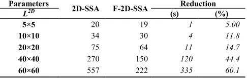
APPROXIMATED RUNNING TIME REQUIRED FOR 2D-SSA AND F-2D-SSA FEATURE EXTRACTION IN SALINAS C DATA SET Parameters
2D-SSA F-2D-SSA Reduction
L2D (s) (%)
5×5 20 19 1 5.00
10×10 34 30 4 11.8
20×20 75 64 11 14.7
40×40 270 150 120 44.4
60×60 557 222 335 60.1
[image:17.612.186.429.376.453.2]Fig.11. Running time (s) per stage and different L2D in conventional 2D-SSA for 92AV3C (left), Pavia UA (middle) and Salinas C (right).
Finally, a global comparison of the SSA methodologies, with classification accuracy and running time, is provided in Table XVI. The better performance of the 2-D methodologies in classification accuracy is clear, however, the pixel-based implementation from the 1-D cases involves a faster running time, basically because trajectory matrices in 1-D are smaller. Discussions can be derived from this fact, regarding what a good trade-off between accuracy and complexity can be when working with HSI. From our point of view, the classification accuracy comes first; looking for accuracies close to 100%, and that is probably the reason why most efforts in HSI are focused on the highest-accuracy problem. Nevertheless, complexity is a factor to bear in mind, making some implementations unfeasible. A good example is 2D-EMD in Salinas C, where it requires 1056 s, something incompatible with fast tasks. This issue points out our fast implementation importance and contribution.
TABLE XVI
GLOBAL COMPARISON ON MEAN OVERALL ACCURACY (%) AND RUNNING TIME FOR THE SSA METHODOLOGIES (BEST CASES) Method
92AV3C Pavia UA Salinas C
OA (%)
time (s)
OA (%)
time (s)
OA (%)
time (s)
Baseline 81.26 0 95.83 0 98.30 0
1D-SSA 85.50 13 95.53 7 98.52 13
F-1D-SSA 85.78 12 95.55 7 98.50 12
2D-SSA 95.71 31 98.21 10 99.81 270
F-2D-SSA 95.82 28 98.51 10 99.58 150
2D-SSA-PCA 97.61 31 99.58 10 99.83 270
F-2D-SSA-PCA 97.59 28 99.59 10 99.88 150
2D-EMD 95.28 936 99.53 688 99.71 1506
V. CONCLUSIONS
ACKNOWLEDGMENT
This work was supported by the National Natural Science Foundation of China (61272381, 61571141), Guangdong Provincial Application-oriented Technical Research and Development Special Fund Project (2015B010131017), Science and Technology Major Project of Education Department of Guangdong Province (2014KZDXM060), the Natural Science Foundation of Guangdong Province (2016A030311013, 2015A030313672) and International Scientific and Technological Cooperation Projects of Education Department of Guangdong Province (2015KGJHZ021).
REFERENCES
[1] T. Qiao, J. Ren, C. Craigie, J. Zabalza, C. Maltin, and S. Marshall, “Singular spectrum analysis for improving hyperspectral imaging based beef eating quality evaluation,” Computers and Electronics in Agriculture, 115: 21-25, 2015.
[2] T. Kelman, J. Ren, and S. Marshall, “Effective classification of Chinese tea samples in hyperspectral imaging,” Artificial Intelligence Research, 2(4): 87-96, 2013.
[3] G. Lu, and B. Fei, “Medical hyperspectral imaging: a review,” Journal of Biomedical Optics, 19(1), Jan. 2014.
[4] M. Sun, D. Zhang, Z. Wang, J. Ren, B. Chai, and J. Zhou, "What's Wrong with Murals at Mogao Grottoes: a Near-Infrared Hyperspectral Image Method," Scientific Reports, 5: Article number 14371, 2015.
[5] J. Ren, J. Zabalza, S. Marshall and J. Zheng, “Effective feature extraction and data reduction with hyperspectral imaging in remote sensing,” IEEE Signal Processing Magazine, 31(4): 149-154, Jul. 2014
[6] L. Fang, S. Li, W. Duan, J. Ren, J. Atli Benediktsson, “Classification of hyperspectral images by exploiting spectral-spatial information of superpixel via multiple kernels,” IEEE Trans. Geoscience and Remote Sensing, 53(12): 6663-6674, 2015
[7] N. Golyandina, A. Zhigljavsky, Singular spectrum analysis for time series, Springer, 2013.
[8] J. Zabalza, J. Ren, Z. Wang, S. Marshall, and J. Wang, “Singular spectrum analysis for effective feature extraction in hyperspectral imaging,” IEEE Geoscience and Remote Sensing Letters, 11(11): 1886-1890, 2014.
[9] J. Zabalza, J. Ren, J. Han, H. Zhao, S. Li, and S. Marshall, “Novel two-dimensional singular spectrum analysis for effective feature extraction and data classification in hyperspectral imaging,” IEEE Transactions on Geoscience and Remote Sensing, 53(8): 4418-4433, Aug. 2015.
[10] C. Rodarmel, and J. Shan, “Principal component analysis for hyperspectral image classification,” Surveying and Land Information Science 62(2): 115-122, 2002.
[11] B. Demir, and S. Ertürk, “Empirical mode decomposition of hyperspectral images for support vector machine classification,” IEEE Transactions on Geoscience and Remote Sensing, 48(11): 4071-4084, 2010.
[12] R. D. Phillips, C. E. Blinn, L. T. Watson, and R. H. Wynne, “An adaptive noise-filtering algorithm for AVIRIS data with implications for classification accuracy,” IEEE Transactions on Geoscience and Remote Sensing, 47(9): 3168-3179, Sep. 2009.
[14] J. Zabalza, J. Ren, Z. Wang, H. Zhao, J. Wang, and S. Marshall, “Fast implementation of singular spectrum analysis for effective feature extraction in hyperspectral imaging,” IEEE Journal of Selected Topics in Earth Observation and Remote Sensing, vol. 8, no. 6, pp. 2845-2853, Jun. 2015.
[15] N. Golyandina, and K. D. Usevich, “2D-extension of singular spectrum analysis: algorithm and elements of theory,” Matrix Methods: Theory, Algorithms, Applications World Scientific: 449-473. 2010.
[16] L. J. Rodrıguez-Aragón, and A. Zhigljavsky, “Singular spectrum analysis for image processing,” Statistics and Its Interface, 3: 419-426. 2010. [17] Pursue's university multispec site: June 12, 1992 aviris image Indian Pine Test Site [Online]. Available:
https://engineering.purdue.edu/~biehl/MultiSpec/hyperspectral.html.
[18] Hyperspectral Remote Sensing Scenes [Online]. Available: http://www.ehu.es/ccwintco/index.php/Hyperspectral_Remote_Sensing_Scenes.
[19] R. O. Green et al, “Imaging spectroscopy and the airborne visible/infrared imaging spectrometer (AVIRIS),” Remote Sensing Environment 65:227-248 Elsevier Science Inc., 1998.
[20] R. Archibald and G. Fann. “Feature selection and classification of hyperspectral images with support vector machines.” IEEE Geoscience and Remote Sensing Letters, 4(4), Oct. 2007.
[21] S. Holzwarth et al. “HySens - DAIS 7915/ ROSIS Imaging Spectrometers at DLR,” Presented at the 3rd EARSeL Workshop on Imaging Spectroscopy, Herrsching, 13-16 May 2003.
[22] G. Mountrakis, J. Im, and C. Ogole, “Support vector machines in remote sensing: a review,” ISPRS Journal of Photogrammetry and Remote Sensing, 66:247-259, 2011.
[23] J. Zabalza, J. Ren, C. Clemente, G. Di Caterina, and J.J. Soraghan, “Embedded SVM on TMS320C6713 for signal prediction in classification and regression applications,” in 5th European DSP Education and Research Conf., Amsterdam, Sep. 2012.
[24] J. Zabalza, C. Clemente, G. Di Caterina, J. Ren, J. J. Soraghan, and S. Marshal, “Robust PCA micro-Doppler classification using SVM on embedded systems,” IEEE Transactions on Aerospace and Electronic Systems, 50(3), Jul. 2014.
[25] Chih-Chung Chang and Chih-Jen Lin, LIBSVM: a library for support vector machines. ACM Transactions on Intelligent Systems and Technology, 2(3): 27 pages, 2011. Software available at http://www.csie.ntu.edu.tw/~cjlin/libsvm.
[26] G. M. Foody, “Thematic map comparison: Evaluating the statistical significance of differences in classification accuracy,” Photogramm. Eng. Remote Sens., 70(5): 627–633, May 2004.