City, University of London Institutional Repository
Citation
:
Sax, O. O., Sfondrini, A. & Stefanski, B. (2015). Integrability and the conformal field theory of the Higgs branch. Journal of High Energy Physics, 2015(6), p. 103. doi: 10.1007/JHEP06(2015)103This is the published version of the paper.
This version of the publication may differ from the final published
version.
Permanent repository link:
http://openaccess.city.ac.uk/12541/Link to published version
:
http://dx.doi.org/10.1007/JHEP06(2015)103Copyright and reuse:
City Research Online aims to make research
outputs of City, University of London available to a wider audience.
Copyright and Moral Rights remain with the author(s) and/or copyright
holders. URLs from City Research Online may be freely distributed and
linked to.
JHEP06(2015)103
Published for SISSA by SpringerReceived: November 28, 2014 Revised: May 7, 2015 Accepted:May 11, 2015 Published: June 16, 2015
Integrability and the conformal field theory of the
Higgs branch
Olof Ohlsson Sax,a Alessandro Sfondrinib and Bogdan Stefa´nski Jr.c
aTheoretical Physics, The Blackett Laboratory, Imperial College,
London, SW7 2AZ U.K.
bInstitut f¨ur Mathematik und Institut f¨ur Physik, Humboldt-Universit¨at zu Berlin, IRIS Geb¨aude,
Zum Grossen Windkanal 6, Berlin, 12489 Germany cCentre for Mathematical Science, City University London,
Northampton Square, London, EC1V 0HB U.K. E-mail: [email protected],
Abstract: In the context of the AdS3/CFT2 correspondence, we investigate the Higgs
branch CFT2. Witten showed that states localised near the small instanton singularity can be described in terms of vector multiplet variables. This theory has a planar, weak-coupling limit, in which anomalous dimensions of single-trace composite operators can be calculated. At one loop, the calculation reduces to finding the spectrum of a spin-chain with nearest-neighbour interactions. This CFT2 spin-chain matches precisely the one that was previously found as the weak-coupling limit of the integrable system describing the AdS3 side of the duality. We compute the one-loop dilatation operator in a non-trivial compact subsector and show that it corresponds to an integrable spin-chain Hamiltonian. This provides the first direct evidence of integrability on the CFT2 side of the correspondence.
Keywords: AdS-CFT Correspondence, 1/N Expansion
JHEP06(2015)103
Contents
1 Introduction 1
2 The D1-D5 system 4
2.1 Field content in the UV 5
2.2 Two-dimensional action by dimensional reduction 5
3 Effective action at the origin of the Higgs branch 7
4 Superconformal representations of the fields 10
4.1 The u(1,1|2) superalgebra 10
4.2 psu(1,1|2)L⊕psu(1,1|2)R decomposition of the fields 10
4.3 Spin-chain states 12
5 One-loop dilatation operator in the so(4) sector 13
5.1 “One-loop” Feynman diagrams 14
5.2 Computation of one-loop dilatation operator 16
6 Conclusions 18
A Gamma matrices 20
B G-functions 21
C Regularisation of Feynman diagrams 22
1 Introduction
The AdS/CFT correspondence [1–3] can be understood quantitatively through integrabil-ity methods in certain classes of AdS5/CFT4 and AdS4/CFT3 dual pairs. Reviews of this approach and references to the literature can be found in [4, 5]. Superstrings on AdS3 backgrounds with 16 supersymmetries are known to be classically integrable [6–8], and so one may wonder whether integrability underlies the AdS3/CFT2 correspondence.1 Re-cently, we have found the complete non-perturbative world-sheet integrable S matrix of string theory on such AdS3 backgrounds, including the hitherto unaccounted for massless modes [11–14].2 It appears now very likely that the AdS3/CFT2 correspondence with 16
1For a review of the generalities of the AdS
3/CFT2correspondence see [9]. Some aspects of the
integra-bility approach to AdS3/CFT2 have been recently reviewed in [10]. 2For some early work on integrability in the context of AdS
JHEP06(2015)103
supersymmetries is described, in the planar limit [17], through a holographic quantumintegrable system.
As a consequence, there exists an all-loop Bethe Ansatz (BA) whose solutions deter-mine the closed-string spectrum in these backgrounds [6, 18–21].3 It is known that this BA, in the weak-coupling limit, encodes the energy spectrum of an integrable spin chain with local interactions [18, 21, 22]. Based on experience with higher-dimensional holo-graphic integrability, this spin-chain is believed to describe the large-curvature or small ’t Hooft-coupling limit of a discretised string world-sheet.
In higher-dimensional examples of integrable holography the local integrable spin-chain emerges in perturbative gauge theory calculations of anomalous dimensions of single-trace operators, as first shown in [23]. The relation between the spin-chain and perturbative gauge theory gives strong evidence of integrability of the dual pair at small ’t Hooft cou-pling. In practice it also provides physical input and a rich testing ground for the weak-coupling limit of the non-perturbative quantum integrable system. Therefore, identifying how the spin-chain constructed in [18, 21, 22] emerges on the gauge theory side of the AdS3/CFT2 correspondence is a key outstanding problem.
The AdS3/CFT2 correspondence is different in a number of important ways from its higher-dimensional, higher-supersymmetric cousins. Firstly, unlike N = 4 super-Yang-Mills [24] or ABJM theory [25], the two-dimensional UV gauge theory is not conformal: the gauge coupling is dimensionful and the CFT2 appears as the IR fixed-point of renor-malisation group flow. Secondly, the AdS3/CFT2 dual pair has a large moduli space [26], while the higher-dimensional duals are parametrised (in the planar limit) only by the value of λ — the ’t Hooft coupling. Thirdly, the two-dimensional UV gauge theory has, in addition to the (adjoint-valued) gauge vector multiplet, a number of (fundamental- and adjoint-valued) hypermultiplets.
The moduli space of the two-dimensional UV gauge theory has two branches: the Coulomb branch and the Higgs branch, which are parametrised by non-zero expectation values of the scalars in vector multiplets and hypermultiplets, respectively. The moduli space metric in the IR is closely related to the UV one because of supersymmetry. The gauge coupling is part of a vector multiplet [27] and so the moduli space metric receives quantum corrections only on the Coulomb branch [28]. On the other hand the Fayet-Iliopoulos (FI) parameters [29] and theta angles can be promoted to hypermultiplets and so that they can appear in the Higgs branch moduli space metric [28]. Both sets of quantum corrections can be computed exactly because of supersymetry.
Maldacena [1] conjectured that the IR Higgs-branch CFT2 is dual to string theory on AdS3. From the string theory point of view this is very natural: the AdS3 background emerges as the near-horizon limit of a stack of Nc D1- and Nf D5-branes, with the two-dimensional U(Nc) gauge theory living on the D1-branes. In this UV description the Higgs branch parametrises the motion of the D1-branes inside the D5-branes, while on the Coulomb branch the D1-branes separate from the D5-branes.
3The original conjecture for the BA [6,18] was put forward formassivemodes only. Later, it was found
JHEP06(2015)103
An equivalent description of the Higgs branch is provided by the re-combination processof the D-branes as an instanton [30]. The D1-branes are absorbed into the D5-branes forming an instanton (of instanton number Nc) in the SU(Nf) gauge theory living on the D5-branes. The low-energy physics [30] matches precisely the ADHM description of instanton moduli space [31]. Since the moduli-space metric is protected by supersymmetry (it is in fact hyper-K¨ahler), the ADHM sigma-model gives a good description of the Higgs branch CFT2 for generic instanton configurations.
However when the size of the instantons shrinks to zero the moduli-space metric be-comes singular. Therefore, the CFT2 states whose wave-function is peaked around such configurations are not well described in terms of a sigma model. There is an alternative description of such states, which can be obtained from the UV gauge-theory Lagrangian by dropping the kinetic terms of the vector multiplet and integrating out the fundamental-valued hypermultiplets, yielding an effective action [32,33]. This procedure produces new, non-local kinetic terms and interactions for the vector multiplet fields. As a result, such fields no longer have canonical dimensions, rather they have geometric scaling dimensions. The dynamical fields that describe the localised states are adjoint-valued vector multiplets and hypermultiplets, with 1/Nf being the effective coupling constant.
In this paper we investigate the CFT2 states localised near the small-instanton sin-gularity using the description given in [32, 33]. The gauge-invariant operators in this sub-sector of the CFT2 can be written in terms of single- and multi-trace operators in-volving the vector multiplets and adjoint hypermultiplets. We show that, in the large Nc limit, the perturbation series re-arranges itself into a ’t Hooft like expansion inλ≡Nc/Nf with non-planar corrections suppressed by factors of 1/N2
c. As a result, in the planar limit the computation of anomalous dimensions of gauge invariant operators can be reduced to the the spectral problem of a periodic spin-chain with local interactions, much like was found for N = 4 SYM [23]. In a closed so(4) sub-sector of the CFT2 we calculate the one-loop anomalous dimension of single-trace operators in the planar limit (Nc ≫ 1) at small ’t Hooft coupling Nc/Nf ≪ 1. We show that the resulting computation reduces in the conventional way [23] to calculating the energy spectrum of an integrable spin-chain. As far as we are aware, this constitutes the first direct evidence of integrability on the CFT side of the duality.
In previous works [11,18,21,22], we have constructed an integrable worldsheet S ma-trix which can be used to calculate the perturbative closed string spectrum to all orders in the string tension on the AdS3side. Using this construction, the weakly-coupled spin-chain limit of the integrable system was obtained [18, 22]. The representations that appear in this spin-chain are precisely the same as the ones that we find in the spin-chain descrip-tion of the localised states of the CFT2 that we find in this paper. Further, in the so(4) sub-sector the dilatation operators of the AdS3 and CFT2 agree. These results lead us to suggest that we should identify the perturbative closed string spectrum of the pure R-R AdS3 theory with the CFT2 states localised near the small instanton singularity.
JHEP06(2015)103
we review the description of the CFT2 states localised near the small-instanton singularitygiven in [32,33]. In section 4we show how the field content of that theory fits into repre-sentations of psu(1,1|2)2, which is the rigid part of the smallN = (4,4) super-conformal algebra, and how such fields are represented in a spin-chain that matches the one intro-duced in [18,22]. In section 5we compute the one-loop dilatation operator in the bosonic
so(4) subsector of the theory, showing that it corresponds to an integrable Hamiltonian. We conclude in section6 and relegate some technical material to the appendices.
2 The D1-D5 system
The UV description of the dual pair is encoded in the dynamics of the open strings ending on a stack of D1 and D5-branes,
Nf D5-branes: 012345,
Nc D1-branes: 01,
with the directions 2345 compactified on a four-torus [1]. The D1- and D5-branes separately preserve supersymmetry corresponding to N = (8,8) in two dimensions. However, the intersection of the two stacks of branes only preserve N = (4,4). Open strings stretching between the branes give rise to several multiplets of this symmetry. The D1-D1 strings correspond to an N = (8,8) U(Nc) vector multiplet, which splits into an N = (4,4) vector multiplet and an adjoint hypermultiplet. The D1-D5 strings give bi-fundamental U(Nc)×U(Nf) hypermultiplets. Finally, the D5-D5 strings give an N = (8,8) U(Nf) vector multiplet. In the UV we will take the volume of the 2345 directions to be large. As a result, from the 1+1 dimensional point of view, the D5-D5 strings correspond to non-normalisable modes. Their kinetic terms come with a factor of the 2345 volume and so can be decoupled; the U(Nf) symmetry becomes global. Furthermore, the center-of-mass U(1) vector multiplet also decouples and the gauge group is given by SU(Nc).
The two-dimensional N = (4,4) multiplets can be obtained by dimensional reduc-tion of the corresponding six-dimensional N = (1,0) multiplets. The six-dimensional supersymmetry algebra has an R-symmetry that we will denote by su(2)•.4 Upon reduc-tion to two dimension we get an addireduc-tional su(2)L⊕su(2)R symmetry corresponding to
rotations in the four compact dimensions. We will also introduce an additional su(2)◦ symmetry under which only the fields in the adjoint hypermultiplet transform. In the brane-system, thesu(2)L⊕su(2)Rsymmetry corresponds to rotations in the directions 6–9,
while su(2)•⊕su(2)◦ gives rotations in the directions 2–5.
In the IR the theory has a small N = (4,4) superconformal symmetry. The Lie-superalgebra part of this symmetry algebra is given by psu(1,1|2)2. Here su(2)
L⊕su(2)R
plays the role of the R-symmetry, i.e., the two su(2) algebras insidepsu(1,1|2)2 [32]. The
4This notation will be useful to make contact with the isometries of AdS
3 ×S3 ×T4 as described
JHEP06(2015)103
algebrasu(2)• acts onpsu(1,1|2)2 as an outer automorphism, whilesu(2)◦ commutes withthe other symmetries.5
2.1 Field content in the UV
The vector multiplet consists of the gauge field Aµ, two left-moving fermions ψαLa˙, two
right-moving fermions ψα˙a˙
R , four scalars φαα˙ and three auxiliary fields Da˙
˙
b. Under the
global symmetries the fields transform as
su(2)L su(2)R su(2)• su(2)◦
Aµ 1 1 1 1
Da˙b˙ 1 1 3 1
φαα˙ 2 2 1 1
ψLαa˙ 1 2 2 1
ψRα˙a˙ 2 1 2 1
The fundamental hypermultiplet contains two complex scalarsHa˙, a doublet of left-moving fermionsλαL˙, a doublet of right-moving fermionsλ
α
R, as well as two auxiliary complex scalars
Fa˙. The charges of these fields are given by
su(2)L su(2)R su(2)• su(2)◦
Ha˙ 1 1 2 1
Fa˙ 1 1 2 1
λαL˙ 2 1 1 1
λα
R 1 2 1 1
The field content of the adjoint hypermultiplet is essentially the same as above , but can be written in terms of real fields by having the full multiplet transforming as a doublet under the global symmetrysu(2)◦. We denote the scalars byTaa˙, the fermions byχαaL˙ and
χαa
R and the auxiliary field by Gaa˙. The corresponding charges are given by
su(2)L su(2)R su(2)• su(2)◦
Taa˙ 1 1 2 2
Gaa˙ 1 1 2 2
χαaL˙ 2 1 1 2
χαa
R 1 2 1 2
2.2 Two-dimensional action by dimensional reduction
To obtain the Lagrangian of the two-dimensional UV field theory one can start with six-dimensional supersymmetric Yang-Mills theory and six-dimensionally reduce to two dimen-sions [24]. In six dimensions, the fermions in the vector multiplet satisfy the symplectic
5Our index conventions are as follows. We indicateso(1,1) chiralities by L and R. For the IR R-symmetry
so(4) algebra we hence writeso(4) =su(2)L⊕su(2)R, withsu(2)L,R⊂psu(1,1|2)L,Rand we represent the
JHEP06(2015)103
Majorana condition(ψa˙)∗ =Bǫa˙b˙ψ ˙
b, (2.1)
and are chiral
Γ012345ψa˙ = +ψa˙. (2.2)
The Lagrangian for the vector multiplet is
L6D
V =− 1
4trFµνF µν+ i
2tr ¯ψa˙∇/ψ ˙
a+1
2trDa˙b˙D ˙
ab˙. (2.3)
The hypermultiplet fermionλis complex and anti-chiral
Γ012345λ=−λ . (2.4)
The Lagrangian for the hypermultiplet and its couplings to the vector multiplet is
L6D
H =− 1 2∇µH
†
˙
a∇µHa˙+iλ /¯∇λ+iH †
˙
aψ¯a˙λ−iλψ¯ a˙Ha˙+ 1 2F
†
˙
aFa˙+ 1 2H
†
˙
aDa˙
˙
bH
˙
a. (2.5)
Above we have written the Lagrangian for a hypermultiplet transforming in the fundamen-tal representation of the gauge group. We will write the Lagrangian for the adjoint-valued hypermultiplets in its two-dimensional form below.
When we dimensionally reduce from six to two dimensions the so(1,5) Lorentz sym-metry is broken toso(1,1)⊕so(4) which we write asso(1,1)⊕su(2)L⊕su(2)R. The gauge
field then splits into a two-dimensional gauge fieldAµ and four real scalars φαα˙ that form a vector ofso(4).
Dimensionally reducing the kinetic term for the anti-chiral fermionλto two dimensions we find
iλ /¯∂λ=iλ†C /∂λ→iλ†∂tλ+iλ†γˆ2345∂xλ. (2.6)
Our gamma-matrix conventions can be found in appendixA. From this expression we see that worldsheet chirality is correlated withso(4) chirality. Hence, we split the fermionλas
λ→λαL˙ +λ
α
R (2.7)
so that the kinetic term becomes
iλ†Lα˙(∂t+∂x)λαL˙ +iλ
†
Rα(∂t−∂x)λαR. (2.8)
The fermion ψa˙ in the vector multiplet is chiral. The same sort of calculation as above therefore gives
iψ¯a˙∂ψ/ a˙ →iψ†Lαa˙(∂t+∂x)ψ
αa˙
L +iψ
†
Rα˙a˙(∂t−∂x)ψ
˙
αa˙
R . (2.9)
The full Lagrangian for the two-dimensional vector multiplet is then given by
LV = tr
−1 4FµνF
µν−1 2∂µφ
αα˙∂µφα
˙
α+iψL†αa˙∇+ψαLa˙+iψ
†
Rα˙a˙∇−ψαR˙a˙
−14[φαα˙, φββ˙][φαα˙, φββ˙] +iψL†αa˙[φαα˙, ψRα˙a˙] +iψ
†
Rα˙a˙[φαα˙, ψLαa˙] +
1 2Da˙b˙Da˙
˙
b
.
JHEP06(2015)103
The Lagrangian for the fundamental hypermultiplet and its couplings to the vectormulti-plet then takes the form
LH =− 1 2∇µH
†
˙
a∇µHa˙+iλ †
Lα˙∇+λαL˙ +iλ
†
Rα∇−λ
α R+ 1 2F † ˙
aFa˙
−1 2H
†
˙
aφαα˙φαα˙Ha˙ +iλ†Lα˙φ
αα˙λ
Rα+iλ†Rαφ
αα˙λ
Lα˙ + 1 2H
†
˙
aDa˙
˙
bH
˙
b
+iHa†˙ψL†αa˙λRα+iHa†˙ψ
†α˙a˙
R λLα˙ −iλ†Lα˙ψ
˙
αa˙
R Ha˙ −iλ
†
Rαψ
αa˙
L Ha˙,
(2.11)
and the Lagrangian for the adjoint hypermultiplet the form
LT = tr
−12∇µTaa˙∇µTaa˙ +iχ†Lαa˙ ∇+χ
˙
αa
L +iχ
†
Rαa∇−χαaR +
1 2Gaa˙G
aa˙
−1
2[φαα˙, Taa˙][φ
αα˙, Taa˙] +iχ†
Rαa˙ [φ
αα˙, χ
Lαa] +iχ†Lαa[φ
αα˙, χ
Rα˙a]
+1 2Taa˙[D
˙
ab˙, Ta
˙
b] +iχ †
Lαa˙ [ψαR˙a˙, T
a
˙
a] +iχ†Rαa[ψαLa˙, T
a ˙ a] . (2.12)
We can now write the full two-dimensional UV Lagrangian as
LUV(φ, H, T) = 1 g2
YM
LV(φ) +LH(H, φ) +LT(T, φ). (2.13)
In the above equation we write φ, H and T as short-hand for all fields in these super-multiplets, and the dependence of LUV on gYM has been explicitly written out.
3 Effective action at the origin of the Higgs branch
In the previous section we wrote down the two-dimensional N = (4,4) SYM Lagrangian LUV for the D1-D5 system in the UV. Since gYM is dimensionful, this theory flows. As explained in [32], the IR is described by two decoupled CFTs: one corresponding to the Coulomb branch and the other to the Higgs branch. Within the context of AdS/CFT we will be interested in the Higgs branch (4,4) CFT2 [1]. Witten [32] made a proposal for how to describe this CFT2. The argument is further discussed in [33] and we review it presently. SincegYM is dimensionful,LV is irrelevant and can be dropped while flowing to the IR. The IR Lagrangian is then
LIR(φ, H, T) =LH(H, φ) +LT(T, φ). (3.1)
LIRis conformal provided we assign the fields in the vector multiplet the following geometric scaling dimensions [32]
dim(A) = 1, dim(φ) = 1, dim(ψ) = 3/2, dim(D) = 2. (3.2)
The fields in the hypermultiplets retain their canonical dimensions.
JHEP06(2015)103
out the non-dynamical vector multiplet fields in LIR [33]. However, near the origin of theHiggs branch, this moduli space has a singularity. The degrees of freedom describing states localised near the origin of the Higgs branch are the adjoint-valued vector multiplet and hypermultiplet fields [32,33]. The physics of these localised degrees of freedom is obtained by integrating out from LIR the fundamental hypermultipletsH
Z
DφDTDH eiRd2xLIR =
Z
DφDT eiRd2x(NfLeff(φ)+LT(T,φ)). (3.3)
Since the adjoint and fundamental hypermultiplets do not couple to one another inLIR,LT remains unchanged. On the other hand for the vector multiplet we see that this procedure results in what Witten called an “induced gauge theory”: the vector multiplet acquires kinetic terms coming exclusively from performing the path integral over the fundamental hypermultiplets. In addition to these kinetic terms, the vector multiplet fields also have higher-order (in the number of fields) interactions determined by the integrating-out proce-dure. We denote the resulting vector multiplet action byLeff(φ); the Lagrangian governing the adjoint-valued fields is then
NfLeff(φ) +LT(T, φ). (3.4)
Notice that Leff(φ) appears with an overall factor of Nf which comes from the sum over flavours in the fundamental hypermultiplet loop.6 In the remainder of this section we
discuss in more detail Leff(φ) and how it may be used to perform calculations in the localised sector of theCF T2.
As we mentioned above, integrating out the fundamentals results in the vector multiplet fields becoming dynamical: Leff contains non-standard kinetic terms that account for the scaling dimensions given in equation (3.2). Conformal invariance then dictates the form of the two-point functions of the fields in the vector multiplet. For example, the dimension one scalar φhas a two-point function of the form
hφαα˙(x)φββ˙(y)i= Cǫ αβǫα˙β˙
|x−y|2, (3.5)
whereC is a normalisation constant.
The non-standard kinetic terms in Leff modify the dynamical degrees of freedom in the vector multiplet. In a theory with a conventional kinetic term, the two-dimensional gauge field Aµ carries no physical degrees of freedom. In Leff, on the other hand, Aµ has a non-standard kinetic term, and so the gauge field will now carry one degree of freedom. Similarly, the field Dab is auxiliary in the standard Lagrangian, but is a physical field of dimension 2 in the effective theory. N = (4,4) supersymmetry [37], should be powerful enough to determine the kinetic terms of the full vector multiplet from the kinetic term of the scalarsφ.7
6This action is reminiscent of the Coulomb branch action. The relationship between the two is discussed
in refs. [33,36].
JHEP06(2015)103
Witten’s description of the states localised near the singularity of the Higgs branch interms ofLeff simplifies whenNc= 1. In that case, it was argued in [33] that the description reduces to a level Nf supersymmetric SU(2) WZW model coupled to a charged scalar of chargeQ= (Nf−1)
p
2/Nf. In [33], it is argued that the fieldsφaa˙ are composite operators
φαα˙ =e√2/Nfϕuαα˙, (3.6)
where u is the fundamental field of the WZW model and ϕ is the charged scalar. Using the well-known OPEs of u andϕ one finds
φαα˙(x)φββ˙(y)∼ ǫ αβǫα˙β˙
|x−y|2−
5 2Nf
. (3.7)
This is consistent with our expression (3.5) in the large Nf limit.
The effective Lagrangian Leff also contains higher-order terms in the vector multiplet fields. We now describe how these interactions arise from LIR and the integrating-out procedure. In the Lagrangian LIR there are interaction vertices involving fields from the fundamental hypermultiplet and fields from the vector multiplet. Hence, the fundamental hypermultiplet mediates interactions between fields of the vector multiplet. Let us look at an example which will be important in section5. The vector multiplet scalar fieldφappears quadratically in the Lagrangian LIR. It interacts with the fundamental hypermultiplet through the termsH†φφH andλ†φλ, see equation (2.11). As a result, when performing the path integral over the fieldsHandλin equation (3.3) the resulting functional determinant will yield a non-local quartic effective vertex for φ. This is most transparent in terms of Feynman diagrams:8
= + . (3.8)
Here the double lines correspond toφ, the single solid lines toHand the dashed lines toλ. The fat dot stands for the effective vertex, while the diagrams on the right hand side can be written using the Feynman rules of LIR. Equation (3.8) provides us with an efficient way to compute diagrams involving effective vertices. This information, together with the propagator of equation (3.5) is all we will need to study the one loop mixing of operators in section 5. This kind of diagrammatics, as well as the scaling inNf of equation (3.4), is reminiscent of large-N models [40].
We conclude this section by noting that there are two parameters in the theory: the number of flavours Nf and the number of colours Nc. In the effective Lagrangian, Nf plays the role of the Yang-Mills coupling 1/gYM2 . Hence, it is natural to consider the weakly coupled ’t Hooft limit, whereNf, Nc → ∞ withNc/Nf ≪1 fixed.
8The effective vertex has a particularly simple expression in terms of Feynman diagrams because the
LagrangianLIRis quadratic in the fieldsλandHthat are integrated out. Hence, the functional integration
JHEP06(2015)103
4 Superconformal representations of the fields
In this section we show how the field content of the theory described above fits in repre-sentations of psu(1,1|2)2, which is the rigid part of the small N = (4,4) superconformal algebra, and how these match with the representations used in the spin-chain constructed in [18,22]. We start by briefly reviewing the u(1,1|2) superalgebra.
4.1 The u(1,1|2) superalgebra
Theu(1,1|2) superalgebra consists of thesu(2) R-symmetry generatorsRab, the translation P, the superchargesQaand ˙Qa, the dilatationD, the special conformal transformationK, the conformal superchargesSa and ˙Sa, the central chargeC and the hyperchargeB. We write thesu(2) commutation relations as
[Jab,Rc] = +δbcRa− 1 2δ
a
bRc, [Jab,Rc] =−δcaRb+ 1 2δ
a
bRc, (4.1)
whereRis an arbitrary generator. The su(1,1) algebra takes the form
[K,P] = 2D, [D,P] = +P, [D,K] =−K. (4.2)
The action ofPand K on the supercharges is given by
[K,Qa] = + ˙Sa, [K,Q˙a] = +Sa, [P,Sa] =−Q˙a, [P,S˙a] =−Qa, (4.3)
and the non-trivial anti-commutators by
{Qa,Q˙b}=δabP, {Qa,Sb}=−Jba+δab(D−C), {Sa,S˙b}=δbaK, {Q˙a,S˙b}=−Jab+δba(D+C).
(4.4)
The (conformal) supercharges carry dimension (D) and hypercharge (B)
dim(Q) = +1
2, dim( ˙Q) = + 1
2, dim(S) =− 1
2, dim( ˙S) =− 1 2,
hyp(Q) = +1
2, hyp( ˙Q) =− 1
2, hyp(S) =− 1
2, hyp( ˙S) = + 1 2.
(4.5)
Since the hyperchargeBnever appears on the right hand side of the commutation relations we can drop it to obtain the algebrasu(1,1|2). If the central charge Cvanishes we instead getpu(1,1|2). Combining these two conditions we obtain the psu(1,1|2) algebra.
4.2 psu(1,1|2)L ⊕psu(1,1|2)R decomposition of the fields
The maximal finite-dimensional subalgebra of the smallN = (4,4) superconformal algebra ispsu(1,1|2)L⊕psu(1,1|2)R. To distinguish the generators of the two copies ofpsu(1,1|2)
we use subscripts L and R. We also introduce the u(1) generators
D=DL+DR, S=DL−DR, J=JL+JR,
J• =BL+BR, M=S−JL+JR.
JHEP06(2015)103
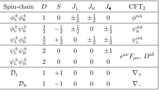
Spin-chain D S JL JR J• CFT2φ±Lφ
±
R 1 0 ±12 ±12 0 φαα˙
φ±Lψ
±
R 32 −12 ±12 0 ±12 ψRα˙a˙
ψL±φ
±
R 32 +12 0 ±21 ±12 ψLαa˙
ψ±Lψ
±
R 2 0 0 0 ±1
ǫµνFµν,Da˙b˙ ψ±Lψ
∓
R 2 0 0 0 0
DL 1 +1 0 0 0 ∇+
[image:13.595.168.429.83.231.2]DR 1 −1 0 0 0 ∇−
Table 1. Charges of the states in the representation (−1 2;
1
2)L⊗(− 1 2;
1
2)R and their relation to
the degrees of freedom of the spin-chain and CFT2. We useφ
±
L/R to denote the su(2)L/R doublet
of scalars in the (−1 2;
1
2)L/R representation, whileψ
±
L/R denotes the two fermions. The su(1,1)L/R
descendants are obtained by acting on these states withDL/R.
The states appearing in the representation9(−1
2;12)L⊗(−12;12)Rof this algebra were used to
construct the all-loop massive S matrix of the AdS3×S3×T4 superstring [18]. We collect them in table 1. To compare these states with the ones appearing in the field theory, we identify thesu(2)L⊕su(2)R⊂psu(1,1|2)L⊕psu(1,1|2)Rwith theso(4) we got by reducing
from six to two dimensions. We further let D measure the dimension and S the Lorentz spin. Finally we identifyJ• with theu(1) part of the su(2)• R-symmetry. We will now see how the states in the (−12;12)L⊗(−12;12)R match the field theory states.
First we have four scalars with dimension 1 transforming as a bispinor under su(2)L⊕
su(2)R. These correspond to the fields φαα˙. There are eight dimension 32 fermions that
have charge±12 underJ•. The fermions with spin +12 are doublets undersu(2)Rand those
with spin −12 are doublets under su(2)L. This matches the chiral and anti-chiral spinors
ψαLa˙ and ψ
˙
αa˙
R . Thesu(1,1)L andsu(1,1)R descendants are obtained by acting withDL and
DR. These correspond to the left- and right-moving covariant derivatives ∇t± ∇x.
Finally, there are four bosons of dimension 2, which are only charged under su(2)•, which decompose into a singlet and a triplet. The triplet can be identified with the auxiliary field Da˙b˙, while the singlet comes from the field strengthǫµνFµν = 2ǫµν∇µAν. Hence, the field strength multiplet perfectly fits into (−12;12)L⊗(−12;12)R.
The multiplet discussed here is very similar to the field strength multiplet of N = 4 SYM (see e.g. ref. [38]). However, the two-dimensional field strength has only a single component Ftx =−Fxt. Further, as seen above the field strength multiplet contains the normally auxiliary field Da˙b˙ which now is dynamical. In table 1 we also summarise the identifications of the spin-chain and CFT2 variables.
The states in the adjoint hypermultiplet can also be organised into psu(1,1|2)L ⊕
psu(1,1|2)R representations. However, in this case the representations are reducible. The
9We denote by (−1 2;
1
2) the short representation of psu(1,1|2) having highest weights− 1 2 and
1 2 for its
bosonic sub-algebrassu(1,1) andsu(2), respectively. The representation (−1 2;
1 2)
∗ differs from (−1 2;
1 2) by
JHEP06(2015)103
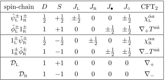
spin-chain D S JL JR J• J◦ CFT2˜ ψL±1
±
R 12 +12 ±12 0 0 ±12 χαaL˙
˜ φ±L1
±
R 1 +1 0 0 ±12 ±12 ∇+Taa˙
1±Lψ˜
±
R 12 −12 0 ±12 0 ±12 χαaR
1±Rφ˜
±
R 1 −1 0 0 ±21 ±12 ∇−Taa˙
DL 1 +1 0 0 0 0 ∇+
[image:14.595.166.431.83.212.2]DR 1 −1 0 0 0 0 ∇−
Table 2. Charges of the states in the representation 1±
L ⊗(− 1 2;
1 2)
∗
R and (− 1 2;
1 2)
∗
L⊗1
±
R and their
relation to the degrees of freedom of the spin-chain and CFT2. The fermions ˜ψ
±
L/Rform ansu(2)L/R
doublet and ˜φ±
L/Rdenote the two bosons in the (− 1 2;
1 2)
∗
L/R representations. Thesu(1,1)L/R
descen-dants are again obtained by acting withDL/R.
scalarsT±± have vanishing dimensions, spin andsu(2)
L⊕su(2)Rcharge. Hence, they form
singlets under psu(1,1|2)L⊕psu(1,1|2)R. However, they have spin 1/2 under both su(2)• and su(2)◦.
The remaining states of the hypermultiplet are charged under either psu(1,1|2)L or
psu(1,1|2)R. The left-moving fermionsχ+L± are the highest-weight states of (−12;12)∗L⊗1
±
R,
where 1±R denotes two psu(1,1|2)R singlets that form a doublet under su(2)◦. The other states in these representations are given by χ−±L and ∇+T±± as well as the su(1,1)L
descendants obtained by acting with ∇+. Similarly, the right-moving fermions χ+R± are
highest-weight states of the modules 1±L⊗(−12;12)∗R, which further containχ
−±
R and∇−T±±
as well as the states obtained by the action of ∇−. The charges of the states in these multiplets and the identification of spin-chain and CFT2 degrees of freedom are summarised in table2. This structure matches the reducible spin chain constructed in ref. [22].
4.3 Spin-chain states
We can now construct local operators using the states in the field strength multiplet and adjoint hypermultiplet. The simplest such state is the 1/2-BPS ground state
tr
(φ++)L
. (4.7)
Starting with this state we can obtain excited states by replacing the field at a site by any other adjoint field. Let us first restrict ourselves to the fields in the field strength multiplet. Such an operator will consist ofLsites each containing a state from the (−1
2;12)L⊗(−12;12)R
representation of psu(1,1|2)L⊕psu(1,1|2)R. This is exactly the operators that appear in
the integrable spin-chain constructed in [18]. The Hamiltonian acting on the spin-chain is given by the chargeH=D−J. In the next section we will calculate the one-loop correction to this Hamiltonian in a closed sub-sector.
The ground state (4.7) is the highest weight state in the short (−L
2;L2)L⊗(−L2;L2)R
representation ofpsu(1,1|2)L⊕psu(1,1|2)R, and carriesu(1) chargesD−J = 0 andM = 0.
JHEP06(2015)103
by the fields in the field strength multiplet can be grouped into two sets. Replacing one ofthe fieldsφ++ in the ground state by any of the fields
φ−+, ∇+φ−+, ψ++L , ψ
−+
L (4.8)
results in a state withD−J = 1 and M = +1. We can also consider the excitations
φ+−, ∇−φ+−, ψ++R , ψ
−+
R (4.9)
which carry charges D−J = 1 and M = −1. These two sets of excitations form two multiplets of the centrally extendedpsu(1|1)4c.e.used to construct the S matrix in [21]. The remaining fields in the field strength multiplet can be though of as composite excitations constructed out of the eight fundamental excitations.
Let us now consider excitations created from fields in the adjoint hypermultiplet. The four bosonic and four fermionic fields
T±±, χ+L±, χ
+±
R , (4.10)
all carry charges D−J = 0 and M = 0. They can be inserted into the operator with no cost of energy, and hence correspond to gapless excitations. Since the scalars Taa˙ form singlets under psu(1,1|2)L⊕psu(1,1|2)R the resulting spin-chain states are exactly
of the type that appears in the reducible spin-chain discussed in [22]. The excitations fit perfectly in the massless psu(1|1)4c.e.⊕su(2)◦ representation discussed in [11, 12]. While the operators containing these fields form reducible short representations at tree-level, we expect them to join into long irreducible representations once we include the interactions. A similar mechanism explains the fact that at zero coupling this theory seems to have too many chiral primaries with respect to the supergravity dual or to the symmetric product orbifold CFT [39]. Naively, arbitrary products of χ+L±, χ
+±
R give chiral primary composite
operators. However, all but few of these are accidental chiral primaries, whose dimension is corrected at non-zero coupling [22]. We hope return to the investigation of the exact details of these mechanisms and of the chiral ring in the future.
5 One-loop dilatation operator in the so(4) sector
In this section we will compute, in the planar limit, the one-loop anomalous dimensions of operators in the effective CFT2 proposed by Witten. We restrict ourselves to operators made up of scalar fields from the vector multiplet, which form a one-loop closed subsector charged under so(4).10 We find that the computation of these anomalous dimensions can
be re-phrased in terms of finding the spectrum of a nearest-neighbour Hamiltonian for a homogenous so(4) spin chain, in a manner similar to the seminal work of Minahan and Zarembo [23]. As we will show explicitly, such an Hamiltonian has precisely the right form to beintegrable.
Witten’s prescription for the dynamics for states localised near the origin of the Higgs branch is closely related to the “large-N” approach11 widely used in the study of sigma
JHEP06(2015)103
models [41]. In the present setting it is Nf that plays the role of “large-N”, while takingNc large will ensure that we can restrict to single-trace operators. Let us then consider single-trace operators made out of scalar fields from the vector multiplet,
OA= tr φα1α˙1φα2α˙2· · ·φαJα˙J. (5.1)
Since these operators are charged only under so(4) = su(2)L ⊕su(2)R we refer to it as
the so(4) sector. Our goal is to find the one-loop dilatation operator acting on these operators. To extract the dilatation operator we consider the one-loop corrections to the local operators. These corrections are generally UV divergent, which means we need to introduce counter-terms and renormalised operators
OI,ren=ZIJOJ,bare, Z = 1 +λ2Z2+· · ·. (5.2)
The matrix Z cancels the UV divergences in the one-loop corrections, and introduces a mixing between different operators. In a perturbative calculation it can be extracted as minus the divergent piece of the sum of all Feynman diagrams. In dimensional regulari-sation we consider the theory in D= d+ 2ǫ dimensions and divergences appear as poles in ǫ. For non-zero ǫ the coupling constant is dimensionful. Hence we introduce as mass parameterµ so that the full coupling constant can be written asµ2ǫλ. The corrections to the dilatation operator can then be extracted as
δD= µ d
dµlogZ(µ
2ǫλ, ǫ)
ǫ=0
. (5.3)
In the planar limit, the one-loop dilatation operator acts locally on two neighbouring fields of the operators. From so(4) symmetry we expect it to take the form
L X
k=1 (δb1
a1δ
˙
b1
˙
a1)· · ·(δ
bk−1
ak−1δ
˙
bk−1
˙
ak−1)M
bkb˙kbk+1b˙k+1
aka˙kak+1a˙k+1(δ
bk+2
ak+2δ
˙
bk+2
˙
ak+2)· · ·(δ
bJ aJδ
˙
bJ
˙
aJ), (5.4)
where M is an so(4) invariant tensor, which can be built out of the identity 1, the per-mutation Pand the trace K. The dilatation operator should preserve supersymmetry. In particular it should annihilate chiral primary operators such as (4.7), since the dimension of these operators is protected. Since this operator is symmetric and traceless, we can impose supersymmetry by requiring the tensorM to take the form
M =c1(1−P) +c2K, (5.5)
for some constantsc1 and c2. Hence, we only need to consider Feynman diagrams that act non-trivially in flavour space.
5.1 “One-loop” Feynman diagrams
JHEP06(2015)103
conformal invariance, cf. equation (3.5), and the effective interaction vertices are given byone-loop diagrams of LIR, like in (3.8). This provides a systematic expansion of Leff in Feynman diagrams.
We are interested in the limit of a large number of colours Nc and flavours Nf, with the ’t Hooft couplingλ=Nc/Nf fixed and small. The (effective) diagrams that contribute to the two-point function at one loop and are divergent by power counting are
, (5.6)
where the straight and wiggly double lines indicate the effective propagators of the scalars and gluons from the vector multiplet, and the fat dots represent effective vertices obtained by one-loop sub-diagrams with a field from the fundamental hypermultiplet running in the loop. The large blob in the last diagram represents the one-loop self energy. As we saw in eq. (3.8), the four-scalar interaction comes from the diagrams
= + , (5.7)
while the gluon-scalar interaction is given by
= + . (5.8)
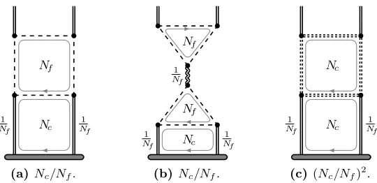
Above, the single dashed and solid lines correspond to fundamental fermions and scalars, respectively. We refer to the diagrams in (5.6) as one-loop diagrams, because they all give a contribution proportional to the coupling λ = Nc/Nf. In practice, to compute them we need to plug in the effective vertices (5.7), (5.8), yielding several loops for each diagram. Let us see in more detail how this counting of λgoes for the diagrams in (5.6). We first note that the above vertices all contain a single loop of fields from the fundamental hypermultiplet, which gives an overall factor of Nf. Furthermore, the effective action for the fields in the vector multiplet is proportional toNf. Hence, each double line propagator in (5.6) gives a factor 1/Nf. Finally, in each diagram there is a single sum over colour indices in the loop, which gives a factor of Nc. Since the number of effective vertices in each diagram is one less than the number of internal propagators the overall factor for each diagram isNc/Nf.
In principle we should also consider the diagrams above, but with the fields from the fundamental hypermultiplet replaced by the corresponding fields in the adjoint hypermul-tiplet. However, in that case the sums over flavours in the loops are replaced by a sum over colours. Hence, the resulting diagrams are suppressed at smallλ. The counting of factors of Nc and Nf is illustrated in figure1.
JHEP06(2015)103
1
Nf
1
Nf
Nc
Nf
(a) Nc/Nf.
1
Nf
1
Nf
1
Nf
Nc
Nf
Nf
(b)Nc/Nf.
1
Nf
1
Nf
Nc
Nc
[image:18.595.164.434.81.212.2](c) (Nc/Nf)2.
Figure 1. Example of counting of factors of Nc and Nf for three diagrams. The double lines represent adjoint fields and the single line give particles transforming in the fundamental repre-sentation of the gauge group. Each closed loop gives a factor of Nc or Nf depending on which representation the fields in the loop transform under. Additionally, each propagator for a field in the vector multiplet give a factor 1/Nf. The first two diagrams are proportional to Nc/Nf and hence count as one-loop diagrams. The dotted propagator in the third diagram corresponds to a fermion in the adjoint hypermultiplet. This diagram is proportional to (Nc/Nf)2 and is therefore suppressed in the weakly-coupled planar limit.
supersymmetry. Hence, we do not need to calculate those diagrams. The third diagram in (5.6) gives an so(4) trace in flavour space. By expanding the effective vertices in this diagram in terms of the one-loop diagrams with a fundamental hyper, we find four different diagrams. However, all four vanish due to symmetry as detailed in appendixC. Hence, the first diagram in (5.6) is the only one we have to compute.
5.2 Computation of one-loop dilatation operator
In this sub-section we consider the first diagram in (5.6). As was shown above, it is only this diagram that has a potentially non-trivialso(4) flavour structure and hence is needed to determine the dilatation operator. We may expand the diagram by plugging in the effective vertices (5.7) and (5.8)
= + + . (5.9)
In fact, the first of these diagram again has a trivial flavour structure and so we do not need to calculate it. The second diagram gives an so(4) trace in flavour space, and we compute it in appendixC. There we show that the corresponding integral is UV-finite, and therefore does not contribute to the mixing matrix. We are only left with the last diagram, the fermion box
. (5.10)
The left- and right-moving fermions λL and λR in the hypermultiplet are charged under
JHEP06(2015)103
¯
λL
φ λR
¯
λR
φ λL
¯
λR φ
λL ¯ λL φ λR =
ak a˙k ak+1 a˙k+1
bk b˙k bk+1 b˙k+1
(a) δbk akδ
bk+1
ak+1ǫa˙ka˙k+1ǫ
˙
bkb˙k+1.
¯
λR
φ λL
¯
λL
φ λR
¯
λL φ
λR ¯ λR φ λL =
ak a˙k ak+1 a˙k+1
bk b˙k bk+1 b˙k+1
(b)ǫakak+1ǫbkbk+1δ
˙
bk
˙
akδ
˙
bk+1
˙
[image:19.595.121.472.87.209.2]ak+1.
Figure 2. The flavour structure of the fermion box diagram for the two fermion chiralities. The dashed red lines represent the su(2)L flavour, while thesu(2)R flavour is represented by solid blue
lines. A vertical line connecting the operator at the bottom with an external line corresponds to a Kroneckerδwhile a line connecting two sites of the operator or two external lines corresponds to a Levi-Civita tensorǫ.
each couple φ to λL and λR. Hence, the diagram in (5.10) in fact corresponds to two
diagrams that differ in the assignment of chiralities of the fermions in the loop. It turns out that the two diagrams result in two different flavour structures.
Let us consider such flavour structures in more detail. In each propagator and each vertex the su(2)L and su(2)R indices are contracted by invariant ǫ-symbols as shown in
figure 2. In the figure the su(2)L (su(2)R) indices are represented by dashed red (solid
blue) lines. A line connecting the operator at the bottom with an external line gives a contraction with a Kronecker δ while a line connecting two sites of the operator or two external lines contracts the indices with a Levi-Civita tensor ǫ.
The computation of the divergence for each of these diagrams is somewhat involved due to the propagator (3.5). It is straightforward, however, to show that the difference of the two resulting integrals is finite, see appendixC. To perform the calculation for thesum
of the diagrams we work in two steps. We first compute the integral in dimension dusing the propagator of (3.5), that in momentum space is
hφαα˙(−p)φββ˙(+p)i= C ′ǫαβǫα˙β˙
|p|2(d/2−1). (5.11) The resulting integral has a UV log-divergence in any d > 2. We then check that the diagram remains UV divergent also when takingd→2. As the diagram (5.10) is logarith-mically divergent in the UV it contributes to the dilatation operator. We again relegate the details of such calculation to appendixC.
We have concluded that the divergent part of the fermion-box diagram yields a con-tribution to the mixing matrix M of the form
Mbkb˙kbk+1b˙k+1
aka˙kak+1a˙k+1 ∝δ
bk akδ
bk+1
ak+1ǫ
˙
bkb˙k+1ǫ
˙
aka˙k+1+ǫ
bkbk+1ǫ
akak+1δ
˙
bk
˙
akδ
˙
ak+1
˙
ak+1. (5.12)
To simplify this we introduce the identity operator 1 and permutation P acting on the tensor product of two spin-1/2su(2) representations. If Ψa is ansu(2) doublet this action can be written as
JHEP06(2015)103
The combination 12(1−P) then represents a projector onto thesu(2) singlet1
2(1−P) |Ψ
aΨbi= 1 2(|Ψ
aΨbi − |ΨbΨai) = 1 2ǫ
abǫ
cd|ΨcΨdi . (5.14)
Since the divergence of both fermion box diagrams shown in figure2is the same, the flavour structure of the mixing matrixM can then be written as
M ∝1⊗(1−P) + (1−P)⊗1 = 1⊗1−P ⊗P+ (1−P)⊗(1−P)
=1−P+K. (5.15)
Since the above operator annihilates the supersymmetric vacuum (4.7) by itself, and since the diagrams that we have refrained from computing so far do not, we find that these must cancel by supersymmetry.
We conclude that the one-loop dilatation operator in this sector is given by
δD∝ Nc Nf
L X
k=1
1−P+Kk,k+1, (5.16)
in theso(4) sector, up to an overall numerical constant. This is precisely the Hamiltonian of the integrable so(4) spin-chain [42,43].
6 Conclusions
In this paper we have investigated the Higgs-branch CFT2 states that are localised near the small-instanton singularity. Using Witten’s description of such states [32], we showed that they can be analysed in a planar, weak-coupling limit, with λ≡Nc/Nf playing the role of the ’t Hooft coupling and non-planar diagrams suppressed by powers of 1/N2
c. We demonstrated that at small λ and large Nc computing the anomalous dimension of such operators reduces to the calculation of the spectrum of a nearest-neighbour spin chain. Further, in a sub-sector of the theory, we showed that the Hamiltonian of the spin-chain is integrable.
JHEP06(2015)103
in an integrable Hamiltonian for the vector representation of so(4) in a manner that isreminiscent of [23]. This is the first appearance of integrability on the CFT2 side of the duality. Together with the evidence for integrability that has been found on the string theory side [11–14], it provides a powerful argument for a holographic integrability descrip-tion of AdS3/CFT2. This evidence leads us to suggest that the perturbative closed strings of the R-R AdS3 background are dual to CFT2 states localised near the small-instanton singularity.
In a forthcoming paper, we will return to the computation of the complete CFT2 spin-chain Hamiltonian. There, we will also address the issue of length-changing effects that are expected to occur in the complete spin-chain, much as they do in N = 4 SYM [44]. This should allow us to understand better, from the weakly-coupled CFT2 point of view, how the massless modes enter into the reducible spin-chain description introduced in [22]. It will also allow for a CFT2-based understanding of the S matrix constructed in [11,12]. In this context it will be particularly illuminating to extend the analysis of the chiral-ring of the CFT2 that was initiated in [22].
It is widely believed that the SymN(T4) orbifold can be found at some point in the moduli space of the N = (4,4) CFT2 that we have been investigating in this paper. However, it appears to be much harder to understand the spin-chain picture starting from the SymN(T4) orbifold point [45], though many suggestive connections seem to exist. It would be interesting to see whether it is possible to deform the spin-chain [18, 22] to approach the SymN(T4) orbifold point. It is not clear to us whether the connection to the orbifold can be fully understood in the small λlimit.12
Throughout this paper we have focused on the CFT2 description of the D1-D5 system, or in other words on string geometries supported by R-R three-form flux only. More generally, the AdS3/CFT2 correspondence is believed to hold for configurations involving NS5-branes and fundamental strings in addition to the D1- and D5-branes. In this case the string geometry is supported by a mixture of NS-NS and R-R three-form flux, giving a family of backgrounds related by Type IIB S-duality. The all-loop worldsheet S matrix for these backgrounds is known [13,46], and we expect also these dualities to be governed by a quantum integrable system. It would be interesting to understand whether an integrable spin-chain picture emerges in this setting too. It would also be interesting to understand how recent work on higher-spin limits of AdS3/CFT2, such as [47], can be related to our findings. Recent progress on understanding the large N = (4,4) AdS3/CFT2 duality [48] opens up the possibility of establishing the expected connections to integrability more firmly.
The “large-N” method (which here means largeNf) is particularly useful in the study of the effective theory describing states localised near the origin of the Higgs branch, as was originally advocated by Witten [32]. In this paper, we have used this approach to perform some simple computations of anomalous dimensions at leading order. But large-N techniques have been very widely exploited for a long time and an extensive set of tools exists to perform calculations in this approach. As a result, we expect that these
JHEP06(2015)103
methods, combined with integrability, will lead to significant advances in understandinggeneric unprotected quantities in the AdS3/CFT2 correspondence in the near future.
Acknowledgments
We would like to thank Gleb Arutyunov, Riccardo Borsato, Stefano Cremonesi, Nick Dorey, Sergey Frolov, Amihay Hanany, Chris Hull, Juan Maldacena, Joe Minahan, Sameer Murthy, Leonardo Rastelli, David Tong, Alessandro Torrielli, Arkady Tseytlin and Kostya Zarembo for helpful discussions. We are particularly grateful to Riccardo Borsato, Tom Lloyd and Alessandro Torrielli for collaborating with us on a number of related projects. O.O.S.’s work was supported by the ERC Advanced grant No. 290456, “Gauge theory — string theory duality”. A.S.’s work is funded by the People Programme (Marie Curie Actions) of the European Union, Grant Agreement No. 317089 (GATIS). A.S. also acknowledges the hospitality at APCTP where part of this work was done, as well as hospitality by ´Ecole Normale Sup´erieure in Paris and interesting discussions with Benjamin Basso, Volodya Kazakov and Jan Troost. B.S. acknowledges funding support from an STFC Consolidated Grant “Theoretical Physics at City University” ST/J00037X/1.
A Gamma matrices
We use the gamma matrices
Γ0 = +iσ2⊗σ3⊗σ3,
Γ1 =−σ1⊗ 1 ⊗σ3,
Γ2 =−σ2⊗σ2⊗ 1,
Γ3 = +σ2⊗σ1⊗σ3, Γ4 =−σ1⊗σ2⊗σ1,
Γ5 = +σ1⊗σ2⊗σ2.
(A.1)
In this basis a generic six-dimensional spinor can be written as a tri-spinor Ψα0α1α2.
In-troducing the intertwiners
C=−Γ0, B = Γ0125, T =BtC. (A.2)
the Gamma matrices satisfy
CΓµC−1=−(Γm)†, BΓµB−1=−(Γm)∗, TΓµT−1 = +(Γm)t. (A.3)
We also have
JHEP06(2015)103
It is also useful to noteCΓ0= 1 ⊗ 14,
CΓ1=σ3⊗γˆ2345,
CΓ2= 1 ⊗γˆ2,
CΓ3= 1 ⊗γˆ3,
CΓ4=σ3⊗γˆ4,
CΓ5=σ3⊗γˆ5,
(A.5)
where we have introduced theso(4) gamma matrices
(ˆγi)aa,b˙ b˙=
0 (γi) ab˙ (˜γi)ab˙ 0
!
, (A.6)
with
γ2 = +σ3, γ3 =−i1, γ4 = +σ2, γ5 = +σ1, γ˜i = +(γi)†, (A.7)
and
ˆ
γ2345=σ3⊗1. (A.8)
We also have
TΓ0= +1 ⊗t,
TΓ1= +1 ⊗tγˆ2345,
TΓ2= +1 ⊗tγˆ2,
TΓ3= +1 ⊗tγˆ3,
TΓ4= +σ3⊗tˆγ3,
TΓ5= +σ3⊗tˆγ5,
(A.9)
where the four-dimensional transpose intertwiner is given by
t=σ3⊗ǫ. (A.10)
B G-functions
It is useful to introduce the basic one-loop integrals
Z dDk (2π)D
1
k2α(k−p)2β =
1
p2(α+β−D/2)G(α, β),
Z dDk (2π)D
kµ
k2α(k−p)2β =
pµ
p2(α+β−D/2)G1(α, β),
Z dDk (2π)D
k·(p−k) k2α(k−p)2β =
1
p2(α+β−1−D/2)G2(α, β).
(B.1)
The function Gis given by
G(α, β) = 1 (4π)D/2
Γ(α+β−D/2)Γ(D/2−α)Γ(D/2−β)
JHEP06(2015)103
The integrals with non-trivial numerators can be expressed in terms of the above integral asG1(α, β) = 1
2 G(α, β)−G(α, β−1) +G(α−1, β)
,
G2(α, β) = 1
2 G(α, β)−G(α, β−1)−G(α−1, β)
.
(B.3)
C Regularisation of Feynman diagrams
In this appendix we present the details of the Feynman diagram calculation discussed in section 5. Since we are in two dimensions the IR properties of the theory are rather delicate [32]. What is more, the effective propagator for the vector multiplet fields that follows from the two-point function (3.5) is logarithmic in momentum space. All this makes it difficult to evaluate the loop-momenta integrals. To overcome such technical complications we propose the following method. We will compute the one-loop anomalous dimensions in a largeNf expansion for a general dimension d >2, following which we will take the limit d → 2.13 This method is useful because the effective propagator for the
scalarsφ in dimension d >2 has a simple form in momentum space (5.11). It also allows us to retain much better control over the IR region of momentum integration. We believe this prescription is physically well motivated, because we are interested in the anomalous dimensions of the CFT2 which are related to the UV properties of the theory. Furthermore, within the large-N approach anomalous dimensions are often computed in a similar manner for generic d[49,50] and, when finite, thed→2 limit can be taken.
The leading order diagrams that we are interested in are given in equation (5.6). The diagrams that give non-trivial flavour interactions are
, (C.1)
and
. (C.2)
The four diagrams in (C.1) involving a gluon exchange all vanish by symmetry. As an exam-ple of this let us consider the lower subgraph of the second and fourth diagram containing a scalar bubble
. (C.3)
13The loop-momentum integrals will be performed in dimensional regularisation — we will evaluate them
JHEP06(2015)103
This integral can be represented by the two diagramsµ µ
p +
µ µ
p
, (C.4)
where the arrows indicate a factor of the corresponding momentum in the numerator of the integral. Reflecting the second diagram horizontally gives the first diagram but with the momentum insertion in the opposite direction so that the two diagrams sum to zero. A similar argument can be used to show that the fermion triangle appearing in the bottom of the third and fifth diagram of (C.1) vanishes.
The remaining leftmost integral in (C.1) is given by a product of two bubble integrals. One bubble consists of scalar fields from the vector multiplet and one of scalars from the hypermultiplet, Ibb = BhypBvec. Let us consider the bubble from the hypermultiplet. Power counting dictates that such an integral must be UV-convergent in anyd <4, and in particular in d= 2 where we want to compute it. Dimensional regularisation yields
Bhyp = Z
dDk (2π)D
1
k2(k−p)2 = 1
p2(2−D/2)G(1,1)≈ 1 πp2
1
ǫ, (C.5)
where in the last step we expanded around D= 2 +ǫ, and the function Gwas introduced in appendix B. Clearly this pole is due to an infrared divergence, and as such will not contribute to the mixing matrix. The bubble of scalars from the vector multiplet on the other hand appears, by power-counting, to be polynomially UV divergent (but IR-finite). In dimensional regularisation we have
Bvec= Z
dDk (2π)D
1
k2(d/2−1)(k−p)2(d/2−1) =
1
p2(d−2−D/2)G
d 2 −1,
d 2−1
. (C.6)
We want to see whether this expression is UV divergent in dimensiond, i.e., we setD=d+ǫ. We obtain, up to numerical prefactors
Bvec=p2(2−d/2) 1
(d/2−2)2Γ[d/2−2]+O(ǫ). (C.7)
Not only is this expression regular atd= 2, but in fact itvanishes, and it does so regardless of how we send D → d→ 2.14 Clearly the bubbles are well-behaved in the UV, and Ibb cannot contribute to the mixing matrix.
We are left with the fermion box diagram (C.2). This diagrams gives rise to two integralsI1 and I2 which differ in the chiralities of the fermions. Diagrammatically these
14Interestingly, it vanishes even in d = 0, where we would expect the d = 2 quadratic divergence to
JHEP06(2015)103
integrals can be represented byI1 =
d/2 −
1 d/2−
1 +
−
+
−
p1 p2
p1+p2
I2 =
d/2 −
1 d/2−
1
−
+
−
+
p1 p2
p1+p2
. (C.8)
The arrows on the propagators in the boxes represent a factor of momentum in the numer-ator, with the ±next to the arrow indicating the component. The label below the double lines at the bottom serve as a reminder of the non-canonical weight of the propagator of the scalar in the vector multiplet. To evaluate the UV divergence of these integrals while avoiding IR divergences we can set the external momenta top1=−p2 =p.
We will start by showing that the two integralsI1andI2 have the same UV divergence. Let us therefore consider the difference between these integrals
I1−I2 = + + −
−
d−2
− − −
+
+
d−2
. (C.9)
Since we have set p1+p2= 0, the two scalar propagators at the bottom have merged into a single propagator of weightd−2. We can now perform the bubble integrals to obtain
I1−I2 =G1(1, d−2)
−
d−D2 + 1 −+
+ −
+
d−D2 + 1
+−
−
. (C.10)
The remaining loop integrals are tensor valued and anti-symmetrised. Since the only available tensors are the metric and the external momentum p, the difference of the two integrals vanishes and the UV divergences ofI1 and I2 coincide.15
Since the integrals I1 and I2 have the same UV divergence we can consider their sum, which can be interpreted as a single fermion box diagram with a Dirac fermion running in the loop. This leads to an integral of the form
I1+I2= Z
dDk dDq (2π)2D
tr /k(/k−/p
1)(k/+/p2)(k/−/q)
k2(k−p
1)2(k+p2)2(k−q)2(q−p1)2(d/2−1)(q+p2)2(d/2−1)
. (C.11)
Again the UV divergence can be evaluated by setting p1 = −p2 = p. The trace in the numerator gives rise to three different contractions, which diagrammatically can be
repre-15Note that the full integralsI
1andI2are not necessarily identical. However, because the UV divergence
JHEP06(2015)103
sented asI1+I2 = 4 µ ν µ ν
d−2
+ ν µ
µ
ν
d−2
− ν ν
µ
µ
d−2
. (C.12)
In the above diagrams the arrows again indicate factors of momenta in the numerator, and the indicesµandν indicate which momenta are to be contracted. Performing the one-loop bubble integral we are left with three identical terms which add up to
I1+I2= 4G1(1, d−2)
µ
d−D2 µ
= 4G1(1, d−2)
Z dDk
(2π)D
k·(p−k) k2(k−p)2(d−D/2).
(C.13)
If we go ahead and perform the remaining integration by dimensional regularisation we find
I1+I2 =− 4
p2(d−D)G1(1, d−2)G2(1, d−D/2) (C.14)
which has a simple pole at d=D for any d >2. However, taking the limit d→2 in this expression is subtle. Instead, we re-express the integral using Feynman parameters as
I1+I2 =−4G1(1, d−2)
Z dDk
(2π)D 1
k2(d−D2)
+ 4
d−D 2
G1(1, d−2) Z
dDk (2π)D
Z 1
0
dx x d−D
2−1(p·k+xp2)
(k2+x(1−x)p2)d−D
2+1
.
(C.15)
The integral in the second line is UV convergent. Performing the integral in the first line we get
I1+I2 ≈ − 8G1(1, d−2) (4π)D/2Γ(D/2)
Z Λ
µ
dk
k2(d−D)+1 =−
4G1(1, d−2) (4π)D/2Γ(D/2)
Λ2(D−d)−µ2(D−d)
D−d , (C.16)
where we have dropped terms that are not UV divergent and Λ andµ are cutoffs at large and small momentum. Using the definition ofG1 we get
I1+I2 ≈ 4π (4π)D
csc((d−D/2)π) Γ(d−2)Γ(D−d+ 2)
Λ2(D−d)−µ2(D−d)
d−D . (C.17)
In the above calculation the dimension d has been introduced in the propagator to avoid IR divergences, whileD has been introduced in the integrations to avoid UV divergences. Hence we now need to take the limit wheredand Dapproach 2 with
JHEP06(2015)103
A natural way to do this is to first sendD→d, and then d→2, which results inI1+I2 ≈ 8π (4π)d
csc(dπ/2) Γ(d−2) log
Λ µ ≈ −
1 π2 log
Λ
µ, (C.19)
so that the fermionic box diagram (C.2) is UV divergent. This expression also appears IR divergent when we send µ to zero. However, in the full fermion box integral with the momentum assignment we have made there is no such divergence, so this IR divergence is cancelled by a contribution from the UV convergent integral in (C.15) that we have dropped.
Open Access. This article is distributed under the terms of the Creative Commons Attribution License (CC-BY 4.0), which permits any use, distribution and reproduction in any medium, provided the original author(s) and source are credited.
References
[1] J.M. Maldacena,The Large-N limit of superconformal field theories and supergravity,
Int. J. Theor. Phys.38 (1999) 1113[Adv. Theor. Math. Phys. 2(1998) 231] [hep-th/9711200] [INSPIRE].
[2] E. Witten,Anti-de Sitter space and holography,Adv. Theor. Math. Phys. 2(1998) 253 [hep-th/9802150] [INSPIRE].
[3] S.S. Gubser, I.R. Klebanov and A.M. Polyakov,Gauge theory correlators from noncritical string theory,Phys. Lett.B 428(1998) 105[hep-th/9802109] [INSPIRE].
[4] G. Arutyunov and S. Frolov,Foundations of the AdS5×S5 Superstring. Part I,
J. Phys.A 42(2009) 254003[arXiv:0901.4937] [INSPIRE].
[5] N. Beisert et al.,Review of AdS/CFT Integrability: An Overview,
Lett. Math. Phys.99(2012) 3[arXiv:1012.3982] [INSPIRE].
[6] A. Babichenko, B. Stefa´nski Jr. and K. Zarembo,Integrability and theAdS3/CF T2
correspondence,JHEP 03(2010) 058[arXiv:0912.1723] [INSPIRE].
[7] P. Sundin and L. Wulff,Classical integrability and quantum aspects of the
AdS3×S 3
×S3×S1 superstring,JHEP 10 (2012) 109[arXiv:1207.5531] [INSPIRE]. [8] A. Cagnazzo and K. Zarembo,B-field inAdS3/CF T2 Correspondence and Integrability,
JHEP 11 (2012) 133[arXiv:1209.4049] [INSPIRE].
[9] J.R. David, G. Mandal and S.R. Wadia,Microscopic formulation of black holes in string theory,Phys. Rept.369(2002) 549[hep-th/0203048] [INSPIRE].
[10] A. Sfondrini, Towards integrability forAdS3/CF T2,J. Phys.A 48(2015) 023001
[arXiv:1406.2971] [INSPIRE].
[11] R. Borsato, O. Ohlsson Sax, A. Sfondrini and B. Stefa´nski Jr.,Towards the All-Loop Worldsheet S Matrix forAdS3×S
3
×T4
, Phys. Rev. Lett.113(2014) 131601 [arXiv:1403.4543] [INSPIRE].
[12] R. Borsato, O. Ohlsson Sax, A. Sfondrini and B. Stefa´nski Jr.,The completeAdS3×S3×T4