INERTIAL GAME DYNAMICS AND
APPLICATIONS TO CONSTRAINED OPTIMIZATION
∗RIDA LARAKI† AND PANAYOTIS MERTIKOPOULOS‡
Abstract. Aiming to provide a new class of game dynamics with good long-term convergence properties, we derive a second-order inertial system that builds on the widely studied “heavy ball with friction” optimization method. By exploiting a well-known link between the replicator dynamics and the Shahshahani geometry on the space of mixed strategies, the dynamics are stated in a Riemannian geometric framework where trajectories are accelerated by the players’ unilateral payoff gradients and they slow down near Nash equilibria. Surprisingly (and in stark contrast to another second-order variant of the replicator dynamics), the inertial replicator dynamics are not well-posed; on the other hand, it is possible to obtain a well-posed system by endowing the mixed strategy space with a different Hessian–Riemannian (HR) metric structure, and we characterize those HR geometries that do so. In the single-agent version of the dynamics (corresponding to constrained optimization over simplex-like objects), we show that regular maximum points of smooth functions attract all nearby solution orbits with low initial speed. More generally, we establish an inertial variant of the so-called folk theorem of evolutionary game theory, and we show that strict equilibria are attracting in asymmetric (multipopulation) games, provided, of course, that the dynamics are well-posed. A similar asymptotic stability result is obtained for evolutionarily stable states in symmetric (single-population) games.
Key words. game dynamics, folk theorem, Hessian–Riemannian metrics, learning, replicator dynamics, second-order dynamics, stability of equilibria, well-posedness
AMS subject classifications.34A12, 34A26, 34D05, 70F20, 70F40, 90C51, 91A26
DOI.10.1137/130920253
1. Introduction.
One of the most widely studied dynamics for learning and
evolution in games is the classical replicator equation of Taylor and Jonker [47], first
introduced as a model of population evolution under natural selection. Stated in the
context of finite
N
-player games with each player
k
∈ {
1
, . . . , N
}
choosing an action
from a finite set
A
k, these dynamics take the form
(RD)
x
˙
kα=
x
kαv
kα(
x
)
−
β∈Akx
kβv
kβ(
x
)
,
where
x
k= (
x
kα)
α∈Akdenotes the mixed strategy of player
k
(i.e.,
x
kαrepresents the
probability with which player
k
selects
α
∈ A
k), while
v
kα(
x
) denotes the expected
∗Received by the editors May 8, 2013; accepted for publication (in revised form) July 13, 2015; published electronically October 6, 2015. The authors gratefully acknowledge financial support from the French National Agency for Research under grants ANR-10-BLAN-0112-JEUDY, ANR-13-JS01-GAGA-0004-01, and ANR-11-IDEX-0003-02/Labex ECODEC ANR-11-LABEX-0047 (part of the program “Investissements d’Avenir”).
http://www.siam.org/journals/sicon/53-5/92025.html
†CNRS (French National Center for Scientific Research), LAMSADE–Paris-Dauphine, and
De-partment of Economics, ´Ecole Polytechnique, 91128 Paris, France ([email protected]). ‡Corresponding author. CNRS (French National Center for Scientific Research), LIG, and Uni-versity of Grenoble Alpes, LIG, F-38000 Grenoble, France ([email protected]). This author’s research was partially supported by the Pˆole de Recherche en Math´ematiques, Sciences, et Technologies de l’Information et de la Communication under grant C-UJF-LACODS MSTIC 2012 and the European Commission in the framework of the FP7 Network of Excellence in Wireless COMmunications NEWCOM# (contract 318306).
3141
payoff to action
α
∈ A
kin the mixed strategy profile
x
= (
x
1, . . . , x
N).
1Accordingly, a considerable part of the literature has focused on the long-term
rationality properties of the replicator dynamics. First, building on early work by Akin
[2] and Nachbar [32], Samuelson and Zhang [39] showed that suboptimal, dominated
strategies become extinct along every interior trajectory of (RD). Second, the
so-called folk theorem of evolutionary game theory states that (a) Nash equilibria are
stationary in (RD); (b) limit points of interior trajectories are Nash; and (c) strict
Nash equilibria are asymptotically stable under (RD) [19,
20]. Finally, when the game
admits a potential function (in the sense of [31]), interior trajectories of (RD) converge
to the set of Nash equilibria that are local potential maximizers [19].
To a large extent, the strong convergence properties of the replicator dynamics
are owed to their dual nature as a reinforcement learning/unilateral optimization
device. The former aspect is provided by the link between (RD) and the so-called
exponential weights (EW) algorithm where players choose an action with probability
that is exponentially proportional to its cumulative payoff over time [24,
29,
37,
45,
49].
In continuous time, this process formally amounts to the dynamical system
(EW)
˙
y
kα=
v
kα,
x
kα=
exp(
y
kα)
βexp(
y
kβ)
,
and, as can be seen by a simple differentiation, (EW) is equivalent to (RD).
Dually, from an optimization perspective, the replicator dynamics can also be seen
as a unilateral gradient ascent scheme where, to maximize their individual payoffs,
players ascend the (unilateral) gradient of their payoff functions with respect to a
particular geometry on the simplex—the so-called
Shahshahani metric
, given by the
metric tensor
g
αβ(
x
) =
δ
αβ/x
αfor
x
α>
0 [42]. In this light, (RD) can be recast as
(1.1)
x
˙
k= grad
Sku
k(
x
)
,
where grad
Sku
k(
x
) denotes the unilateral Shahshahani gradient of the expected payoff
function
u
k(
x
) =
αx
kαv
kα(
x
) of player
k
[1,
17,
18,
42].
2Owing to this last
interpretation, (RD) becomes a proper Shahshahani gradient ascent scheme in the
class of potential games: the game’s potential acts as a Lyapunov function for (RD),
so interior trajectories converge to the set of Nash equilibria that are local maximizers
thereof [18,
19].
3Despite these important properties, the replicator dynamics fail to eliminate
weakly dominated strategies [38]. Thus, motivated by the success of second-order,
“heavy ball with friction” methods in optimization [3,
4,
6,
8,
16,
35], our first goal in
this paper is to examine whether it is possible to obtain better convergence properties
1In the mass-action interpretation of population games,x
kαrepresents the proportion of players
in populationkthat use strategyα∈ Ak, andvkα(x) is the associated fitness.
2For our purposes, “unilateral” here means differentiation with respect to the variables that are
directly under the player’s control (as opposed to all variables, including other players’ strategies).
3By contrast, using ordinary Euclidean gradients and projections leads to the well-known
(Eu-clidean) projection dynamics of Friedman [15]; however, because Euclidean trajectories may collide with the boundary of the game’s state space in finite time, the folk theorem of evolutionary game theory does not hold in a Euclidean context, even when the game is a potential one [41].
in a second-order setting. To that end, if we replace ˙
y
by ¨
y
in (EW), we obtain the
dynamics
(EW
2)
¨
y
kα=
v
kα,
x
kα=
exp(
y
kα)
βexp(
y
kβ)
.
These
second-order
exponential learning dynamics were studied in the very recent
paper [21], where it was shown that (EW
2) is equivalent to the
second-order replicator
equation
4(RD
2)
¨
x
kα=
x
kα⎡
⎣
v
kα(
x
)
−
β∈Akx
kβv
kβ(
x
)
⎤
⎦
+
x
kα⎡
⎣
x
˙
2kαx
2kα−
β∈Ak
˙
x
2kβx
kβ⎤
⎦
.
Importantly, under (EW
2)/(RD
2), even
weakly
dominated strategies become extinct;
such strategies may survive in perpetuity under the first-order dynamics (RD), so this
represents a marked advantage for using second-order methods in games.
That being said, the second-order system (RD
2) has no obvious ties to the gradient
ascent properties of its first-order counterpart, so it is not clear whether its trajectories
converge to Nash equilibrium in potential games. On that account, a natural way to
regain this connection would be to see whether (RD
2) can be linked to the heavy ball
with friction system
(1.2)
D
2
x
kDt
2= grad
S
k
u
k(
x
)
−
η
x
˙
k,
where
D2xkDt2
denotes the covariant acceleration of
x
kunder the Shahshahani metric
and
η
≥
0 is a friction coefficient, included in (1.2) to slow down trajectories and
enable convergence. In this way, if the game admits a potential function Φ, the total
energy
E
(
x,
x
˙
) =
12x
˙
2
−
Φ(
x
) will be Lyapunov under (1.2) (by construction), so
4From the point of view of evolutionary game theory, there is an alternative derivation of the
second-order replicator dynamics (RD2) which is based on the so-called imitation of long-term
suc-cess [21]. Focusing for simplicity on a single population, assume that each nonatomic agent in the population receives an opportunity to switch strategies at every ring of a Poisson alarm clock and ραβ denotes the correspondingswitch ratefrom strategyαto strategyβ[41]. Then, the population’s
evolution over time will be governed by the mean dynamics
(MD) x˙α=
βxβρβα−xα
βραβ.
In this context, the well-known “imitation of success” revision protocol [50,41] is described by the ruleραβ =xβvβ(x), which implies thatα-strategists switch to βin proportion to how often they encounter a β-strategist (the xβ term in ραβ) and how high the payoff to a β-strategist is (the
imitation of success part). On the other hand, if agents base their decisions on thelong-termsuccess of the agents that they observe, we instead obtain the revision ruleραβ=xβ
t
0v(x(s))ds. In this
case, (MD) becomes an integro-differential equation which can be shown to be equivalent to (RD2)
[21]. For a control-theoretic approach to second-order methods in games (with constraints on the velocity and focusing on stable policies), see [7] and references therein.
(1.2) is intuitively expected to converge to the set of Nash equilibria of the game that
are local maximizers of Φ.
Writing everything out in components (see section
2
for detailed definitions and
derivations), we obtain the
inertial replicator dynamics
5(IRD)
¨
x
kα=
x
kα⎡
⎣
v
kα(
x
)
−
β∈Akx
kβv
kβ(
x
)
⎤
⎦
+
1
2
x
kα⎡
⎣
x
˙
2kαx
2kα−
β∈Ak
˙
x
2kβx
kβ⎤
⎦
−
η
x
˙
kα,
with the “inertial” velocity-dependent term of (IRD) stemming from covariant
differ-entiation under the Shahshahani metric. Rather surprisingly (and in stark contrast
to the first-order case), we see that (EW
2) and (1.2) lead to dynamics that are similar
but
not
identical: in the baseline, frictionless case (
η
= 0), (RD
2) and (IRD) differ by
a factor of 1
/
2 in their velocity-dependent terms. Further, in an even more surprising
twist, this seemingly innocuous factor actually leads to drastic differences: solutions
to (IRD) typically fail to exist for all time, so the asymptotic properties of the
first-and second-order replicator dynamics do not (in fact,
cannot
) extend to (IRD).
The reason that (IRD) fails to be well-posed is deeply geometric and has to do
with the fact that the Shahshahani simplex is isometric to an orthant of the Euclidean
sphere (a bounded set that cannot restrain second-order heavy ball trajectories). On
that account, the second main goal of our paper is to examine whether the heavy
ball with friction optimization principle that underlies (1.2) can lead to a well-posed
system with good convergence properties
under a different choice of geometry
.
To that end, we focus on the class of Hessian–Riemannian (HR) metrics [13,
44]
that have been studied extensively in the context of convex programming [5,
11]; in
fact, the proposed class of dynamics provides a second-order, inertial extension of
the gradient-like dynamics of [11] to a game-theoretic setting with several agents,
each seeking to maximize their individual payoff function. The reason for focusing on
the class of HR metrics is that they are generated by taking the Hessian of a steep,
strongly convex function over the problem’s state space (a simplex-like object in our
case), so, thanks to the geometry’s “steepness” at the boundary of the feasible region,
the induced first-order gradient flows are well-posed. Of course, as the Shahshahani
case shows,
6this “steepness” is not enough to guarantee well-posedness in a
second-order setting; however, if the geometry is “steep enough” (in a certain, precise sense),
the resulting dynamics are well-posed and exhibit a fair set of long-term convergence
properties (including convergence to equilibrium in the class of potential games).
We should reiterate at this point that our game-theoretic motivation is not
“be-havioral” but “target-driven.” In particular, we do not purport to model the behavior
of human agents that are involved in repeated game-like interactions—such as one’s
choice of itinerary on one’s way to work. Instead, our motivation stems from the
applications of game theory to controlled systems and engineering: there, the goal is
to devise a dynamical process that can be embedded in each controllable entity of a
large, complex system (such as a processing unit of a parallel computing grid or a
5We are grateful to J´erˆome Bolte for suggesting the term “inertial.”
6In a certain sense, the Shahshahani metric (and the induced replicator dynamics) is the
archety-pal HR metric, obtained by taking the Hessian of the Gibbs negative entropy.
wireless device in a cellular network), with the aim of steering the system to a target,
equilibrium state.
7In this context, any single-agent sequential optimization scheme with strong
con-vergence properties is a good candidate to be implemented as a multiagent learning
method. Thus, given that the inertial dynamics (IRD) represent a fusion of HR
meth-ods [11,
5] with the second-order approach of [21], one would optimistically hope that
(IRD) exhibits their combined properties. Our analysis in this paper aims to examine
whether this expectation is a realistic one.
1.1. Paper outline and summary of results.
The breakdown of our analysis
is as follows: in section
2, we present an explicit derivation of the class of inertial
game dynamics under study, and we discuss their “energy minimization” properties
in the class of potential games. Our asymptotic analysis begins in section
3, where we
discuss the well-posedness problems that arise in the case of the replicator dynamics
and we derive a geometric characterization of the HR structures that lead to a
well-posed flow: as it turns out, global solutions exist if and only if the interior of the
game’s strategy space can be mapped isometrically to a closed (but not compact)
hypersurface of some ambient Euclidean space.
Our convergence results are presented in section
4. First, from an optimization
viewpoint, we show that isolated maximizers of smooth functions defined on
simplex-like objects are asymptotically stable; as a result, Nash equilibria that are potential
maximizers are asymptotically stable in potential games. More generally, we establish
the following folk theorem for
N
-player games: (a) Nash equilibria are stationary;
(b) if an interior orbit converges, its limit is a restricted equilibrium; and (c) strict
equilibria attract all nearby trajectories. Finally, in the framework of doubly
symmet-ric games, we show that evolutionarily stable states (ESSs) are asymptotically stable,
providing in this way an extension of the corresponding result for the symmetric
replicator dynamics [19]; by contrast, this result does not hold under the
second-order replicator dynamics (RD
2). For completeness, some elements of Riemannian
geometry are discussed in Appendix
A
(mostly to fix terminology and notation);
fi-nally, to streamline the flow of ideas in the paper, some proofs and calculations have
been relegated to Appendix
B.
1.2. Notational conventions.
If
W
is a vector space, we will write
W
∗for its
dual and
ω
|
w
for the pairing between the primal vector
w
∈
W
and the dual vector
ω
∈
W
∗. By contrast, an inner product on
W
will be denoted by
·
,
·
, writing, e.g.,
w, w
for the product between the (primal) vectors
w, w
∈
W
.
The real space spanned by the finite set
S
=
{
s
α}
nα=0
will be denoted by
R
S, and
we will write
{
e
s}
s∈Sfor its canonical basis. In a slight abuse of notation, we will
also use
α
to refer interchangeably to either
s
αor
e
α, and we will write
δ
αβfor the
Kronecker delta symbols on
S
. The set Δ(
S
) of probability measures on
S
will be
identified with the
n
-dimensional simplex Δ =
{
x
∈
R
S:
αx
α= 1 and
x
α≥
0
}
of
R
S, and the relative interior of Δ will be denoted by Δ
◦. Finally, if
{S
k}
k∈Nis a finite family of finite sets, we will use the shorthand (
α
k;
α
−k) for the tuple
(
. . . , α
k−1, α
k, α
k+1, . . .
); also, when there is no danger of confusion, we will write
kα
instead of
α∈Sk
.
7A discrete-time, algorithmic equivalent of the dynamics presented in this paper can also be
examined via the stochastic approximation machinery of [10]. However, this analysis would take us far beyond the scope of the current paper so we delegate it to future work.
1.3. Definitions from game theory.
A
finite game in normal form
is a tuple
G ≡ G
(
N
,
A
, u
) consisting of (a) a finite set of
players
N
=
{
1
, . . . , N
}
; (b) a finite
set
A
kof
actions
(or
pure strategies
) per player
k
∈ N
; and (c) the players’
payoff
functions
u
k:
A →
R
, where
A ≡
kA
kdenotes the set of all joint action profiles
(
α
1, . . . , α
N). The set of
mixed strategies
of player
k
will be denoted by
X
k≡
Δ(
A
k),
and we will write
X ≡
kX
kfor the game’s
state space
, i.e., the space of
mixed strategy
profiles
x
= (
x
1, . . . , x
N). Unless mentioned otherwise, we will write
V
k≡
R
Akand
V
≡
kV
k∼
=
R
kAkfor the ambient spaces of
X
k
and
X
, respectively.
The
expected payoff
of player
k
in the strategy profile
x
= (
x
1, . . . , x
N)
∈ X
is
(1.3)
u
k(
x
) =
α1· · ·
αN
u
k(
α
1, . . . , α
N)
x
1,α1· · ·
x
N,αN,
where
u
k(
α
1, . . . , α
N) denotes the payoff of player
k
in the pure profile (
α
1, . . . , α
N)
∈
A
. Accordingly, the payoff corresponding to
α
∈ A
kin the mixed profile
x
∈ X
is
v
kα(
x
) =
α1· · ·
αN
u
k(
α
1, . . . , α
N)
x
1,α1· · ·
δ
αk,α· · ·
x
N,αN,
(1.4)
and we have
(1.5)
u
k(
x
) =
α
x
kαv
kα(
x
) =
v
k(
x
)
|
x
k,
where
v
k(
x
) = (
v
kα(
x
))
α∈Akdenotes the
payoff vector
of player
k
at
x
∈ X
.
In the above,
v
kis treated as a dual vector in
V
k∗that is paired to the mixed
strategy
x
k∈ X
k; on that account, mixed strategies will be regarded throughout this
paper as
primal
variables and payoff vectors as
duals
. Moreover, note that
v
kα(
x
)
does not depend on
x
kαso we have
v
kα=
∂uk∂xkα
; in view of this, we will often refer
to
v
kαas the
marginal utility
of action
α
∈ A
k, and we will identify
v
k(
x
)
∈
V
∗with
the (unilateral) differential of
u
k(
x
) with respect to
x
k.
Finally, following [31,
40], we will say that
G
is a
potential game
when it admits
a potential function Φ :
X →
R
such that
(1.6)
v
kα(
x
) =
∂
Φ
∂x
kαfor all
x
∈ X
and for all
α
∈ A
k,
k
∈ N
,
or, equivalently,
(1.7)
u
k(
x
k;
x
−k)
−
u
k(
x
k;
x
−k) = Φ(
x
k;
x
−k)
−
Φ(
x
k;
x
−k)
for all
x
k∈ X
kand for all
x
−k∈ X
−k≡
=kX
,
k
∈ N
.
2. Inertial game dynamics.
In this section, we introduce the class of inertial
game dynamics that comprises the main focus of our paper. For notational simplicity,
most of our derivations are presented in the case of a single player with a finite action
set
A
=
{
0
, . . . , n
}
; the extension to the general, multiplayer case is straightforward
and simply involves reinstating the player index
k
where necessary.
As we explained in the introduction, the dynamics under study in this unilateral
framework boil down to the heavy ball with friction system
(HBF)
D
2
x
Dt
2= grad
u
(
x
)
−
η
x,
˙
where gradients and covariant derivatives are taken with respect to a Riemannian
metric
g
on the game’s state space
X ≡
Δ(
A
); for a brief discussion of the necessary
concepts from Riemannian geometry, the reader is referred to Appendix
A. Of course,
in the ordinary Euclidean case (where covariant and ordinary derivatives coincide),
there is no barrier term in (HBF) that can constrain the dynamics’ solution
trajecto-ries to remain in
X
for all time; as such, we begin by presenting a class of Riemannian
metrics with a more appropriate boundary behavior.
2.1. Hessian–Riemannian metrics.
Following Bolte and Teboulle [11] and
Alvarez, Bolte, and Brahic [5], we begin by endowing the positive orthant
C
≡
R
A++≡
{
x
∈
R
A:
x
α>
0
}
of the ambient space
V
=
R
Aof
X
with a Riemannian metric
g
(
x
)
that blows up at the boundary hyperplanes
x
α= 0—raising in this way an inherent
geometric barrier on the boundary bd(
X
) of
X
.
A standard device to achieve this blow-up is to define
g
(
x
) as the Hessian of a
strongly convex function
h
:
C
→
R
that becomes infinitely steep at the boundary of
C
[5,
11,
30,
43]. To that end, let
θ
: [0
,
+
∞
)
→
R
∪ {
+
∞}
be a
C
∞-smooth function
satisfying the Legendre-type properties [5,
11,
36]
8(L)
1.
θ
(
x
)
<
∞
for all
x >
0;
2.
lim
x→0+θ
(
x
) =
−∞
;
3.
θ
(
x
)
>
0 and
θ
(
x
)
<
0 for all
x >
0.
We then define the associated
penalty function
(2.1)
h
(
x
) =
n
α=0
θ
(
x
α)
,
and we define a metric
g
on
C
by taking the Hessian of
h
, viz.,
(2.2)
g
αβ=
∂
2
h
∂x
α∂x
β=
θ
α
δ
αβ,
where the shorthand
θ
α,
α
= 0
, . . . , n
, stands for
θ
(
x
α). In other words, the
HR
metric induced by
θ
is the field of positive-definite matrices
(2.3)
g
(
x
) = diag(
θ
(
x
0)
, . . . , θ
(
x
n))
,
x
∈
C.
With
h
strictly convex (recall that
θ
>
0), it follows that
g
is indeed a Riemannian
metric tensor on
C
; following [5], we will refer to
θ
as the
kernel
of
g
.
Remark
2.1.
The penalty function
h
of (2.1) is closely related to the class of
control cost
functions used to define quantal responses in the theory of discrete choice
[28,
48] and the class of
regularizer functions
used in mirror descent methods for
optimization and online learning [30,
33,
34,
43]; for a detailed discussion, we refer
the reader to [5,
11,
12]. In fact, more general HR structures can be obtained by
considering
C
2-smooth strongly convex functions
h
:
C
→
R
that do not necessarily
admit a decomposition of the form (2.1). Most of our results can be extended to this
nonseparable setting, but the calculations involved are significantly more tedious, so
we will focus on the simpler, decomposable framework of (2.1).
9Example
2.1 (
the Shahshahani metric
).
The most widely studied example of
a non-Euclidean HR structure on the simplex is generated by the entropic kernel
8Legendre-type functions are usually defined without the regularity requirementθ<0. This
assumption can be relaxed without significantly affecting our results, but we will keep it for simplicity.
9In particular, the results that do not hold verbatim are those that call explicitly on θ—most
notably, Corollary3.6.
θ
S(
x
) =
x
log
x
. By differentiation, we then obtain the
Shahshahani metric
[1,
5,
42]
(2.4)
g
S(
x
) = diag(1
/x
0, . . . ,
1
/x
n)
,
x
∈
C,
or, in coordinates,
(2.5)
g
αβS(
x
) =
δ
αβ/x
β.
Example
2.2 (
the log-barrier
).
Another important example with close ties to
proximal barrier methods in optimization (see, e.g., [5,
11] and references therein) is
given by the logarithmic barrier kernel
θ
L(
x
) =
−
log
x
[5,
9,
14,
27]. The associated
penalty function is
h
(
x
) =
−
αlog
x
α, and its Hessian generates the metric
(2.6)
g
αβL(
x
) =
δ
αβ/x
2β,
or, in matrix form,
(2.7)
g
L(
x
) = diag(1
/x
20, . . . ,
1
/x
2n)
,
x
∈
C.
An important qualitative difference between the kernels
θ
Sand
θ
Lis that the former
remains bounded as
x
→
0
+, whereas the latter blows up; this difference will play a
key role with regard to the existence of global solutions.
2.2. Derivation of the dynamics and examples.
Having endowed
C
with
an HR structure
g
with kernel
θ
, we continue with the calculation of the gradient
and acceleration terms of (HBF). To that end, it will be convenient to introduce the
coordinate transformation
(2.8)
π
0: (
x
0, x
1, . . . , x
n)
→
(
x
1, . . . , x
n)
,
which maps the affine hull of
X
isomorphically to
V
0≡
R
nby eliminating
x
0. The
(right) inverse of this transformation is given by the injection
(2.9)
ι
0: (
x
1, . . . , x
n)
→
1
−
nα=1
x
α, x
1, . . . , x
n,
so (2.8) provides a global coordinate chart for
X
that will allow us to carry out the
necessary geometric calculations.
As a first step, let
{
e
α}
nα=0
and
{
˜
e
μ}
nμ=1denote the canonical bases of
V
and
V
0, respectively. Then, under
ι
0, ˜
e
μis pushed forward to (
ι
0)
∗e
˜
μ=
e
μ−
e
0,
10so the
componentwise expression of
g
in the coordinates (2.8) is
(2.10)
g
˜
μν=
e
μ−
e
0, e
ν−
e
0=
g
μν+
g
00=
θ
μδ
μν+
θ
0.
With this coordinate expression at hand, let
f
:
X
◦→
R
be a (smooth) function on
X
◦, and write ˜
f
=
f
◦
ι
0, (
x
1, . . . , x
n
)
→
f
(1
−
nα=1
, x
1, . . . , x
n) for its
coordi-nate expression under (2.9). Referring to Appendix
A
for the required background
definitions,
11the gradient of
f
with respect to
g
may be expressed as
(2.11)
grad
f
=
g
−1· ∇
f
=
nμ,ν=1
˜
g
μν∂
˜
f
∂x
νe
˜
μ,
10Simply note that the image of the coordinate curveγμ(t) =t˜eμunderι0is−te0+teμ. 11We only mention here that gradf is characterized by the chain rule property d
dtf(x(t)) =
x˙(t),gradf(x(t))for every smooth curvex(t) onX◦.
where ˜
g
μνis the inverse matrix of ˜
g
μν
. By the inversion formula of Lemma
B.1, we
then obtain
(2.12)
g
˜
μν=
δ
μνθ
μ−
Θ
θ
μθ
ν,
where Θ
=
β1
/θ
β−1denotes the “harmonic sum” of the metric weights
θ
β.
12Thus, by carrying out the summation in (2.11), we get the coordinate expression
(2.13)
grad
f
=
n
μ=11
θ
μ∂
f
˜
∂x
μ−
Θ
n ν=1
1
θ
ν∂
f
˜
∂x
ν˜
e
μ.
Accordingly, if the domain of
f
:
X
◦→
R
extends to an open neighborhood of
X
◦(so
∂
μf
˜
=
∂
μf
−
∂
0f
for all
x
∈ X
◦), some algebra readily gives
(2.14)
grad
f
=
n
α=01
θ
α∂f
∂x
α−
Θ
n
β=0
1
θ
β∂f
∂x
βe
α.
With regard to the inertial acceleration term of (HBF), taking the covariant
derivative of ˙
x
in the coordinate frame (2.8) yields
(2.15)
D
2
x
μDt
2= ¨
x
μ+
n
ν,ρ=1
˜
Γ
μνρx
˙
νx
˙
ρ,
μ
= 1
, . . . , n,
where the so-called
Christoffel symbols
Γ
˜
μνρ
of
g
are given by
13(2.16)
Γ
˜
μνρ=
1
2
n κ=1˜
g
μκ∂
˜
g
κν∂x
ρ+
∂
˜
g
ρκ∂x
ν−
∂
˜
g
νρ∂x
κ.
After a somewhat cumbersome calculation (cf. Appendix
B), we then get
(2.17)
D
2
x
μDt
2= ¨
x
μ+
1
2
θ
μθ
μx
˙
2 μ
−
1
2
Θ
θ
μ⎡
⎣
nν=1
θ
νθ
νx
˙
2 ν
+
θ
0θ
0 n ν=1˙
x
ν 2⎤
⎦
,
so, with ˙
x
0=
−
nν=1x
˙
ν, (2.15) becomes
(2.18)
D
2
x
αDt
2= ¨
x
α+
1
2
1
θ
αθ
αx
˙
2α−
Θ
nβ=0
θ
βx
˙
2βθ
β.
In view of the above, putting together (2.14), (2.18), and (HBF), we obtain the
inertial game dynamics
(ID)
¨
x
kα=
1
θ
kαv
kα−
Θ
k βv
kβθ
kβ−
1
2
1
θ
kαθ
kαx
˙
2kα−
Θ
k βθ
kβx
˙
2kβθ
kβ−
η
x
˙
kα,
12Note that Θis not a second derivative; we are only using this notation for visual consistency. 13For a more detailed discussion the reader is again referred to AppendixA. We only mention here
that the covariant derivative in (2.15) is defined so that the system’s energyE(x,x˙) = 21x˙2−u(x) is a constant of motion under (HBF) whenη= 0 (and Lyapunov whenη >0).
where, in obvious notation, we have reinstated the player index
k
and we have used
the fact that
v
kα=
∂uk∂xkα
. Since these dynamics comprise the main focus of our paper,
we immediately proceed to two representative examples.
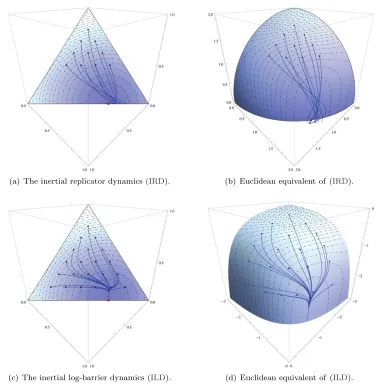
Example
2.3 (
the inertial replicator dynamics
).
The Shahshahani kernel
θ
(
x
) =
x
log
x
has
θ
(
x
) = 1
/x
and
θ
(
x
) =
−
1
/x
2, so (ID) leads to the
inertial replicator
dynamics
(IRD)
x
¨
kα=
x
kαv
kα−
β
x
kβv
kβ+
1
2
x
kα˙
x
2kαx
2kα−
β
˙
x
2kβx
kβ−
η
x
˙
kα.
As we mentioned in the introduction, the only notable difference between (IRD) and
the second-order replicator dynamics of exponential learning (RD
2) is the factor 1
/
2
in the right-hand side (RHS) of (IRD) (the friction term
η
x
˙
is not important for this
comparison). Despite the innocuous character of this scaling-like factor,
14we shall see
in the following section that (IRD) and (RD
2) behave in drastically different ways.
Example
2.4 (
the inertial log-barrier dynamics
).
The log-barrier kernel
θ
(
x
) =
−
log
x
has
θ
(
x
) = 1
/x
2and
θ
(
x
) =
−
2
/x
3, so we obtain the
inertial log-barrier
dynamics
(ILD)
x
¨
kα=
x
2kαv
kα−
r
−2kβ
x
2kβv
kβ+
x
2kα˙
x
2kαx
3kα−
r
−2 k
β
˙
x
2kβx
kβ−
η
x
˙
kα,
where
r
2k=
kβx
2kβ. The first-order analogue of these dynamics—namely, the system
˙
x
kα=
x
2kα(
v
kα−
r
−2k kβx
2kβv
kβ)—has been studied extensively in the context of
linear programming and convex optimization [5,
9,
11,
14,
27], while its game-theoretic
properties are discussed in [30].
3. Basic properties and well-posedness.
In this section, we examine the
energy dissipation and well-posedness properties of (ID). For convenience, we will
work with the single-agent version of the dynamics (ID) with
v
=
∇
Φ for some
Lipschitz continuous and sufficiently smooth function Φ on
X
.
153.1. Friction and dissipation of energy.
We begin by showing that the
sys-tem’s total energy
(3.1)
E
(
x,
x
˙
) =
1
2
x
˙
2
−
Φ(
x
)
is dissipated along the inertial dynamics (ID) for
η >
0 (or is a constant of motion in
the frictionless case
η
= 0).
Proposition 3.1.
The total energy
E
(
x,
x
˙
)
is nonincreasing along any interior
solution orbit of
(ID)
; specifically,
(3.2)
E
˙
=
−
2
ηK
=
−
η
x
˙
2
,
where
K
=
12x
˙
2
is the system’s kinetic energy.
14It is tempting to interpret the factor 1/2 in (IRD) as a change of time with respect to (RD
2),
but the presence of ˙x2precludes as much.
15Here and in what follows, it will be convenient to assume that Φ is defined on an open
neigh-borhood ofX. This assumption facilitates the use of standard coordinates for calculations, but none of our results depend on this device.
Proof
. By differentiating (3.1) along ˙
x
(
t
), we readily obtain
˙
E
=
∇
x˙E
=
1
2
∇
x˙x,
˙
x
˙
− ∇
x˙Φ =
∇
x˙x,
˙
x
˙
−
d
Φ
|
x
˙
=
D
2x
Dt
2,
x
˙
−
grad Φ
,
x
˙
=
grad Φ
−
η
x,
˙
x
˙
−
grad Φ
,
x
˙
=
−
η
x,
˙
x
˙
=
−
2
ηK,
(3.3)
where we used the metric compatibility (A.12) of
∇
in the first line and the definition
of the dynamics (ID) in the second.
Proposition
3.1
shows that, for
η >
0, the system’s total energy
E
=
K
−
Φ is
a Lyapunov function for (ID); by contrast, in first-order HR gradient flows [5,
11], it
is the maximization objective Φ that acts as a Lyapunov function. As such, in the
second-order context of (ID), it will be important to show that the system’s kinetic
energy eventually vanishes—so that Φ becomes an “asymptotic” Lyapunov function.
To that end, we have the following proposition.
Proposition 3.2.
Let
x
(
t
)
be a solution trajectory of
(ID)
that is defined for all
t
≥
0
. If
η >
0
, then
lim
t→∞x
˙
(
t
) = 0
.
To prove Proposition
3.2, we will require the following intermediate result.
Lemma 3.3.
Let
x
(
t
)
be an interior solution of
(ID)
that is defined for all
t
≥
0
.
If
η >
0
, the rate of change of the system’s kinetic energy is bounded from above for
all
t
≥
0
.
Proof
. By differentiating
K
with respect to time, we readily obtain
˙
K
=
∇
x˙K
=
D
2x
Dt
2,
x
˙
=
grad Φ
−
η
x,
˙
x
˙
=
d
Φ
|
x
˙
−
η
x
˙
2
=
β∂
Φ
∂x
βx
˙
β−
η
β
θ
βx
˙
2β≤
A
β
|
x
˙
β| −
ηB
β
˙
x
2β,
(3.4)
where
A
= sup
|
∂
βΦ
|
<
∞
and
B
= inf
{
θ
(
x
) :
x
∈
(0
,
1)
}
. With
A
finite and
B >
0 (on account of the Legendre properties of
θ
), the maximum value of the above
expression is (
n
+ 1)
A
2/
(4
ηB
), so ˙
K
is bounded from above.
Proof of Proposition
3.2. Let
E
(
t
) =
12x
˙
(
t
)
2
−
Φ(
x
(
t
)) be the system’s energy
at time
t
. Proposition
3.1
shows that ˙
E
=
−
η
x
˙
2
=
−
2
ηK
≤
0, so
E
(
t
) decreases to
some value
E
∗∈
R
; as a result, we also get
0∞K
(
s
)
ds
= (2
η
)
−1(
E
(0)
−
E
∗)
<
∞
.
This suggests that lim
t→∞K
(
t
) = 0, but since there exist positive integrable functions
which do not converge to 0 as
t
→ ∞
, our assertion does not yet follow.
Assume therefore that lim sup
t→∞K
(
t
) = 3
ε >
0. In that case, there exists by
continuity an increasing sequence of times
t
n→ ∞
such that
K
(
t
n)
>
2
ε
for all
n
. Accordingly, let
s
n= sup
{
t
:
t
≤
t
nand
K
(
t
)
< ε
}
: since
K
is integrable and
nonnegative, we also have
s
n→ ∞
(because lim inf
K
(
t
) = 0), so, by descending to a
subsequence of
t
n, we may assume without loss of generality that
s
n+1> t
nfor all
n
.
Hence, if we let
J
n= [
s
n, t
n], we have
(3.5)
∞0
K
(
s
)
ds
≥
∞
n=1
Jn
K
≥
ε
∞
n=1