Saeed Anwar
A thesis submitted for the degree of
Doctor of Philosophy
The Australian National University
October 2018
c
Copyright by Saeed Anwar 2018
I hereby declare that this submission is my own work (based on publications in collaboration with the co-authors where due acknowledgement is made) and that, to the best of my knowledge, it contains no material previously published or written by another person nor material which to a substantial extent has been accepted for the award of any other degree or diploma at ANU or any other educational institution, except where due acknowledgment has been made.
I also declare that all sources used in this thesis have been fully and properly cited.
First and foremost, I am very thankful to Allah “The Most Merciful”. After that, I would like to express my sincere gratitude to my panel chair and CVRG group leader, Prof. Fatih Porikli, for his guidance, motivation, and support throughout my Ph.D. It has been an absolute privilege to work with Fatih, and my Ph.D. would not have been possible without his enthusiasm for research. I am very thankful to you, professor, for treating me with kindness throughout this arduous journey, and for being immensely helpful in many ways both academic and personal matters. Your guidance has been instrumental in reducing my learning time.
I am equally grateful to my primary supervisor, Dr. Cong Phuoc Huynh. Thank you for giving me valuable pointers and ideas, shaping my research and carefully re-viewing all manuscripts that I produced during Ph.D. I am indebted to Dr. Cong for his continuous guidance and for his valuable time even after he moved to Amazon. I am very thankful to Cong for bearing with me during my Ph.D.
I would also like to thank the other researchers at Data61 (previously NICTA) and ANU for their feedback on my research during various seminars and reading groups. I am grateful to my colleagues at Data61 and ANU, past and present, who created an excellent research environment. Primarily, I would like to convey my gratitude to Dr. Khurram Aftab, Dr. Ahmed Sohaib (who introduced me to this unique opportunity), Dr. Salman H. Khan, Dr. Zeeshan Hayder, Dr. Thalaiyasingam Ajanthan, Dr. Arash Shahriari, Yusuf, Masoud, and Samitha. We had the very fruitful discussion about many aspects of life, science, and religion.
I graciously acknowledge and appreciate the financial support from the Aus-tralian National University, Data61 (previously NICTA) and the AusAus-tralian Govern-ment for my Ph.D. research. Their scholarships and generous travel grants have al-lowed me to focus on my research without having to worry about financial support. I am indebted to my teachers at the University of Peshawar, Heriot-watt University, University of Girona and University of Bourgogne. I am thankful to Ehsan, Hashim, and Wajid for supporting me during my master degree.
I owe a great deal to my family. I would like to express my gratitude to my family and friends. I want to thank, my father, Khurshid Anwar, and my mother, Mushtaq Begum, for their upbringing, financial support and countless prayers all through these years. I am also indebted to my sister, my brothers and my wife for their unconditional love and support. To my daughter, Ummy Aiman and my son,
Every day many images are taken by digital cameras, and people are demanding visually accurate and pleasing result. Noise and blur degrade images captured by modern cameras, and high-level vision tasks (such as segmentation, recognition, and tracking) require high-quality images. Therefore, image restoration specifically, im-age deblurring and imim-age denoising is a critical preprocessing step.
A fundamental problem in image deblurring is to recover reliably distinct spatial frequencies that have been suppressed by the blur kernel. Existing image deblurring techniques often rely on generic image priors that only help recover part of the fre-quency spectrum, such as the frequencies near the high-end. To this end, we pose the following specific questions: (i) Does class-specific information offer an advan-tage over existing generic priors for image quality restoration? (ii) If a class-specific prior exists, how should it be encoded into a deblurring framework to recover at-tenuated image frequencies? Throughout this work, we devise a class-specific prior based on the band-pass filter responses and incorporate it into a deblurring strat-egy. Specifically, we show that the subspace of band-pass filtered images and their intensity distributions serve as useful priors for recovering image frequencies.
Next, we present a novel image denoising algorithm that uses external, category specific image database. In contrast to existing noisy image restoration algorithms, our method selects clean image “support patches” similar to the noisy patch from an external database. We employ a content adaptive distribution model for each patch where we derive the parameters of the distribution from the support patches. Our objective function composed of a Gaussian fidelity term that imposes category specific information, and a low-rank term that encourages the similarity between the noisy and the support patches in a robust manner.
Finally, we propose to learn a fully-convolutional network model that consists of a Chain of Identity Mapping Modules (CIMM) for image denoising. The CIMM structure possesses two distinctive features that are important for the noise removal task. Firstly, each residual unit employs identity mappings as the skip connections and receives pre-activated input to preserve the gradient magnitude propagated in both the forward and backward directions. Secondly, by utilizing dilated kernels for the convolution layers in the residual branch, each neuron in the last convolution layer of each module can observe the full receptive field of the first layer.
Acknowledgements vii
Abstract ix
1 Introduction 1
1.1 Image Processing . . . 1
1.2 Image Restoration . . . 4
1.2.1 Image Deblurring . . . 5
1.2.1.1 Non-Blind Deblurring . . . 7
1.2.1.2 Blind Deblurring . . . 8
1.2.1.3 Limitation of Existing Deblurring Algorithms . . . 9
1.2.1.4 Our Contribution to Deblurring Task . . . 9
1.2.2 Image Denoising . . . 10
1.2.2.1 Limitation of Existing Denoising Algorithms . . . 11
1.2.2.2 Our Contributions to Denoising Task . . . 12
1.3 Thesis Outline . . . 13
1.4 Publications . . . 14
1.4.1 Published papers . . . 14
1.4.2 Under-review papers . . . 14
2 Background and Preliminaries 15 2.1 Image Deblurring . . . 15
2.1.1 Non-blind Deblurring . . . 15
2.1.1.1 Iterative Methods . . . 17
2.1.1.2 Image Priors . . . 18
2.1.2 Blind Deblurring . . . 19
2.1.2.1 Edge Priors . . . 20
2.1.2.2 Probabilistic Priors . . . 23
2.1.2.3 Patch Priors . . . 24
2.1.2.4 Class-specific Priors . . . 25
2.1.2.5 Learning with Neural Networks . . . 27
2.2 Image Denoising . . . 28
2.2.1 Image Filtering . . . 28
2.2.1.1 Linear Filtering . . . 28
2.2.1.2 Median Filtering . . . 29
2.2.1.3 Denoising via Local Statistics . . . 30
2.2.1.4 Bilateral Filtering . . . 30
2.2.2 Methods using Local Structure Similarity . . . 30
2.2.2.1 Non-local Means . . . 31
2.2.2.2 Block Matching and Three Dimensional Filtering . . . . 31
2.2.2.3 Non-local Bayes . . . 33
2.2.2.4 Weighted Nuclear Norm Minimization . . . 33
2.2.2.5 Principal Component Analysis . . . 33
2.2.2.6 Dual Domain & Progressive Image Denoising . . . 34
2.2.3 External Denoising Methods . . . 34
2.2.3.1 Targeted Image Denoising . . . 35
2.2.3.2 Combined Image Denoising . . . 35
2.2.4 Learning Patch Statistics . . . 36
2.2.4.1 Denoising via Singular Value Decomposition . . . 36
2.2.4.2 Non-local Sparse Models . . . 36
2.2.4.3 Spatially Adaptive Iterative Singular Value Threshold-ing . . . 37
2.2.4.4 Gaussian Mixture Model priors . . . 37
2.2.4.5 Adaptive Image Denoising . . . 38
2.2.5 Convolutional Neural Networks . . . 39
2.2.5.1 Cascade of Shrinkage Fields . . . 39
2.2.5.2 Trainable Nonlinear Reaction-Diffusion . . . 39
2.2.5.3 DnCNN & IrCNN . . . 40
2.2.5.4 Non-local Color Image Denoising with CNN . . . 41
2.2.5.5 FormResNet . . . 41
2.2.5.6 Wavelet Domain Deep Network . . . 41
2.3 Summary . . . 42
3 Image Deblurring with a Class-Specific Prior 43 3.1 Introduction . . . 43
3.2 Problem Formulation . . . 48
3.2.1 Image Prior . . . 48
3.2.2 Objective Function . . . 49
3.3 Deblurring Framework . . . 50
3.3.1 Estimatingwgivenxandk . . . 50
3.3.2 Latent Image Estimation . . . 50
3.3.4 Implementation . . . 53
3.3.5 Extension to Color Images . . . 55
3.4 Results and Discussion . . . 56
3.4.1 Datasets and Experimental Settings . . . 56
3.4.2 Ablation Study . . . 57
3.4.2.1 Effectiveness of the Prior . . . 57
3.4.2.2 Influence of Data Fidelity Terms on Kernel Estimation . 59 3.4.2.3 Influence of the Dataset Size . . . 59
3.4.2.4 Choice of the Training Class . . . 60
3.4.2.5 Schedule of the Prior Weightβ . . . 61
3.4.2.6 Number of Bandpass Filters . . . 61
3.4.2.7 Reconstruction Error of the Latent Image . . . 62
3.4.2.8 Grayscale vs. Color . . . 63
3.4.2.9 Convergence . . . 63
3.4.2.10 Runtime . . . 65
3.4.2.11 Real-world Images . . . 65
3.4.2.12 Reconstruction of a Cat Image . . . 66
3.4.2.13 Distribution of weights of filtered training images . . . 67
3.4.3 Comparisons with Generic Image Deblurring . . . 68
3.4.4 Comparison with Exemplar-based Methods . . . 77
3.5 Discussion . . . 80
4 Category-Specific Object Image Denoising 83 4.1 Introduction . . . 84
4.2 Denoising Problem Formulation . . . 85
4.2.1 Support patch search . . . 86
4.2.2 Transform domain formulation . . . 87
4.2.3 Data Fidelity . . . 88
4.2.4 Support Patch Group Membership . . . 88
4.2.5 Low-rank Constraint . . . 89
4.3 Optimization . . . 89
4.3.1 Patch Denoising . . . 90
4.3.1.1 Update ofαi with FixedMi . . . 91
4.3.1.2 Update ofMi with Fixed αi . . . 91
4.3.2 Recovering Latent Images . . . 91
4.3.3 Implementation Details . . . 92
4.4 Experiments . . . 94
4.4.1 Datasets and Parameter Settings . . . 94
4.4.3 Influence of the number of support patches . . . 96
4.4.4 Relative Importance of the Priors . . . 96
4.4.5 Runtime Comparisons . . . 96
4.4.6 Role of the External Image Category . . . 97
4.4.7 Sensitivity to Pose Variations . . . 102
4.4.8 Comparisons with Internal Denoising Methods . . . 102
4.4.9 Comparisons with External Denoising Methods . . . 103
4.4.10 Robustness to Misalignments and Rotations . . . 104
4.4.11 Extension to Color Images . . . 104
4.5 Discussion . . . 104
5 Chaining Identity Mapping Modules for Image Denoising 107 5.1 Introduction . . . 107
5.2 Chain of Identity Mapping Modules . . . 109
5.2.1 Network Design . . . 110
5.2.1.1 Network Elements . . . 110
5.2.1.2 Justification of the Design . . . 111
5.2.1.3 Our Formulation . . . 112
5.2.2 Learning to Denoise . . . 112
5.3 Experiments . . . 113
5.3.1 Benchmark Datasets and Baseline Methods . . . 113
5.3.2 Training Details . . . 113
5.3.3 Boosting Denoising Performance . . . 114
5.3.4 Identity Mapping Modules . . . 114
5.3.5 Ablation Study . . . 114
5.3.5.1 Influence of the Patch Size . . . 114
5.3.5.2 Number of Modules . . . 115
5.3.5.3 Kernel Dilation and Number of Layers . . . 115
5.3.5.4 Combination of Kernel Dilation, Identity Connection and Boosting . . . 116
5.3.6 Comparisons . . . 117
5.3.6.1 Classical Images . . . 119
5.3.6.2 BSD68 Dataset . . . 121
5.3.6.3 Color Image Denoising . . . 121
5.3.6.4 Darmstadt Noise Dataset: Real-world Images . . . 122
6 Conclusion and Future Work 127
6.1 Conclusion . . . 127 6.2 Future Directions . . . 129
1.1 Examples of different kind of artifacts found in images. . . 2 1.2 A degradation model where the input image is corrupted by first
pass-ing the image into a filter and then addpass-ing noise to it. . . 4 1.3 An example of cat image blurred by eight different blur kernels. The
blur kernels are shown in the left top corner of each image. The blur kernel values are positive and normalized so that the sum of its ele-ments is unity. . . 6
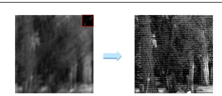
1.4 Examples of grayscale and color images for noise variances of 10, 30, 50 and 75. . . 6 1.5 Example result of image deblurring. Given the blurry image on the
left, we need to restore the original image shown on the right. . . 7 1.6 Visual artifacts caused by the direct inverse filter. On the left: blurred
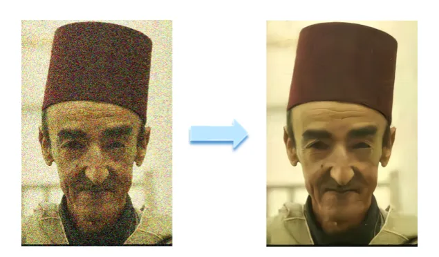
image and PSF and on the right output of inverse filtering. . . 8 1.7 An example of image denoising. Given the noisy image on the left, we
need to restore the original image shown on the right. . . 10
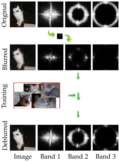
2.1 The neural blind deblurring system of [Chakrabarti, 2016]. The blurry patch is decomposed into multiple frequency “bands”, where Lis low pass, B1,B2 are band-pass and H stands for high-pass frequency com-ponents. Furthermore, DFT means discrete Fourier transform and IDFT stands for inverse discrete Fourier transform. . . 27
2.2 Example of grouping patches from noisy images. Each image shows a reference patch “R” (in red) and similar looking patches (in blue). . . . 32
2.3 BM3D framework. The process is repeated as indicated by the dashed lines. . . 32
2.4 A general framework for the external denoising methods. . . 34 2.5 The architecture of the TRND network. k1i is the set of linear kernels,
y0 the degraded image,x is the groundtruth image and α1 is strength of the term. . . 40 2.6 The architecture of the DnCNN and IrCNN network. . . 40
2.7 FormResNet Proposed network structure. . . 41
3.1 Recovering spatial frequencies that have been suppressed by a blur kernel using band-pass frequency components from the training data. . 45
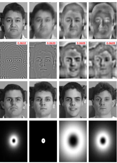
3.2 A visual demonstration of the proposed prior. Top row (from left to right): original (ground-truth) image x∗, input blurred image y, the image reconstructed by the weighted combination of all the filtered training images, and the absolute difference kx−x∗k. Second row (from left to right): the four most important filtered training images sorted by the descending order of their weights (shown in the inset). Third row: the training images corresponding to those in the second row. Fourth row: the bandpass filters (shown in the frequency domain) involved in the filtered training images in the second row. . . 47
3.3 Latent images and kernels recovered by our method without (third column) and with the proposed prior (fourth column). . . 57
3.4 Influence of the data fidelity term in the objective function on the ker-nel estimate. A pair of PSNR/SSIM error metrics is shown for each kernel estimate in the sub-figures (d)–(f). (a) ground-truth image, (b) blurred image, (c) ground-truth kernel, (d) estimated kernel with the intensity term only, (e) estimated kernel with the gradient term only, (f) estimated kernel with both terms. . . 60
3.5 The relative reconstruction errors (averaged over 80 test images) for the INRIA person [Dalal and Triggs, 2005], the CMU-PIE [Sim et al., 2002] and the Yale-B [Georghiades et al., 2001] datasets. . . 62
3.6 The convergence of the iterative algorithm. The image and kernel sim-ilarity between the estimated and the ground-truth are measured in terms of the SSIM. . . 64
3.7 Estimated kernels for the sample image in Figure 3.6 at different scales. As visible, the kernel becomes progressively more similar to the ground-truth at finer resolutions. . . 64
3.8 Deblurring a real-world image (with no known ground-truth) from the dataset in [Shi et al., 2014]. . . 65
3.9 Deblurring results for real input images from [Pan et al., 2014a], where the one in the first row contains noise and saturated pixels. . . 66
3.10 The reconstruction of a cat image, by taking the weighted combination of all the filtered training images from the Cat dataset. From left to right: blurred input image, important filtered training images, and reconstructed image. . . 67
3.12 Results for a sample image from the Car dataset in [Krause et al., 2013]. The restored image from our method has more legible text on the li-cense plate compared to the other methods. . . 71
3.13 Comparison of several methods on a sample image selected from the INRIA dataset[Dalal and Triggs, 2005]. Our method successfully re-covers parts of the image with a significant resemblance to the ground-truth, including the pedestrians and the bus in the background. Our estimated kernel is also the most accurate among all the methods. . . . 71
3.14 Comparisons on a sample image from the Cat dataset[Zhang et al., 2008]. Our method recovers fine texture around the neck, mouth, and whiskers, which cannot be accurately reproduced by the others. . . 72
3.15 Comparisons on a sample image with strong edges and a blurred back-ground, selected from the ETHZ Shape Classes dataset [Ferrari et al., 2010]. The visual quality,e.g. sharpness of the text on the label, repro-duced by our method is par to the best one among the other methods, i.e.[Sun et al., 2013]. . . 72 3.16 Comparisons on a sample image with rich textures, selected from the
ETHZ Shape Classes dataset [Ferrari et al., 2010]. On a magnified view, the image our method recovers is sharper than those generated by most of the methods, and comparable to the best,i.e. of [Xu et al., 2013], while exhibiting a less degree of ringing artifacts. . . 73 3.17 Comparisons on a face image selected from the CMU PIE dataset [Sim
et al., 2002]. Although our deblurred image appears to be similar to those produced some other methods, its intensity profile (on the face) is richer than the other methods. . . 73 3.18 Comparisons on a sample face image selected from the Yale-B dataset[Georghiades
et al., 2001]. The image we recover is more natural and contains less ringing and exaggerated contrast artifacts. Our estimated kernel is also the closest to the ground-truth. . . 74 3.19 Comparisons on a sample image from the FEI dataset[Thomaz and
Giraldi, 2010]. Differences can be better seen in magnified view. . . 74
3.20 Intensity profiles (corresponding to pixel row 55) of the deblurred im-ages produced by our method and others. The input blurred image is given in Figure 3.18b. The red trace in each subplot shows the ground-truth profile. . . 75 3.21 Comparison with [Zhang et al., 2011]. (a) Ground-truth image, (b)
3.22 Comparison to [Hacohen et al., 2013]’s on a blurred image taken from their paper. . . 78 3.23 Deblurring of an image containing foreground text and complex
back-ground. (a) Ground-truth (sharp) image, (b) blurred image, (c) deblur-ring results by [Pan et al., 2014b], (d) our results (zoom in to see the differences). . . 79 3.24 Results for an image provided by [Pan et al., 2014a]. First column:
ground-truth image, second column: blurred images and original blur kernels (at the top left corners of the images), third column: deblurred images and estimated kernels by [Pan et al., 2014a], fourth column: our results. . . 80
4.1 Denoising results of two sample images from face and cat categories. As visible, by using the same category support dataset we generate higher PSNR scores-shown in red (best viewed in high-resolution). . . . 84 4.2 Searching and selecting support patches for a given noisy patch yi.
Candidate images similar to the noisy image (measured by SSIM) are selected from the given database. Subsequently, in each candidate im-age, we search for patches that are similar to the noisy patch,i.e. within a Euclidean distance of τ from yi. The search is restricted to a
lo-cal window in each candidate image. Finally, among the remaining patches, only the nearest neighbors toyi are retained for denoising. . . 86
4.3 Denoising accuracy (in PSNR) at noise standard deviationsσn=30 and
σn=50. Left: Our method is robust to the changes in the dataset size,
which has a low impact on the results. Right: Increasing the number of support patches slightly degrades the denoising results. . . 95 4.4 Denoising results produced by different methods for a face image in
a profile view from the FEI face dataset [Thomaz and Giraldi, 2010] when σn = 30. Our method can denoise the input image even with
a different pose from those in the noise-free dataset (Differences are better viewed with high-resolution display). . . 97 4.5 Denoising results produced by different methods for a face image
se-lected from the Gore dataset [Peng et al., 2012] when σn = 20. Our
method is able to denoise the face image even with a different pose from those in the noise-free dataset. . . 98 4.6 Visual denoising results produced forσn=50, by several methods for
4.7 Denoising results achieved by various methods for a sample image with a noise standard deviation σn = 30. The ground truth image is
from the Gore dataset [Peng et al., 2012]. . . 100
4.8 Visual denoising results for a texture image selected from the Multi-view dataset [Hirschmüller and Scharstein, 2007] whereσn= 50. Our
method can recover much more texture details than the others (please zoom-in to see details). . . 101
4.9 Denoising results for different methods from the dataset in [Zhang et al., 2008] when σn = 50. The top two rows show the candidate
images from the dataset that are most similar to the noisy image. . . 101
4.10 Comparison of a few denoising methods on color images from the datasets in [Hirschmüller and Scharstein, 2007] and [Thomaz and Gi-raldi, 2010], where the noise standard deviations are σn = 20 and
σn = 80, respectively. Our method can recover much more details
than the others. . . 102
5.1 Denoising results for an image corrupted by the Gaussian noise with
σ = 50. Our result has the best PSNR score, and unlike other meth-ods, it does not have over-smoothing or over-contrasting artifacts. Best viewed in color on high-res display. . . 108
5.2 The proposed network architecture, which consists of multiple mod-ules with similar structures. Each module is composed of a series of pre-activation-convolution layer pairs. . . 110
5.3 Denoising quality comparison on a sample image with strong edges and texture, selected from classical image set for noise level σn = 50.
The visual quality, i.e. sharpness of the edges on the wings and small textures reproduced by our method is the better than others. . . 117
5.4 Comparison on a sample image from BSD68 dataset [Roth and Black, 2009] for σn = 50. Our network is able to recover fine textures in the
background and on the castle, while other methods cannot reproduce such textures accurately. . . 118
5.5 Denoising performance for state-of-the-art versus the proposed method on sample color images from the dataset in [Roth and Black, 2009], where the noise standard deviation σn is 50. The image we recover
5.6 A sample color image with rich textures, selected from the BSD68 dataset [Roth and Black, 2009] for σn = 25. On a magnified view,
the image our network recovers is sharper than those generated by most of the methods . . . 120 5.7 Real images from Darmstadt Noise Dataset (DND) benchmark for
dif-ferent denoising algorithms [Plötz and Roth, 2017]. . . 123 5.8 Two real images from [Zhang et al., 2017a] denoised by our noise level
3.1 A comparison of the accuracy achieved by our deblurring framework on all the mentioned datasets with and without the proposed prior. . . 58 3.2 Influence of intensity and gradient fidelity terms on the deblurring
results. . . 58 3.3 Deblurring performance (in PSNR) on the CMU PIE dataset for
differ-ent numbers of training images. . . 59 3.4 Deblurring performance (in PSNR) for different classes of the blurred
input image and the external training datasets. The PSNR is signifi-cantly higher when the external dataset matches the input image cate-gory. . . 61 3.5 The average image accuracy (in PSNR) achieved with a constant prior
weightβwhen our algorithm is evaluated on the Person dataset [Dalal and Triggs, 2005]. . . 61 3.6 The average accuracy of the deblurred image (in PNSR) for the Person
dataset [Dalal and Triggs, 2005], with respect to different numbers of bandpass filters M. . . 62 3.7 A comparison of the image and kernel accuracy (in PSNR) obtained
using greyscale vs. colour input images. The results are reported for the INRIA person dataset [Dalal and Triggs, 2005]. . . 63 3.8 The accuracy of the deblurred images, measured by SSIM and PSNR.
The missing results, indicated by “-”, occurs when the respective method is not capable of dealing with the low resolution of the input images. Best results are in bold. . . 69 3.9 The similarity between the estimated kernel to the ground-truth,
mea-sured by SSIM and PSNR. The missing results, indicated by “-”, occurs when the respective method is not capable of dealing with the low res-olution of the input images. Best results are in bold. . . 70
4.1 Run-time comparisons (in seconds) on a test image of size 304×228. . 95 4.2 Denoising performance (in PSNR) when using different image
gory datasets. The PSNR is maximal when the external dataset cate-gory matches the noisy image catecate-gory. . . 96
4.3 Performance comparison between our method and internal denoising techniques on several datasets, in terms of PSNR (in dB). . . 98 4.4 Performance comparison between our method and external denoising
techniques on several datasets, in terms of PSNR (in dB). . . 99 4.5 Denoising performance in PNSR (dB) on color images for noise levels
σn=30, 50, 70, 80, 100. Best results are in bold. . . 99
5.1 Detailed architecture of an identity mapping module. . . 115 5.2 Denoising performance (in PSNR) on the BSD68 dataset [Roth and
Black, 2009] for different sizes of training input patches for σn = 25,
keeping all other parameters constant. . . 115 5.3 The average PSNR accuracy of the denoised images for the BSD68
dataset, with respect to different number of modules M. The higher the number of modules, the higher is the accuracy. . . 115 5.4 Denoising performance for different network settings to dissect the
relationship between kernel dilation, number of layers and receptive field. . . 116 5.5 PSNR reported on the BSD68 dataset for σn = 25 when different
fea-tures are added to the DnCNN baseline (first row). . . 116 5.6 Comparisons with state-of-the-art methods on BSD68 with σn = 50,
and BSD100 with σn = 25. The results of [Bae et al., 2017] and [Jiao
et al., 2017] are taken from their respective papers. . . 117 5.7 Performance comparison between image denoising algorithms on widely
used classical images, in terms of PSNR (in dB). The best results are highlighted with bold red color while the blue color represents the second best denoising results. . . 119 5.8 Performance comparison between our method and existing algorithms
on the grayscale version of the BSD68 dataset [Roth and Black, 2009]. The missing denoising results, indicated by “-”, occurs when the method is not trained to deal with the input noisy images. . . 120 5.9 The similarity between the denoised color images and the
ground-truth color images of the BSD68 dataset for our method and exist-ing algorithms measured by PSNR (in dB) reported for noise levels of
σ=15, 25, and 50. . . 121 5.10 Mean PSNR and SSIM of the denoising methods evaluated on the real
1 Deblurring with the class-specific prior. . . 54 2 Denoising with category-specific support patches . . . 93
Introduction
Everything you can imagine is real.
Pablo Picasso
In the current digital age, camera-based equipments, such as smartphones and hand-held cameras allow people to capture a significant amount of image data and help share it through social media. However, the image data quality suffers from var-ious forms of artifacts and degradations such as blur (motion, defocusetc.) and noise (Gaussian, speckle, thermaletc.). The process of undoing the artifacts and recovering image details is termed as image restoration. Image restoration is a challenging and an ill-posed problem. However, we examine whether it is possible to procure more image contents to recover missing or corrupted observed image details. Fortunately, the amount of data available in our modern digital age changes the way we approach recent problems. Exemplar-based methods and learning methods are emerging and further improving the quality of image restoration tasks. For example, class-specific denoising methods are becoming popular for removing corrupted pixels and en-hancing the image quality. Similarly, exemplar-based image deblurring is introduced recently to demonstrate that large training sets provide superior performance. Before delving into the image restoration techniques in this thesis, we will briefly discuss common image artifacts and corresponding image enhancement techniques.
1
.
1
Image Processing
Image processing is used to preprocess images into a suitable form for tasks such as computational photography, recognition, and classification. Computer vision appli-cations require utmost care in designing the image enhancement stages to achieve desirable results. Examples of image processing are color correction, color balanc-ing, sharpenbalanc-ing, warpbalanc-ing, geometric transformations, removing unwanted objects, removing blur and noise reduction.
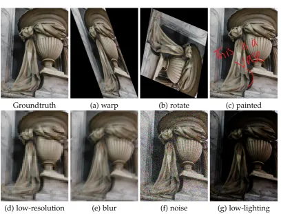
Groundtruth (a) warp (b) rotate (c) painted
[image:28.595.77.486.103.413.2](d) low-resolution (e) blur (f) noise (g) low-lighting
Figure 1.1: Examples of different kind of artifacts found in images.
Color correction [Rizzi et al., 2003; Vrhel and Trussell, 1992] means to modify the color of an input image so that its colorimetric properties are similar to those of a target image. Color is a vital cue topic in computer vision, human-computer interaction and feature extraction applications. The colors present in the images are due to intrinsic properties of the objects and the light source. The ability to filtered out the effects of the light source can account for color correction and is called color constancy.
Similarly, image warping [Wolberg, 1990; Glasbey and Mardia, 1998] is the pro-cess of mapping a source image into a destination image and is used for the correc-tion of geometric distorcorrec-tions due to imperfect imaging sensors. Sometimes artifacts like pincushion or barrel distortion are introduced by camera lenses, while other distortions are also possible such as projective distortions introduced by perspective views. The process of removing these geometric distortions from an image is known as image warping in computer vision.
et al., 2004]. This line of research is prevalent in recent years and is helpful in many applications such as recovering images from overlayse.g. scratches, and text, remov-ing unwanted objects and disocclussion in image-based renderremov-ing. Similarly, image compositing and matting techniques are for editing and enhancing visual effects of images. The process of extracting an object from an image foreground is known as matting while putting in another it into the image is called compositing.
Moreover, image super-resolution [Freeman et al., 2002; Kim et al., 2016a] refers to the process of obtaining a high-resolution image from a low-resolution image. This line of research has been very active over recent years, boosted by numerous applications: Iris recognition, medical imaging, fingerprint image processing, text image enhancement and satellite imagingetc.
Further, the act of recovering a clean signal from a blurry one is referred as image deconvolution or image deblurring [Fish et al., 1995; Ayers and Dainty, 1988]. It is well studied for decades and is useful in many fields of image processing such as robotic vision, surveillance, object segmentation and object recognition etc. We present more on image deblurring in Section 1.2.2
The removal of random fluctuations of the pixels of an image is known as image denoising [Lee, 1980; Tikhonov et al., 1977]. Image denoising is a preprocessing step in many areas of computer visione.g. medical imaging, satellite imaging, ultrasound imaging, infrared imaging and astronomical images etc. We discuss denoising in detail in the Section 1.2.2
In image processing, segmentation [Shi and Malik, 2000; Haralick and Shapiro, 1985] means partitioning of an image into many segments. More specifically, seg-mentation is the process of assigning the same label to the pixels that have specific similar properties in an image. Segmentation aims to simplify and modify the rep-resentation of an image into the more meaningful way which is straightforward to investigate. Commonly, segmentation is employed in locating objects and boundaries in an image.
Another worth mentioning image processing technique is edge detection [Perona and Malik, 1990; Canny, 1987]. Edge detection aims to identify the boundaries or sets of pixels in an image where the pixels of an image change abruptly or has discontinuities. Edge detection is useful in many applications such as segmentation, data extractionetc.
Figure 1.2: A degradation model where the input image is corrupted by first passing the image into a filter and then adding noise to it.
image from a degraded or corrupted one, while on the other hand, image enhance-ment seeks to the improve the perceptual quality of the image. Notably, the image restoration aims to precisely recover the original image even if the outcome may not be perceptually pleasing. While the image enhancement goal is to improve the visual quality of the picture, irrelevant whether the original signal becomes unwarranted. As a result, image restoration requires typically a model that describes the image formation process that how it is corrupted. However, image enhancement does not necessarily demand a model that gives the desired output. The respective underlying goals of image restoration and image enhancement is different; yet, there do exist a significant overlap between the two methods. Figure 1.1 shows images with different kinds of artifacts. In the next section, we introduce the image restoration tasks, ad-dressed in this thesis and show in subsequent chapters how they can be formulated using external datasets.
1
.
2
Image Restoration
Image restoration is an old classical problem where the aim is to recover the original clean signal from its degraded observation. Although this problem is very old and well-studied, still it is relevant in many fields e.g. medical imaging, surveillance, robotic visionetc.
To this end, we consider a simple image degradation model. Figure 1.2 is an example degradation model. The image captured using the camera is a degraded version of the original scene due to various factors such as limitations of the digital camera system or external influencee.g. environment and human hands movement. The degradation model shown in Figure 1.2 is linear; however, more complex degra-dations models can also be found.
and then further degraded by the noise, resulting in final blurry, noisy output image. The blurring filter is also known as point spread function (PSF) or blur kernel. The blur kernel can be either uniformi.e. same blur kernel is convolved with every pixel of the image, or non-uniformi.e. different blur kernels are applied on different pixels in the same image. Some common types of blur are motion blur and defocus blur.
In addition to blur, the noisenplays a role in degrading the image quality as well by randomly changing the intensity of image pixels. Common examples of noise are salt & pepper noise, speckle noise, shot noise, Gaussian noise and quantization noise. The characteristics of each noise mentioned arise from their respective noise source. Mathematically, Figure 1.2 can be modeled as
vec(y) =Kvec(x) +vec(n), (1.1)
where vec is an operator to convert a matrix to its vector form, xis the original un-corrupted image while vec(x) ∈ Rm. Similarly, y is the captured degraded image
while vec(y)∈ Rm. Kis the transformation matrix andnis the random noise. Image
restoration aims to recover the original uncorrupted imagexfrom the degraded ver-siony. If the noise in Equation 1.1 becomes zeroi.e.n= 0, then the image restoration problem becomes image deblurring problem, and the observed image is termed as a blurry image. Figure 1.3 shows a cat image blurred by different eight blur kernels. On the other hand, if the transformation operator becomes identity, i.e. K = I, the problem reduces to image denoising one. Figure 1.4 shows gray and color images for Gaussian at different noise levels. In this thesis, we are tacking the image de-noising and image deblurring problems individually as opposed to adding both the degradation to a single image.
1.2.1 Image Deblurring
Figure 1.3: An example of cat image blurred by eight different blur kernels. The blur kernels are shown in the left top corner of each image. The blur kernel values are positive and normalized so that the sum of its elements is unity.
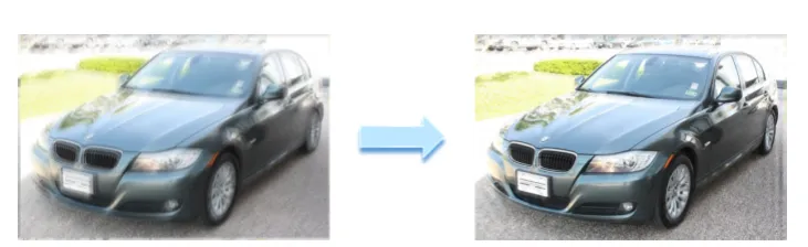
Figure 1.5: Example result of image deblurring. Given the blurry image on the left, we need to restore the original image shown on the right.
1.2.1.1 Non-Blind Deblurring
In non-blind deblurring, the aim is to recover the original unblurred image under the assumption that the blur kernel is known beforehand. In non-blind deblurring, the objective is to reduce the effect of inherent problems such as ringing artifacts, noise suppression, and increasing efficiency. Theoretically, a blurry image is modeled as a filtered version of the latent image and can be formulated as
y=k∗x, (1.2)
where k is the point spread function/blur kernel and “∗” is the convolutional op-erator. In image deblurring, for the sake of ease, computations are performed in frequency domain, as the convolution theorem states that Fourier transform F of a convolution is the element-wise multiplication, hence,
F(y) =F(k)·F(x), (1.3)
in simple case, the latent image x can be recovered by inverting the convolution process and can be expressed as
F(x) =F(y)/F(k), (1.4)
Figure 1.6: Visual artifacts caused by the direct inverse filter. On the left: blurred image and PSF and on the right output of inverse filtering.
and result in more complex forms.
Usually, image deblurring algorithms minimize two expressions: the data fidelity term and the prior term (also known as regularization). The data fidelity term cor-responds to likelihood in probability and minimizes the difference between the con-volved latent image and the blurry image. Commonly, the probability likelihood is equated to the distance functioni.e. the`2-norm
The regularization or prior term is different for different deblurring methodse.g. some methods apply sparsity, and others use incorporate edges in the prior. The prior term constrains the latent image x. A balancing weight is used between the data fidelity and prior terms. In Chapter 2, we discuss state-of-the-art non-blind deblurring methods with their respective strengths and weakness.
1.2.1.2 Blind Deblurring
Blind deblurring techniques require prior assumptions on the blur kernelkand the latent image x. Blind deblurring solves the problem of motion deblurring by esti-mating both the blur kernel f and the latent imagex. Numerous methods estimate the blur kernel and the latent image in an alternating optimization scheme, for ex-ample, [Pan et al., 2014a; Xu et al., 2013]. Blind deblurring is more difficult than non-blind deblurring because of more unknownsi.e. the blur kernelkand the latent imagex. Defining criteria for optimization is quite difficult as different blur kernels
kcan be estimated depending on the values of latent imagexand noise n.
the gradients or intensity of the latent image and the blur kernel. In Chapter 2, we examine state-of-the-art blind deblurring approaches concerning their model design and solver construction.
Image deblurring also moved from generic methods to more specific image type deblurring. Examples of specific types are domain knowledge [Pan et al., 2014a], specific-priors [Sun et al., 2014a] and CNN [Sun et al., 2015]. Our contribution to image deblurring can be categorized as class-specific image deblurring. Detailed literature about the specific type image deblurring is provided in Chapter 2.
1.2.1.3 Limitation of Existing Deblurring Algorithms
In this section of the chapter, we point out some of the limitations of the existing deblurring methods, and in the next section, we present our contribution and how our methods avoid these limitations.
Existing image deblurring algorithms rely on the blurred image properties such as sparsity, sharp edges and heuristic filters. The sparsity priors may degenerate the solution, producing the delta blur kernel and latent image same as the blurred image. Similarly, a typical failure mode for edge-based methods is dealing with the large-scale blur present in the image induced by the large blur kernels. Also, these methods rely on image filters which are unstable and can steer the image deblurring approach to wrong solutions. However, a major problem in image deblurring is to restore distinct spatial frequencies which have been attenuated by the blurring kernel. Existing techniques usually rely on generic image priors. But, these priors only help recover part of the frequency spectrum, such as the frequencies near the high-end.
1.2.1.4 Our Contribution to Deblurring Task
Here, we present novel algorithms for image deblurring and address the limitation of the previous algorithms. Our solutions are more effective in both qualitative and quantitative terms than the competitive methods. We give our contribution and pro-vide a brief overview that how the limitations of existing algorithms are addressed in the following paragraphs.
Figure 1.7: An example of image denoising. Given the noisy image on the left, we need to restore the original image shown on the right.
Specifically, we devise a prior based on the class-specific subspace of image intensity responses to band-pass filters. We learn that the aggregation of these subspaces across all frequency bands serves as a good class-specific prior for the restoration of frequencies that cannot be recovered with generic image priors.
1.2.2 Image Denoising
Image restoration becomes image denoising when K becomes an identity matrix, then Equation 1.1 can be rewritten in its classical image denoising form, given an additive i.i.d. Gaussian noise model,
vec(y) =vec(x) +vec(n), (1.5)
here, aim is to recover the clean image vec(x)∈ Rmfrom the noisy image vec(y)∈ Rm,
where vec(n) denotes the additive Gaussian noise with zero mean vector andσ2 vari-ancei.e. vec(n)∼ N(0,σ2)∈ Rm. Figure 1.7 is an example for image denoising.
In Chapter 4 and Chapter 5, we address the image denoising using external im-ages. Similar to image deblurring, image denoising is also studied for decades; how-ever, it is still relevant as it is useful in many other many computer vision tasks such as object detection, classification, and tracking. Image denoising is also useful in many other image processing tasks, for example, image deblurring, image super-resolution, and image inpainting.
variations and analog to digital conversion. All these can be modeled as Gaussian distributed noise. Similarly, the random arrival of the photon on image sensor causes shot noise, and typically, it is modeled as a Poisson distribution. This noise is very challenging in low light condition.
Image denoising literature reveals that the noise is usually modeled as Additive White Gaussian Noise (AWGN) with zero mean due to two main reasons. Firstly, the Gaussian noise is practically applicable to other types of noises such as shot noise, as this can also be transformed into Gaussian noise using Anscombe root transformation [Anscombe, 1948]. Secondly, Gaussian distribution can facilitate the mathematical analysis as it is mathematically tractable.
With recent advancement in image denoising, researchers have started to investi-gate external priors [Zoran and Weiss, 2011; Yue et al., 2015] as opposed to internal priors [Dabov et al., 2007b; Buades et al., 2005]. The difference between external and internal stems from the fact that whether the reference patches are taken from the im-age itself or an external database. It is observed that internal priors are efficient and computationally less expensive whereas external priors achieve better performance. Our method discussed in Chapter 4 falls in external prior category.
Recently, image denoising also started taking advantage of CNN. The input to the network is a noisy observation while the target is the original clean image. Many works [Zhang et al., 2017a; Lefkimmiatis, 2016] are presented in this category and are growing to date. In Chapter 5 of this thesis, we discuss image denoising using CNN, and aim to take advantage of CNN and use external images to train our network and learn an external prior in a systematic way.
1.2.2.1 Limitation of Existing Denoising Algorithms
Here, we present common limitation of the existing state-of-the-art methods and then conclude image denoising in this chapter with our contributions to overcome the mentioned limitations.
• Many state-of-the-art algorithms [Dabov et al., 2007b; Buades et al., 2005] rely
on internal self-similar patches to denoise the image. There are two main chal-lenges to image denoising: 1) internal image denoising methods are reaching its optimal performance [Levin and Nadler, 2011; Chatterjee and Milanfar, 2012], 2) the patches that rarely occur in the image, this “rare patch" effect causes the performance to decrease.
• Recently, CNN models are employed in image denoising. Undoubtedly, CNN
approaches still rely on the hyper-parameter settings, extensive fine-tuning, nonlocal self-similar patches, stage-wise training and learning noise pattern without exploiting the underlying structure. These elements impede the per-formance of CNN based image denoising.
1.2.2.2 Our Contributions to Denoising Task
To address and overcome the limitation of previous algorithms, we introduce new novel algorithms for image denoising. Our algorithms show superior performance compared to current competitive methods. In the following paragraphs, we list our contributions and state how we addressed the shortcomings of the competitive tech-niques.
• We present a novel category-specific image denoising algorithm that exploits
patch similarity between the input image and an external dataset only. We rely on external images in the same category as the input, to denoise textured regions. The external denoising component estimates the latent patches using the statistics, i.e. means and covariance matrices, of external patches, subject to a low-rank constraint. We show that our algorithm let us handle of a large variety of categories.
• We propose to learn a fully-convolutional network model for image
denois-ing. Our denoising model learns the noise with the underlying patch struc-ture. Also, we do not require stage-wise training and hyper-parameter setting. Our denoising network possesses distinctive features that are important for the noise removal task.
– Each residual unit employs identity mappings as the skip connections and receives pre-activated input to preserve the gradient magnitude propa-gated in both directions.
– Utilizing dilated kernels for the convolution layers in the residual branch, in other words within an identity mapping module, each neuron in the last convolution layer can observe the full receptive field of the first layer.
1
.
3
Thesis Outline
The structure of this thesis aims to provide the background and our contribution to image restoration as well as some future directions. The remaining chapters are summarized and organized as follows.
Chapter2
This chapter reviews the literature on image deblurring and image denoising. Fur-thermore, we also provide detail of state-of-the-art algorithms and associated theories in this chapter as well as explain preliminary hypotheses that are necessary to the understanding of the remaining episodes.
Chapter3
In this chapter, we devise a class-specific prior using the band-pass filter responses of clean, sharp images and incorporate it into a deblurring strategy. More specif-ically, we show that the subspace of band-pass filtered images and their intensity distributions serve as useful priors for recovering image frequencies that are difficult to recover by generic image priors. Here, we present the contribution from [Anwar et al., 2015] and its extended version [Anwar et al., 2018].
Chapter4
In this chapter, we present image denoising algorithm that uses external, category specific image databases. In contrast to existing external image denoising that searches for patches either from a generic database or the input image, we approximate the denoised image using external non-convex priors. In this chapter, we also highlight the relationship between noisy patches and its external counterparts and the effects of external reference patches on image denoising. This chapter is based on our pub-lished works [Anwar et al., 2017c] and [Anwar et al., 2017b].
Chapter5
Chapter6
In this final chapter of the thesis, we summarize of the works presented and discuss possible future research directions.
1
.
4
Publications
The contributions presented in this thesis have either been published or under review at the following venues.
1.4.1 Published papers
• S. Anwar, C. P. Huynh and F. Porikli,“Image Deblurring with a Class-Specific
Prior," IEEE Transactions on Pattern Analysis and Machine Intelligence (TPAMI), 2018
• S. Anwar, F. Porikli and C. P. Huynh, “ Category-Specific Object Image
Denois-ing," IEEE Transactions in Image Processing (TIP), 2017.
• S. Anwar, C. P. Huynh and F. Porikli,“Combined Internal and External
Category-Specific Image Denoising," British Machine Vision Conference (BMVC), 2017.
• S. Anwar, C. P. Huynh and F. Porikli,“Class-specific image deblurring," IEEE
International Conference on Computer Vision (ICCV), 2015.
1.4.2 Under-review papers
• S. Anwar, C. P. Huynh and F. Porikli, “Chaining Identity Mapping Modules for
Background and Preliminaries
In this chapter, we provide a comprehensive overview of the ideas and theories of image deblurring and image denoising, both these problems are long-standing and well-researched, with algorithms too many to discuss in this literature review. We here present an up-to-date overview of state-of-the-art and the main research trend to date. Our intention in this exposition is to provide the reader the background material about the work done in this area of research. More detailed and exhaustive literature for image deblurring, though not complete can be found in [Rajagopalan and Chellappa, 2014]. Similarly, for image denoising the choice to obtain an exhaus-tive overview of the algorithms would be [Lebrun et al., 2012] and [Milanfar, 2013].
In this section of the thesis, we first introduce the necessary methods for image deblurring methods which can be classified into 1) blind deblurring, and 2) non-blind deblurring. Next, in the remaining chapter, we present image denoising meth-ods which can be further categorized as 1) image filtering, 2) internal denoising, 3) external denoising and 4) learning methods.
2
.
1
Image Deblurring
As discussed previously, image deblurring can be divided into two main categories depending on the availability of the blur kernel i.e. non-blind and blind. In blind deblurring, one has to estimate both kernel and latent image while in non-blind case kernel is assumed to be available beforehand. In this section of the chapter, we first provide state-of-the-art non-blind image deblurring algorithms followed by blind ones.
2.1.1 Non-blind Deblurring
Successful and advanced state-of-the-art non-blind image deblurring dates back to late twentieth century. Examples of these methods are Wiener deblurring [Wiener,
1949], least square filtering by [Miller, 1970; Tikhonov et al., 1977], Richardson-Lucy [Richardson, 1972] and recursive Kalman [Woods and Ingle, 1981]. An exhaustive review of these early methods are provided in [Hunt, 1973].
Usually, non-blind approaches are composed of two expressions: the data fidelity term and the regularization term. The data fidelity term corresponds to likelihood in probability and minimizes the difference between the convolved latent imagexwith the blur kernelk(k∗x) and the blurry imageyand can be expressed as
Ed =Ψ(k∗x−y), (2.1)
where Ψ is a distance function and a common representation is the `2-norm i.e.
Ψ(·) =|| · ||2
2similar to [Wiener, 1949]. It is also known as Gaussian likelihood. The regularization or prior term is different for different methods and can be presented as Φ(x). The regularization is essential to avoid undesirable solution, constraining the solution space. When we have the data fidelity term and prior term, then the original unblurred image can be estimated by minimizing the following objective function
argmin x
||k∗x−y||2
2+αΦ(x), (2.2)
whereαis the balancing weight between the data fidelity and the prior terms. In the following sections, we discuss recent representative state-of-the-art non-blind meth-ods with their weaknesses, strengths, advantages, and disadvantages.
Two important regularizers used for non-blind deblurring are Gaussian and Tikhonov which are represented by Φ(x) = ||x||2 andΦ(x) = ||∇x||2, ( ∇ is the gradient op-erator applied on the intensity image) respectively. The Gaussian regularizer impose smoothness on the intensity values of image while Tikhonov enforces it on image gradients. After substituting the smoothness terms in Equation 2.2, we obtain
argmin x
||k∗x−y||2+
α||x||2, (2.3)
and
argmin x
||k∗x−y||2+α||∇x||2. (2.4)
An important benefit of the regularizers as mentioned above is the simplicity of the equations and the existence of a closed form solution. Consider a sparse matrix
form, then Equation 2.3 can be expressed as
E=||Kν(x)−ν(y)||2+α||ν(x)||2. (2.5)
Taking Equation 2.5 expanding and setting its derivative equal to zero with re-spect toν(x). The total energy of the system will become
E=ν(x)TKTKν(x)−2ν(y)TKν(x)
+αν(x)Tν(x) +ν(y)Tν(y).
(2.6)
To get the optimal solution, we take the derivative of Equation 2.6 and then set it to zero,
dE
dν(x) =2K
TK
ν(x)−2KTν(y) +2αν(x), (2.7)
KTKν(x)−KTν(y) +ν(x) =0, (2.8)
ν(x) = K
T
KTK+αI
ν(y), (2.9)
whereIis the identity matrix and having same size asKTK.
Next, we discuss the main non-blind deblurring methods, specifically, iterative methods and image prior algorithms.
2.1.1.1 Iterative Methods
Earlier, [Van Cittert, 1931] used an iterative solver for non-blind deblurring which can be represented as
xm+1 =xm+α(y−xm∗k), (2.10)
where m is the iteration index, α controls the speed of convergence and can be as-signed manually or selected automatically. The effect of [Van Cittert, 1931] is same as direct inverse filtering where no prior to the image is used to find the final unblurred image.
Another important and extensively used iterative method is [Richardson, 1972]. According to [Rajagopalan and Chellappa, 2014], the method of [Richardson, 1972] is similar to Poisson Maximum Likelihood without employing any regularization on
methods as it reduces the noise in the final unblurred image. Typically, the method is run for a large number of iterations to converge and to achieve the passable out-come, however, if stopped midway, the outcome may be inferior. The algorithm of [Richardson, 1972] can be written as
xm+1=xm
˜
k∗
y xm∗k
, (2.11)
where ˜k is the flipped/rotated version of k. A few works built upon [Richardson, 1972] to improve the performance. One such method is [Yuan et al., 2008], which administered bilateral filtering at multiple scales, making [Richardson, 1972] more efficient and robust to noise.
2.1.1.2 Image Priors
In recent years, more advanced non-blind deblurring methods are proposed to deal with the visual artifacts induced by the inaccurate and unreliable estimation of blur kernels. Image priors are introduced to suppress ringing artifacts and noise present in the image because of the imaging system or the blur kernels. A common under-standing about image priors is not to impose a higher penalty on wrong estimations to avoid deviated outcomes. In [Chan and Wong, 1998] the authors used sparse gra-dient priori.e.Φ(x) =||∇x||1, popularly termed as total variation or Laplacian prior. The∇is the concatenation of first-order horizontal and vertical derivative of the im-age intensitiesi.e.δxx,δyx. The purpose of the`1norm is to less penalize the deviant estimations as compared to`2normsi.e. Gaussian priors.
Similarly, [Shan et al., 2008] also proposed a piecewise continuous prior for Φ(x) as
Φ(x) =
λ1|∇ix|, τ≥ |∇ix|
λ2(∇ix)2+λ3, otherwise
where the parameterτis the agreed upon value where the natural priors are joined together. Similarly, indexiis the first order partial derivate in horizontal or vertical direction. λs are the constant parameters. [Levin et al., 2007] suggestedΦ(x) =||x||p, where p > 1 and termed it as hyper-Laplacian to achieve comparatively sharper details in final unblurred image. Furthermore, [Yang et al., 2009] used`1data fidelity term for suppression of impulse noise, written as
argmin x
||k∗x−y||1+α||∇x||1. (2.12)
impulse noise added to the image during formation. The choice of Gaussian and Laplacian likelihood is due to their robustness to noise and for being manageable in the formulation.
Other works to solve sparsely constrained non-blind deblurring include [Krish-nan and Fergus, 2009] where half-quadratic splitting method [Geman and Yang, 1995] is employed. Half-quadratic splitting method introduces auxiliary variables to relax the problem and consist of two steps. In the first step, the image patches are treated as constants while the auxiliary variables are updated. In the second step, the aux-iliary variables are kept fixed while the image patches are updated. The procedure alternatives for some iterations or when the difference between two consecutive steps is smaller than a threshold. The minimization problem is given by
min x
N
∑
i=1
α
2(k∗x−y) 2
i + J
∑
j=i
|fj∗x|p
, (2.13)
where iis the pixel index and fj are the first order derivatives, namely, f1 = [1,−1] and f2 = [1,−1]T.
Next, [Zoran and Weiss, 2011] used a Gaussian Mixture Model (GMM) while [Ha-cohen et al., 2013] incorporated a correspondence between the blurred and the clear reference image. In another work, [Sun et al., 2014b] investigated context-specific priors to transfer mid and high frequency details from example scenes for non-blind deconvolution. In our deblurring method provided in chapter 3, we use [Levin et al., 2007] in our non-blind step to obtain the final output of the algorithm.
2.1.2 Blind Deblurring
Blind deblurring is more difficult than non-blind deblurring because of the high di-mension of solution space and severely ill-posed problem as both blur kernelkand latent imagex need to be estimated. Blind deblurring methods assume strong con-straints on the latent image priorxand the blur kernel priork. Defining a criteria for optimization is quite different as different blur kernelskcan be estimated depending on the values ofxandn. Considerφ(k)is the prior for the blur kernel then it can be expressed as
argmin x,k
Ψ(k∗x−b) +α1Φ(x) +α2ϕ(k), (2.14)
represented asϕ(k) =||k||1. When all the three terms are combined we obtain
argmin x
||k∗x−b||2
2+α1||∇x||p+α2||k||1. (2.15)
The parameter p can take values of 1, 2 or between 0 and 1. The deblurring methods are composed of these terms with some alteration, or more terms are added to Equation 2.14. However, this general form constraints all the required parameter for blind deblurring.
In the late twentieth century, blind deblurring methods focused on alternating algorithms wherekandxare computed seriatime.g. [Ayers and Dainty, 1988]. Sim-ilarly, [Fish et al., 1995] used the blind deblurring method of [Richardson, 1972] to maximize the probability. [Chan and Wong, 1998] proposed `1 normi.e. total varia-tion for bothk andx and updated both the terms in an iterative fashion. All these methods lack the ability to handle complex blur kernels.
More research is done in blind deblurring as compared to non-blind deblurring. Hence, we will aim to present the most relevant algorithms here. In the rest of this section, we will first introduce edge priors, followed by the algorithms which seek to maximize marginal probability. Then, we will provide an overview of patch-based deblurring algorithms. In the second last part of this section, we will present a survey of class-specific deblurring methods and finally, conclude this section with neural network algorithms for deblurring.
2.1.2.1 Edge Priors
Single image deblurring methods utilizing edge information as a form of image spar-sity rely on the implicit or explicit extraction of this information for kernel computa-tion. [Shan et al., 2008] applied a general approach to alternate between estimation of the blur kernel and latent image until convergence. The blur kernel is obtained using.
argmin k
||k∗x−y||2
2+α2||k||1. (2.16)
Furthermore, the latent image is estimated by an equation similar Equation 2.4, however, the difference lies in the norm on the prior of the latent image and can be written as
argmin x
||k∗x−y||22+α1||∇x||1. (2.17)
edges and suppress trivial ones for the latent image estimation during iterations. The process of shock filtering can be written as
˜
xm+1=xm−sgn(∆xm)|∇xm|, (2.18)
where∆is the Laplacian operator while∇is the gradient operator. Shock filter when applied on latent image estimates remove small edges and enhances the salient edges i.e. step-like edges. Using shock and bilateral filtering, only a few salient features remain which guides the blur kernel estimate to the ground truth. Note that the thresholded ˜x map is used as a substitute instead of the latent image in the blur kernel estimation step.
[Joshi et al., 2008] predicted the step edges underlying the blurred ones for the estimation of spatially varying sub-pixel point-spread functions (PSF). [Cho et al., 2011] also detected step edges in blurry images and used this information to compute the Radon transform of the blur kernel. Concern about these approaches is that wrong edges can be mistakenly selected based on only local information, due to the possible presence of multiple copies of the same edge induced by a large kernel width. Moreover, object classes with relatively limited texture details such as face and text do not usually benefit from methods using local edge information.
There have been a few notable examples of deconvolution methods that utilize image edge information for the estimation of the blur kernel. The fast deconvolution algorithm is based on the hyper Laplacian prior of [Krishnan and Fergus, 2009] and decomposition of the inverse kernels in the frequency domain into a series of 1D kernels of [Xu et al., 2014]. [Whyte et al., 2014] proposed a model to effectively reduce the ringing artifacts by merely discarding the saturated pixels, using only the non-saturated ones to estimate the blur kernel.
Specific to text image deblurring, [Pan et al., 2014b] proposed an effective `0
regularization method and employs half-quadratic splitting using both image gra-dients and image intensities. In [Pan et al., 2014b] case, the latent image prior is
Φ(x) =λ||x||0+||∇x||0and the blur kernel prior isφ(k) =||k||2. Substituting these values in Equation 2.14, we separate the estimation of the latent image and the blur kernel as
argmin x
[||k∗x−y||2+
α1(λ||x||0+||∇x||0)], with fixed k, (2.19)
and
argmin k
[||k∗x−y||2+α2||k||2], with fixed x. (2.20)
this minimization problem, auxiliary variablesuandgare introduced. Hence, Equa-tion 2.19 can be rewritten as
min
x,u,g||k∗x−y||
2+
β||x−u||2+µ||∇x−g||2+α1(λ||u||0+||g||0), (2.21)
where β and µ are the weights. When β → ∞ and µ → ∞ then the x solution to Equation 2.21 becomes that of Equation 2.19. The variables x, u and g are treated as independent variables and are obtained iteratively. The values of u and g are initialized to zeros. In each iteration, the solution reduces to the following for x(fix u,g)
argmin x
||k∗x−y||2+β||x−u||2+µ||∇x−g||2. (2.22)
Once the latent image x is available, thenu and g can be solved separately and can be expressed as
argmin
u
β||x−u||2+α1λ||u||0, (2.23)
and
argmin
g
µ||∇x−g||2+α1||g||0. (2.24)
The minimization problems in Equation 2.23, Equation 2.24 can be solved using pixelwise minimization technique. Thus, the solution becomes thresholding problem and can be formulated as
u=
x, |x|2 ≥ α1λ β 0, otherwise (2.25) g=
|∇x|, |∇x|2≥ α1
µ
0, otherwise (2.26)
This method works well with smooth surfaces but is less useful for non-uniform and highly textured areas/background. Our approach is distinguishable from all the above, as the latter only utilize generic edge priors into account, without considering class-specific spatial priors. Furthermore, these methods do not rely on external training images in addition to the input image.
the latent image a normalized prior on image gradients and the outcome of blind deblurring can be achieved by alternatively solving
argmin x
||k∗ ∇x− ∇y||2 2+α1
||∇x||1
||∇x||2, (2.27)
and
argmin x
||k∗ ∇x− ∇y||22+α2||f||1. (2.28)
Equation 2.27 normalizes the existing`1norm by ||∇x||1
2. The aim of this formula-tion is to achieve a smaller ||∇x||1
||∇x||2 value than ||∇y||1
||∇y||2 to avoid delta kernel (having one in the middle and zero else where) and the blurred image trivial solution.
2.1.2.2 Probabilistic Priors
Another approach is to adopt a probabilistic viewpoint by modeling the posterior probability of the latent image and the kernel. Ideally, the blur kernel can be esti-mated using conditional probability, given below
P(k|y) = Z
P(x,k|y)dx, (2.29)
whereP(x,k|y)is the posterior distribution and can be expressed as
P(x,k|y)∝eΨ(k∗x−y)·eα1Φ(x)·eα2φ(k). (2.30)
The above equation is also the posterior probability of the objective function dis-cussed in Equation 2.14 and Equation 2.15. Moreover, the problem with Equation 2.29 is the integration in the continuous form being computationally intractable over the latent image x. Furthermore, if the image is discretized, still it is challenging to do marginalization as it requires to sum all the possible image values and is too expen-sive computationally. With this view, [Fergus et al., 2006] modeled the distribution of the latent image gradients as a mixture of zero-mean Gaussians and the distribution of the kernel elements as a mixture of exponential distributions and can be written as
P(x,k|y)≈ Q(k,x) =Q(k)Q(x)
=
∏
i
Q(ki)
∏
jQ(xj). (2.31)

![Figure 2.1: The neural blind deblurring system of [Chakrabarti, 2016]. The blurrypatch is decomposed into multiple frequency “bands”, whereare band-pass and H stands for high-pass frequency components](https://thumb-us.123doks.com/thumbv2/123dok_us/8042738.221603/53.595.115.526.105.224/deblurring-chakrabarti-blurrypatch-decomposed-frequency-whereare-frequency-components.webp)