Bayesian Computation and Model Selection Without Likelihoods

DOI: 10.1534/genetics.109.109058

Bayesian Computation and Model Selection Without Likelihoods

Christoph Leuenberger*

,1,2

_{and Daniel Wegmann}

†,1

*De´partement de Mathe´matiques, Universite´ de Fribourg, 1200 Fribourg, Switzerland and†Computational and Molecular Population Genetics Laboratory, Institute of Ecology and Evolution, University of Bern, 3012 Bern, Switzerland

Manuscript received August 27, 2009 Accepted for publication September 2, 2009

ABSTRACT

Until recently, the use of Bayesian inference was limited to a few cases because for many realistic probability models the likelihood function cannot be calculated analytically. The situation changed with the advent of likelihood-free inference algorithms, often subsumed under the term approximate Bayesian computation (ABC). A key innovation was the use of a postsampling regression adjustment, allowing larger tolerance values and as such shifting computation time to realistic orders of magnitude. Here we propose a reformulation of the regression adjustment in terms of a general linear model (GLM). This allows the integration into the sound theoretical framework of Bayesian statistics and the use of its methods, including model selection via Bayes factors. We then apply the proposed methodology to the question of population subdivision among western chimpanzees,Pan troglodytes verus.

W

ITH the advent of ever more powerful computers and the refinement of algorithms like MCMC or Gibbs sampling, Bayesian statistics have become an important tool for scientific inference during the past two decades. Consider a model M creating data D

(DNA sequence data, for example) determined by parameters u from some (bounded) parameter space

P Rm _{whose joint prior density we denote by pðuÞ.} The quantity of interest is the posterior distribution of the parameters, which can be calculated by Bayes rule as

pðuj DÞ ¼cfMðD juÞpðuÞ;

where fMðD juÞ is the likelihood of the data and c ¼ Ð

PfMðD juÞpðuÞduis a normalizing constant. Direct use

of this formula, however, is often prevented by the fact that the likelihood function cannot be calculated analyt-ically for many realistic probability models. In these cases one is obliged to use stochastic simulation. Tavare´et al. (1997) propose a rejection sampling method for simulat-ing a posterior random sample where the full dataDare replaced by a summary statistic s (like the number of segregating sites in their setting). Even if the statistic does not capture the full information contained in the dataD, rejection sampling allows for the simulation of approxi-mate posterior distributions of the parameters in question (the scaled mutation rate in their model). This approach was extended to multiple-parameter models with multi-variate summary statisticss¼ ðs1;. . .;snÞTby Weissand

vonHaeseler(1998). In their setting a candidate vector

uof parameters is simulated from a prior distribution and

is accepted if its corresponding vector of summary statistics is sufficiently close to the observed summary statisticssobswith respect to some metric in the space ofs, i.e., if dist(s,sobs),efor a fixed tolerancee. We suppose that the likelihoodfMðsjuÞof the full model is

continu-ous and nonzero aroundsobs. In practice the summary statistics are often discrete but the range of values is large enough to be approximated by real numbers. The likeli-hood of the truncated modelMeðsobsÞobtained by this acceptance–rejection process is given by

feðsjuÞ ¼Indðs2 BeðsobsÞÞ fMðsjuÞ

ð

Be

fMðsjuÞds

1

;ð1Þ

where Be¼ BeðsobsÞ ¼ fs2Rnjdistðs;sobsÞ,eg is the

e-ball in the space of summary statistics and Ind() is the indicator function. Observe thatfeðsjuÞdegenerates to a (Dirac) point measure centered atsobsase/0. If the parameters are generated from a prior pðuÞ, then the distribution of the parameters retained after the re-jection process outlined above is given by

peðuÞ ¼

pðuÞÐ_BefMðsjuÞds Ð

PpðuÞ

Ð

BefMðsjuÞdsdu

: ð2Þ

We call this density thetruncated prior. Combining (1) and (2) we get

pðujsobsÞ ¼

fMðsobsjuÞpðuÞ Ð

PfMðsobsjuÞpðuÞdu

¼Ð feðsobsjuÞpeðuÞ

PfeðsobsjuÞpeðuÞdu

: ð3Þ

Thus the posterior distribution of the parameters under the modelMfors¼sobsgiven the priorpðuÞis exactly 1_{These authors contributed equally to this work.}

2_{Corresponding author:De´partement de Mathe´matiques, Universite´ de} Fribourg, Fribourg, Switzerland. E-mail: [email protected]

equal to the posterior distribution under the truncated modelMeðsobsÞgiven the truncated priorpeðuÞ. If we can estimate the truncated prior and make an educated guess for a parametric statistical model ofMe(sobs), we arrive at

a reasonable approximation of the posteriorpðujsobsÞ even if the likelihood of the full modelMis unknown. It is to be expected that due to the localization process the truncated model will exhibit a simpler structure than the full modelMand thus be easier to estimate.

EstimatingpeðuÞis straightforward, at least when the summary statistics can be sampled fromMin a reason-able amount of time: Sample the parameters from the priorpðuÞ, create their respective statisticssfromM, and save those parameters whose statistics lie inBeðsobsÞin a listP ¼ fu1_{;. . .;u}N_{g. The empirical distribution of these}

retained parameters yields an estimate ofpeðuÞ. If the toleranceeis small, then one can assume thatfMðsjuÞis

close to some (unknown) constant over the whole range of BeðsobsÞ. Under that assumption, Equation 3 shows thatpðujsobsÞ peðuÞ. However, when the dimensionn of summary statistics is high (and for more complex models dimensions liken ¼ 50 are not unusual), the ‘‘curse of dimensionality’’ implies that the tolerance must be chosen rather large or else the acceptance rate becomes prohibitively low. This, however, distorts the precision of the approximation of the posterior distribu-tion by the truncated prior (see Wegmannet al.2009). This situation can be partially alleviated by speeding up the sampling process; such methods are subsumed under the termapproximate Bayesian computation(ABC). Marjoramet al.(2003) develop a variant of the classical Metropolis–Hastings algorithm (termed ABC–MCMC in Sisson et al. 2007), which allows them to sample directly from the truncated priorpeðuÞ. In Sissonet al. (2007) a sequential Monte Carlo sampler is proposed, requiring substantially less iterations than ABC–MCMC. But even when such methods are applied, the assump-tion thatfMðsjuÞis constant over thee-ball is a very rough

one, indeed.

To take into account the variation offMðsjuÞwithin the e-ball, a postsampling regression adjustment (termed ABC-REG in the following) of the sampleP of retained parameters is introduced in the important article by Beaumont et al. (2002). Basically, they postulate a (locally) linear dependence between the parameters u

and their associated summary statisticss. More precisely, the (local) model they implicitly assume is of the form

u¼Ms1m01e, where M is a matrix of regression coefficients,m0a constant vector, andea random vector of zero mean. Computer simulations suggest that for many population models ABC–REG yields posterior marginal densities that have narrower highest posterior density (HPD) regions and are more closely centered around the true parameter values than the empirical posterior densities directly produced by ABC samplers (Wegmannet al.2009). An attractive feature of ABC–REG is that the posterior adjustment is performed directly on

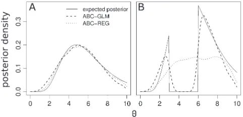
the simulated parameters, which makes estimation of the marginal posteriors of individual parameters particularly easy. The method can also be extended to more complex, nonlinear models as demonstrated, e.g., in Blum and Francois(2009). In extreme situations, however, ABC– REG may yield posteriors that are nonzero in parameter regions where the priors actually vanish (see Figure 1B for an illustration of this phenomenon). Moreover, it is not clear how ABC–REG could yield an estimate of the marginal density of modelMatsobs, information that is useful for model comparison.

In contrast to ABC–REG we treat the parametersuas exogenous and the summary statisticssas endogenous variables and we stipulate forMeðsobsÞa general linear model (GLM in the literature—not to be confused with the generalized linear models that unfortunately share the same abbreviation). To be precise, we assume the summary statisticss created by the truncated model’s likelihoodfeðsjuÞto satisfy

sju¼Cu1c01e; ð4Þ

whereCis an3mmatrix of constants,c0ann31 vector, and e a random vector with a multivariate normal distribution of zero mean and covariance matrixSs:

e N ð0;SsÞ:

A GLM has the advantage of taking into account not only the (local) linearity, but also the strong correlation normally present between the components of the summary statistics. Of course, the model assumption (4) can never represent the full truth since its statistics are in principle unbounded whereas the likelihood feðsjuÞis supported on thee-ball aroundsobs. But since the multivariate Gaussians will fall off rapidly in practice and not reach far out off the boundary ofBeðsobsÞ, this is a disadvantage we can live with. In particular, the ordinary least squares (OLS) estimate outlined below implies that for e/0 the constant c0 tends to sobs whereas the design matrixCand the covariance matrix

Ss both vanish. This means that in the limit of zero

tolerance e¼0 our model assumption yields the true posterior distribution ofM.

THEORY

In this section we describe the above methodology— referred to as ABC–GLM in the following—in more detail. The basic two-step procedure of ABC–GLM may be summarized as follows.

GLM1:Given a modelMcreating summary statisticss and given a value of observed summary statistics sobs, create a sample of retained parametersuj_;

j¼1;. . .;N, with the aid of some ABC sampler (rejection sampling, ABC–MCMC, or ABC–PRC) based on a prior distribution

GLM2: Estimate the truncated model MeðsobsÞ as a general linear model and determine, on the basis of the sampleuj

, from the truncated priorpeðuÞan approxima-tion to the posteriorpðujsobsÞaccording to Equation 3.

Let us look more closely at these two steps.

GLM1: ABC sampling:We refer the reader to Marjoram

et al. (2003) and Sisson et al. (2007) for details

con-cerning ABC algorithms and to Marjoramand Tavare´ (2006) for a comprehensive review of computational methods for genetic data analysis. In practice, the di-mension of the summary statistics is often reduced by a principal components analysis (PCA). PCA also has a certain decorrelation effect. A more sophisticated method of reducing the dimension of summary statis-tics, based on partial least squares (PLS), is described in Wegmannet al.(2009). In a recent preprint, Voglet al. (C. Vogl, C. Futschik and C. Schloetterer, un-published data) propose a Box–Cox-type transforma-tion of the summary statistics that makes the likelihood close to multivariate Gaussian. This transformation might be especially efficient in our context as we assume normality of the error terms in our model assumption. To fix the notation, letP ¼ fu1_{;. . .;u}N_{gbe a sample}

of vector-valued parameters created by some ABC algorithm simulating from some prior pðuÞ and S ¼ fs1_{; . . .;s}N_{g be the sample of associated summary}

statistics produced by the model M. Each parameter

uj_{is anm-dimensional column vectoru}j _{¼ ðu}j_{;. . .;u}j mÞ

t

and each summary statistic is ann-dimensional column vectorsj _{¼ ðs}j

1;. . . ;sjnÞ t _{2 Beð}

sobsÞ. The samplesP and

Scan thus be viewed asm3Nandn3NmatricesPand S, respectively.

The empirical estimate of the truncated priorpeðuÞis given by the discrete distribution that puts a point mass

of 1/N on each value uj _{2 P}

. We smooth out this empirical distribution by placing a sharp Gaussian peak over each parameter valueuj

. More precisely, we set

peðuÞ ¼

1 N

XN

j¼1

fðuuj;SuÞ; ð5Þ

where

fðuuj;SuÞ ¼

1

j2pSuj1=2

eð1=2ÞðuujÞtSu1ðuu j_Þ

and

Su¼diagðs1;. . .;smÞ

is the covariance matrix offthat determines the width of the Gaussian peaks. The larger the number N of sampled parameter values is, the sharper the peaks can be chosen to still get a rather smooth pe. If the

parameter domainPis normalized to [0, 1]m

, say, then a reasonable choice iss_k¼1/N. Otherwise,s_kshould be adapted to the parameter range of the parameter component uk. Too small values of sk will result in

wiggly posterior curves, and too large values might unduly smear out the curves. The best advice is to run the calculations with several choices for Su. If pe

induces a correlation between parameters, a nondiag-onalSumight be beneficial. In practice, however, the

posterior estimates are most sensitive to the diagonal values ofSu.

GLM2: general linear model: As explained in the

Introduction, we assume the truncated model

MeðsobsÞto be normal linear;i.e., the random vectors ssatisfy (4). The covariance matrixSsencapsulates the

Figure 1.—Comparison

of rejection (A and D), ABC–REG (B and E), and ABC–GLM (C and F) poste-riors with those obtained from analytical likelihood calculations. We estimated the population–mutation parameter u ¼ 4Nm of a panmictic population for different observed num-bers of segregating sites (see text). Shades indicate the L1 distance between the inferred and the analyt-ically calculated posterior. White corresponds to an exact match (zero distance) and darker gray shades in-dicate larger distances. If the inferred posterior dif-fers from the analytical more than the prior does, squares are marked in black. The top row (A–C) corresponds to cases with a uniform prior u

strong correlations normally present between the components of the summary statistics.C, c0, and Ss

can be estimated by standard multivariate regression analysis (OLS) from the sample P,S created in step GLM1. [Strictly speaking, one must redo an ABC sample from uniform priors overPto get an unbiased estimate of the GLM if the priorpðuÞis not uniform already. On the other hand, ordinary least-squares estimators are quite insensitive to the prior’s influence. In practice, one can as well use the samplePto do the estimate. We applied both estimation methods to the toy models presented in theexamples from popula-tion genetics section and found no significant difference between the estimated posteriors. The same holds true for the so-called feasible generalized least-squares (FGLS) estimator; see Greene(2003). In this two-stage algorithm the covariance matrix is first estimated as in our setting but in a second round the design matrixC is newly estimated. When we applied FGLS to our toy models, we found a difference in the estimated matrices only after the eighth significant decimal. FGLS is a more efficient estimator only when the sample sizes are relatively small as is often the case in economical data sets but not in ABC situations. In theory, both OLS and FGLS are consistent estimators but FGLS is more efficient.] To be specific, set X ¼

(1...Pt

), where 1is anN3 1 vector of 1’s.C andc0are determined by the usual least-squares estimator

ðˆc0.. .

ˆ

CÞ ¼SXðXt_XÞ1_;

and forSs we have the estimate

ˆ

S_s¼ 1

N mRˆ

t_ˆ

R; ð6Þ

whereRˆ ¼St_{X ðˆc}

0..

.

ˆ

CÞt are the residuals. The likeli-hood for this model—dropping the hats on the matrices to unburden the notation—is given by

feðsjuÞ ¼ j2pSsj1=2eð1=2ÞðsCuc0Þ

t_S1

s ðsCuc0Þ_{: ð7Þ}

An exhaustive treatment of linear models in a Bayesian (econometric) context is given in Zellner’s book (Zellner1971).

Recall from (3) that for a priorpðuÞand an observed summary statisticsobs, the parameter’s posterior distri-bution for our full modelMis given by

pðujsobsÞ ¼cfeðsobsjuÞpeðuÞ; ð8Þ

wherefeðsobsjuÞis the likelihood of the truncated model

MeðsobsÞgiven by (7) andpeðuÞis the estimated (and smoothed) truncated prior given by (5).

Performing some matrix algebra (see appendix a), one can show that the posterior (8) is—up to a

multiplicative constant—of the formPN_i¼jexpð1 2QjÞ,

where

Qj¼ ðutjÞtT1ðutjÞ1 . . .

. . . 1ðsobsc0ÞtS1_s ðsobsc0Þ1 . . . . . . 1ðuj_Þt_S1

u uj ðvjÞtTvj:

HereT,tj , andvj

are given by

T¼ ðCtS1_s C1S1u Þ1 ð9Þ

andtj_¼ Tvj

, where

vj¼CtS1_s ðsobsc0Þ1S1u uj: ð10Þ

From this we get

pðujsobsÞ} XN

j¼1

cðujÞeð1=2ÞðutjÞtT1ðutjÞ; ð11Þ

where

cðuj_{Þ ¼exp} 1

2ððu

j_Þt_S1

u uj ðvjÞtTvjÞ

: ð12Þ

When the number of parameters exceeds two, graph-ical visualization of the posterior distribution becomes impractical and marginal distributions must be calcu-lated. The marginal posterior density of the parameter

u_kis defined by

pðukjsÞ ¼ ð

Rm1

pðujsÞduk;

where integration is performed along all parameters exceptuk.

Recall that the marginal distribution of a multivariate normalN ðm;SÞwith respect to thekth component is the univariate normal density N ðm_k;sk;kÞ. Using this

fact, it is not hard to show that the marginal posterior of parameterukis given by

pðukjsobsÞ ¼a XN

j¼1

cðujÞexp ðukt j kÞ2

2t_k;k !

; ð13Þ

wheret_k,kis thekth diagonal element of the matrixT,tkj

is the kth component of the vector tj_{, and}

cðuj_{Þis still}

large values ofNthe diagonal elements in the matrixSu

can be chosen so small that the error is in any case negligible.

Model selection: The principal difficulty of model selection methods in nonparametric settings is that it is nearly impossible to estimate the likelihood ofMatsobs due to the high dimension of the summary statistics (curse of dimensionality); see Beaumont(2007) for an approach based on multinomial logit. Parametric mod-els on the other hand lend themselves readily to model selection via Bayes factors. Given the model M, one must determine the marginal density

fMðsobsÞ ¼ ð

P

fðsobsjuÞpðuÞdu:

It is easy to check from (1) and (2) that

fMðsobsÞ ¼Aeðsobs;pÞ ð

P

feðsobsjuÞpeðuÞdu:

Here

Aeðsobs;pÞ:¼ ð

P

pðuÞ ð

Be

fMðsjuÞdsdu ð14Þ

is the acceptance ratepof the rejection process. It can easily be estimated with aid of ABC–REJ: Sample parameters from the priorpðuÞcreate the correspond-ing statisticssfromMand count what fraction of the statistics fall into thee-ballBecentered atsobs.

If we assume the underlying model ofMeðsobsÞto be our GLM, then the marginal density ofMatsobscan be estimated as

fMðsobsÞ ¼

Aeðsobs;pÞ

N j2pDj1=2 XN

j¼1

eð1=2ÞðsobsmjÞtD1ðsobsmjÞ_;

ð15Þ

where the sum runs over the parameter sample

P ¼ fu1_{;. . .;u}N_g,

D¼Ss1CSuCt

and

mj¼c01Cuj:

For two modelsMAandMB with prior probabilities

p_A andp_B ¼1 – p_A, the Bayes factor BAB in favor of

modelMAover modelMB is

BAB¼

fMAðsobsÞ fMBðsobsÞ

; ð16Þ

where the marginal densitiesfMAandfMBare calculated according to (15). The posterior probability of model

MAis

fðMAjsobsÞ ¼

BABpA

BABpA1pB

:

EXAMPLES FROM POPULATION GENETICS

Toy models:In Figure 1 we present the comparison of posteriors obtained with rejection sampling, ABC–REG and ABC–GLM, with those determined analytically (‘‘true posteriors’’). As a toy model we inferred the population–mutation parameteru¼4Nmof a panmictic population model from the number of segregating sites Sof a sample of sequences with 10,000 bp for different observed values and tolerance levels. Estimations are always based on 5000 simulations with dist(S,Sobs),e, and we report the average of 25 independent replica-tions per data point. Estimation bias of the different approaches was assessed by computing the total varia-tion distance between the inferred posterior and the true one obtained from analytical calculations using the likelihood function introduced by Watterson(1975). Recall that theL1-distance of two densitiesf(u) andg(u) is given by

d1ðf;gÞ ¼

1 2

ð

jfðuÞ gðuÞjdu:

It is equal to 1 whenfandghave disjoint supports and it vanishes when the functions are identical.

When we used a uniform prioruUnif([0.005, 10]) (Figure 1, A–C), both ABC–REG and ABC–GLM give comparable results and improve the posterior estima-tion compared to the simple rejecestima-tion algorithm except for very low tolerance values e where the rejection algorithm is expected to be very close to the true posterior. The average total variation distances over all observed data sets and tolerance values e are 0.236, 0.130, and 0.091 for the rejection algorithm, ABC–REG, and ABC–GLM, respectively. Note that perfect matches between the approximate and the true posteriors are difficult to obtain because all approximate posteriors depend on a smoothing step that may not give accurate results close to borders of their supports. However, when we used a discontinuous prioruUnif([0.005, 3][[6, 10]) with an admittedly extremely artificial ‘‘gap’’ in the middle, we observed a quite distinct pattern (Figure 1, D and E). One clearly recognizes that posteriors inferred with ABC–REG are frequently misplaced and often even farther away from the true posterior (in total variation distance) than the prior, especially for cases where the likelihood of the observed data is maximal within the gap. The reason for this is that in the regression step of ABC–REG parameter values may easily be shifted out-side the prior support. This behavior of ABC–REG has been observed earlier (Beaumont et al.2002; Estoup

Hamilton et al. (2006) proposed to transform the parameter values prior to the regression step by a transformation of the form y¼ lnðtanðððxaÞ=

ðbaÞÞðp=2ÞÞ1Þ, where a and b are the lower and upper borders of the prior support interval. For more complex priors—like the discontinuous prior used here—this transformation may not work. ABC–GLM is much less affected by the gap prior than ABC–REG. The average total variation distances over all observed data sets and tolerance valueseare 0.221, 0.246, and 0.094 for the rejection algorithm, ABC–REG, and ABC–GLM, respectively. Example posteriors withSobs¼16 based on 5000 simulations with dist(S,Sobs), 10 are shown in Figure 2.

The success of ABC–GLM depends on how well a general linear model fits the truncated modelMeðsobsÞ. Under the null hypothesis that the fit is perfect the estimated residuals rj (see Equation 6) are

indepen-dently multivariate normally distributed random vec-tors. Hence the Mahalanobis distances

dj¼rtjS 1

s rjx2n ð17Þ

follow ax2_{-distribution withndegrees of freedom. As a}

quantification of model assessment we propose to report the Kolmogorov–Smirnov test statistic for the empirical distribution ofdjand the reference x2

-distri-bution. (Reporting P-values will be of little use in practice since the null hypothesis does never hold exactly and hence theP-values will become very small due to the large sample size.)

When the summary statistics are created from a general linear model, the fit should be optimal. This is indeed the case as the simulation results in Table 1 show. We performed 200 simulations of randomly created general linear models withm ¼ 3 parameters, n ¼4 summary statistics, and a multivariate normal prior. The observed statistics were also created from the respective models. For each simulated observed statistic and

different acceptance rates p ¼ 1.00, 0.50, 0.10, 0.05, and 0.01 we calculated the approximate posterior distributions pe, pREG, and pGLM for the rejection algorithm, ABC–REG, and ABC–GLM, respectively. As the prior is multivariate normal, the true posteriorp0 can be analytically determined. Table 1 contains the means and standard deviations over the 200 simulations of the total variation distances of the approximate posteriors to the true posteriorp0as well as the mean and standard deviations of the Kolmogorov–Smirnov test statistics for the GLM model fit. As is expected, the model fit is perfect [i.e., the Kolmogorov–Smirnov (KS) statistic is close to 0] for acceptance ratep¼1. As the acceptance rate becomes lower, the model fit deterio-rates since the truncated model of a GLM is no longer exactly a general linear model. The total variation distance to the true posterior increases slightly aspgets smaller but the improved rejection posteriorpemostly

outbalances the poorer model fit. As is expected in this ideal situation, ABC–GLM and ABC–REG substantially improve the posterior estimation over the pure re-jection prior.

To test the other extreme we performed 200 simu-lations for a nonlinear one-parameter model with uniformly rather than normally distributed error terms; the prior was again a normal distribution. (The details of this toy model are described inappendix b.) As Table 2 shows, the GLM model fit is already poor for an acceptance rate of p ¼ 1.00 (KS statistic 0.10) and further deteriorates as p decreases. Note that the approximate posteriors pREG and pGLM are closer to the true posterior in average than pe and that both

adjustment methods perform similarly. As expected, the accuracy of the posteriors increases with smaller accep-tance rates, despite the fact that the model fit within the

e-ball decreases. This suggests that the rejection step contributes substantially to the estimation accuracy, especially when the true model is nonlinear. We should mention that in30% of the simulations both ABC– GLM and ABC–REG actually increased the distance to the true posterior in comparison to the rejection posteriorpe. As a rule of thumb we suggest that posterior Figure _{2.—Example posteriors for uniform (A) and}

dis-continuous (B) priors. The model is the same as in Figure 1. Posterior estimates using ABC–GLM and ABC–REG for

Sobs¼16 were based on 5000 simulations with dist(S,Sobs), 10. ABC–REG posteriors were smoothed with a bandwidth of 0.4, and the width of the Dirac peaks in the ABC–GLM approach was set to 105_.

TABLE 1

Mean and standard deviation of theL1distance between inferred and expected posteriors for randomly generated GLMs withNP¼3,NS¼4 [priorN(0, 0.22), 200 simulations]

pa _d

1(p0,pe) d1(p0,pREG) d1(p0,pGLM) KS statisticsb 1.00 0.5160.22 0.1560.10 0.0160.001 0.00460.001 0.50 0.4260.19 0.1360.10 0.0260.008 0.00760.003 0.10 0.2960.18 0.1360.11 0.0360.01 0.0260.01 0.05 0.2460.16 0.1360.12 0.0360.01 0.0360.01 0.01 0.2160.17 0.1560.14 0.0560.02 0.0660.02

a_{Acceptance rate as a fraction.}

adjustments obtained by ABC–GLM or ABC–REG should not be trusted without further validation if the Kolmogorov–Smirnov statistic for the GLM model fit exceeds a value of, say, 0.10. In that case linear models are not sufficiently flexible to account for effects like nonlinearity in the parameters and nonnormality and heteroscedasticity in the error terms. In the setting of ABC–REG a wider class of models is introduced in Blum and Francois (2009), where machine-learning algo-rithms are applied for the parameter estimations. Whether these extensions can be applied in our context remains to be seen. The advantage of the general linear model is that estimations can be done with ordinary least squares and the important quantities like marginal posteriors and marginal likelihoods can be obtained analytically. For more complex models these quantities will probably be accessible only via numerical integra-tion, Monte Carlo methods, etc.

Application to chimpanzees:In standard taxonomies, chimpanzees, the closest living relatives of humans, are classified into two species: the common chimpanzee (Pan troglodytes) and the bonobo (P. paniscus). Both species are restricted to Africa and diverged 9 MYA (Wonand Hey2005; Becquetand Przeworski2007). The common chimpanzees are further subdivided into three large populations or subspecies on the basis of their separation by geographic barriers. Among them, the western chimpanzees (P. troglodytes verus) form the most remote group. Interestingly, recent multilocus studies found consistent levels of gene flow between the western and the central (P. t. troglodytes) chimpan-zees (Won and Hey 2005; Becquet and Przeworski 2007). Nonetheless, a recent study of 310 microsatellites in 84 common chimpanzees supports a clear distinction between the previously labeled populations (Becquet

et al. 2007). Using a PCA analysis, indication for

sub-structure within the western chimpanzees was found in the same study.

To demonstrate the applicability of the model selec-tion given in the theory section we contrast two different models of the western chimpanzee population

with this data set: a model of a single panmictic population with constant size and a finite island model of constant size and constant migration among demes. While we estimatedu¼2Nem, priors were set onNeand

m separately with log10(Ne) Unif([3, 5]) and m

N(53104_{, 2310}4_{) truncated onm2[10}4_{, 10}3_{]. In}

the case of the finite island model, we had an additional priornpopUnif([10, 100]) on the number of islands, and individuals were attributed randomly to the differ-ent islands.

We obtained genotypes for all 50 individuals reported to be of western chimpanzee origin from the study of Becquetet al.(2007), excluding captive-born hybrids. We checked the proposed (Becquet et al. 2007) mutation pattern for each individual locus, and all alleles not matching the assumed stepwise mutation model were set as missing data. A total of 265 loci were used, after removing the loci on the X and the Y chromosome as well as those being monomorphic among the western chimpanzees. All simulations were performed using the software SIMCOAL2 (Lavaland Excoffier 2004) and we reproduced the pattern of missing data observed in the data set. Using the software package Arlequin3.0 (Excoffieret al.2005), we calcu-lated two summary statistics on the data set: the average number of alleles per locus, K, and FIS, the fixation index within the western chimpanzees. We performed a total of 100,000 simulations per model.

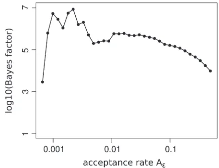
In Figure 3 we report the Bayes factor of the island model according to (16) for different acceptance rates Ae; see (14). While there is a large variation for very

small acceptance rates, the Bayes factor stabilizes for Ae$0.005. Note thatAe#0.005 corresponds to,500

simulations and that the ABC–GLM approach, based on a model estimation and a smoothing step, is expected to TABLE 2

Mean and standard deviation of theL1distance between inferred and expected posteriors for the uniform errors

model (seeAPPENDIX B) withNP¼1,NS¼5 {prior

N(0, 22_{), error Unif[10, 10], 200 simulations}}

pa _d

1(p0,pe) d1(p0,pREG) d1(p0,pGLM) KS statisticsb 1.00 0.5660.24 0.4960.25 0.4660.29 0.0960.01 0.50 0.4060.30 0.3660.28 0.3760.27 0.1260.01 0.10 0.3860.28 0.3560.26 0.3460.23 0.1460.03 0.05 0.3460.29 0.3360.27 0.3260.23 0.1460.02 0.01 0.2960.23 0.2660.22 0.2660.18 0.1660.03

a

Acceptance rate as a fraction.

b_{KS statistic describing the linear model fit (see text).}

Figure3.—Bayes factor for the island relative to the

pan-mictic population model for different acceptance rates (log-arithmic scale). For very low acceptance rates we observe large fluctuations whereas the Bayes factor is quite stable for larger values. Note thatAe#0.005 corresponds to#500 simulations,

produce poor results since the estimation of the model parameters is unreliable due to the small sample size. The good news is that the Bayes factor is stable over a large range of tolerance values. We may therefore safely reject the panmictic population model in favor of population subdivision among western chimpanzees with a Bayes factor ofB105_.

DISCUSSION

Due to still increasing computational power it is nowadays possible to tackle estimation problems in a Bayesian framework for which analytical calculation of the likelihood is inhibited. In such cases, approximate Bayesian computation is often the choice. A key innovation in speeding up such algorithms was the use of a regression adjustment, termed ABC–REG in this article, which used the frequently present linear relationship between generated summary statistics s and parameters of the modeluin a neighborhood of the observed summary statisticssobs(Beaumontet al. 2002). The main advantage is that larger tolerance valuesestill allow us to extract reasonable information about the posterior distributionpðujsÞand hence less simulations are required to estimate the posterior density.

Here we present a new approach to estimate approx-imate posterior distributions, termed ABC–GLM, simi-lar in spirit to ABC–REG, but with two major advantages: First, by using a GLM to estimate the likelihood function, ABC–GLM is always consistent with the prior distribution. Second, while we do not find the ABC– GLM approach to substantially outperform ABC–REG in standard situations, it is naturally embedded into a standard Bayesian framework, which in turn allows the application of well-known Bayesian methodologies such as model averaging or model selection via Bayes factors. Our simulations show that the rejection step is especially beneficial if the true model is nonlinear for both ABC approaches. ABC–GLM is further compatible with any type of ABC sampler, including likelihood-free MCMC (Marjoram et al. 2003) or population Monte Carlo (Beaumont et al. 2009). Also, more complicated re-gression regimes taking nonlinearity or heteroscedacity into account may be envisioned when the GLM is replaced by some more complex model. A great advantage of the current GLM setting is its simplicity, which renders implementation in standard statistical packages feasible.

We showed the applicability of the model selection procedure via Bayes factors by opposing two different models of population structure among the western chimpanzees P. troglodytes verus. Our analysis strongly suggests population substructure within the western chimpanzees since an island model is significantly favored over a model of a panmictic population. While

none of our simple models is thought to mimic the real setting exactly, we still believe that they capture the main characteristics of the demographic history influencing our summary statistics, namely the number of alleles Kand the fixation indexFIS. While the observedFISof 2.6% has been attributed to inbreeding previously (Becquet et al. 2007), we propose that such values may easily arise if diploid individuals are sampled in a randomly scattered way over a large, substructured population. While it was almost impossible to simulate the value FIS ¼ 2.6% in the model of a panmictic population, it easily falls within the range of values obtained from an island model.

We are grateful to Laurent Excoffier, David J. Balding, Christian P. Robert, and the anonymous referees for their useful comments on a first draft of this manuscript. This work has been supported by grant no. 3100A0-112072 from the Swiss National Foundation to Laurent Excoffier.

LITERATURE CITED

Beaumont, M., 2007 _{Simulations, Genetics, and Human Prehistory—A} Focus on Islands.McDonald Institute Monographs, University of Cambridge, Cambridge, UK.

Beaumont_{, M., W. Z}hang _{and D. B}alding_{, 2002 Approximate}

Bayesian computation in population genetics. Genetics 162: 2025–2035.

Beaumont, M., R. C. Cornuetand J.-M. Marin, 2009 Adaptive

ap-proximate Bayesian computation. Biometrika (in press). Becquet, C., and M. Przeworski, 2007 A new approach to estimate

parameters of speciation models with application to apes. Genome Res.17:1505–1519.

Becquet, C., N. Patterson, A. Stone, M. Przeworskiand D. Reich,

2007 Genetic structure of chimpanzee populations. Genome Res.17:1505–1519.

Blum_{, M., and O. F}rancois_{, 2009 Non-linear regression models}

for approximate Bayesian computation. Stat. Comput. (in press).

Estoup, A., M. Beaumont, F. Sennedot, C. Moritz and J. M.

Cornuet_{, 2004 Genetic analysis of complex demographic}

sce-narios: spatially expanding populations of the cane toad, Bufo marinus. Evolution58:2021–2036.

Excoffier_{, L., G. L}aval_{and S. S}chneider_{, 2005 Arlequin (version}

3.0): an integrated software package for population genetics data analysis. Evol. Bioinform. Online1:47–50.

Greene, W., 2003 Econometric Analysis, Ed. 5. Pearson Education,

Upper Saddle River, NJ.

Hamilton, G., M. Stonekingand L. Excoffier, 2006 Molecular

analysis reveals tighter social regulation of immigration in patri-local populations than in matripatri-local populations. Proc. Natl. Acad. Sci. USA102:7476–7480.

Laval, G., and L. Excoffier, 2004 Simcoal 2.0: a program to

sim-ulate genomic diversity over large recombining regions in a sub-divided population with a complex history. Bioinformatics20: 2485–2487.

Lindley_{, D., and A. S}mith_{, 1972 Bayes estimates for the linear}

model. J. R. Stat. Soc. B34:1–44.

Marjoram_{, P., and S. T}avare´_{, 2006 Modern computational}

ap-proaches for analysing molecular genetic variation data. Nat. Rev. Genet.10:759–770.

Marjoram, P., J. Molitor, V. Plagnoland S. Tavare´_{, 2003 Markov}

chain Monte Carlo without likelihoods. Proc. Natl. Acad. Sci. USA100:15324–15328.

Sisson, S., Y. Fanand M. Tanaka, 2007 Sequential Monte Carlo

without likelihoods. Proc. Natl. Acad. Sci. USA104:1760–1765. Tallmon, D. A., G. Luikartand M. A. Beaumont, 2004

Tavare´, S., D. Balding, R. Griffithsand P. Donnelly, 1997

In-ferring coalescence times from DNA sequence data. Genetics 145:505–518.

Watterson_{, G., 1975 Number of segregating sites in genetic}

mod-els without recombination. Theor. Popul. Biol.7:256–276. Wegmann_{, D., C. L}euenberger_{and L. E}xcoffier_{, 2009 Efficient}

approximate Bayesian computation coupled Markov chain Monte Carlo without likelihood. Genetics182:1207–1218. Weiss_{, G., and A.}von_Haeseler_{, 1998 Inference of population}

his-tory using a likelihood approach. Genetics149:1539–1546.

Won, Y., and J. Hey, 2005 Divergence population genetics of

chim-panzees. Mol. Biol. Evol.22:297–307.

Zellner, A., 1971 An Introduction to Bayesian Inference in Econometrics.

Wiley, New York.

Communicating editor: J. Wakeley

APPENDIX A: PROOFS OF THE MAIN FORMULAS

To keep this article self-contained, we present a proof of formulas (11) and (15). The argument is an adaptation from the proof of Lemma 1 in Lindleyand Smith(1972). By linearity it clearly suffices to show the formulas for one fixed sampled parameteruj

. The results then follow.

Theorem.Suppose that, given the parameter vectoru,the distribution of the statistics vectorsis multivariate normal,

s N ðCu1c0;SsÞ;

and,given the fixed parameter vectoruj_{,the distribution of the parameteruis}

u N ðuj_;S

uÞ:

Then:

1.The distribution ofugivensis

ujs N ðTvj;TÞ;

whereT¼ Ct_S1

s C1S

1

u

1

andvj _¼Ct_S1

s ðsc0Þ1S

1

u u

j_.

2.The marginal distribution ofsis

s N ðmj;DÞ;

wheremj_¼c

01Cuj andD¼Ss1CSuCt.

Proof. By Bayes’ theorem

pðujsÞ}fðsjuÞpðuÞ:

The product on the right-hand side is of the form expð1

2QÞ, where

Q ¼ ðsc0CuÞtS1s ðsc0CuÞ1ðuujÞtS1u ðuujÞ

¼ut_ðCt_S1 s C1S

1

u Þu2ððsc0ÞtS1s Cu1ðujÞtS 1

u Þu1 . . .

. . . 1ðsc0ÞtS1s ðsc0Þ1ðujÞtS1u uj

¼utT1u2ðvjÞt_u1ðsc

0ÞtS1s ðsc0Þ1ðujÞtS1u uj

¼ ðuTvj_Þt_T1_ðuTvj_{Þ ðv}j_Þt_Tvj_{1 . . .} . . . 1ðuj_Þt_S1

u uj1ðsc0ÞtS1s ðsc0Þ:

In the last step we completed the square with respect touand used the fact thatTis symmetric. Up to a constant that does not depend onuj _{we hence get}

pðujsÞ}cðuj_Þexp 1

2ððuTv

j_Þt_T1_ðuTvj_ÞÞ

;

where cðuj_{Þ ¼}

expð1 2ððu

j_Þt

Su1u

j _ð

vj_Þt

Tvj_{ÞÞ. This proves the first part of the theorem and—by linear}

To prove the second part of the theorem, observe that s¼Cu1c01e with e N ð0;SsÞ and u¼uj1h with

h N ð0;SuÞ. Putting these equalities together, we get

sCuj_1c

01Ch1e:

This, being a linear combination of independent multivariate normal variables, is still multivariate normal with mean Cuj_1c

0and its covariance matrix is given by

E½ðCh1eÞðCh1eÞt _{¼E½ChðChÞ}t_1eet _¼CE½hht_Ct_1E½eet _¼CS

uCt1Ss:

This proves the second part of the theorem as well as formula (15). n

APPENDIX B: NONLINEAR TOY MODELS

In this section we describe a class of toy models that are nonlinear in the parameteru2R_{and have nonnormal,} possibly heteroscedastic error terms. Still their likelihoods are easy to calculate analytically. We set

s¼fðuÞ1eðuÞ ¼

f1ðuÞ .. .

fnðuÞ 0 B @

1 C A1

e₁ðuÞ .. .

e_nðuÞ 0 B @

1 C A:

Herefi(u) are monotonically increasing continuous functions ofuandei(u) are independent, uniformly distributed

error terms in the interval [–ui(u),ui(u)]4R, whereui(u) are nondecreasing, continuous functions:

e_iðuÞ Unifð½uiðuÞ;uiðuÞÞ:

It is straightforward to check that for a priorp(u) the posterior distribution ofugivens¼ ðs1;. . . ;snÞ t

is (up to a normalizing constant)

pðujsÞ} 1

u1ðuÞ . . .unðuÞ

Indð½u_min;u_maxÞpðuÞ;

where

u_min¼max i

fg_i1ðsiÞg; umax¼min

i

fh1_i ðsiÞg

and

giðuÞ ¼fiðuÞ1uiðuÞ; hiðuÞ ¼fiðuÞ uiðuÞ:

For the simulations in Table 2 we chosen¼5,f1ðuÞ ¼ ¼f5ðuÞ ¼u3_{, and}

u1ðuÞ ¼ ¼u5ðuÞ[10. The prior was