Learning Place Cells from Sonar Data
R.B. Ollington
School of Computing
University of Tasmania
Sandy Bay, Tasmania, Australia
[email protected]
P. W. Vamplew
School of Computing
University of Tasmania
Sandy Bay, Tasmania, Australia
[email protected]
A
BSTRACTA place cell system is developed that is able to provide robust localisation using simple sonar information only. The system uses egocentric view cells, based on the Adaptive Response Function Neuron, as sensory input to correct for path integration errors. The major advantage of this system is that place field centres are fixed prior to training, allowing downstream navigational systems to make relevant predictions immediately upon entering a new environment.
1. INTRODUCTION
Tolman [1] proposed that the brain might hold a topological map of its environment and that this map could be used for various navigational tasks. Studies of brain lesions in animals and humans have identified the hippocampus as a possible location for spatial cognition. O’Keefe and Dostrovsky [2] observed that certain cells in the hippocampus of rats responded maximally when the rat was in a certain location. O’Keefe and Nadel [3] suggested that these cells might form the basis of a cognitive map. The cognitive map theory has also been strengthened by later experiments such as those involving the Morris Watermaze [4, 5].
Place cells, as these neurons are called, fire strongly only when the head of the rat is within the cells “place field” and in many cases this field is independent of the activity being performed or the direction the rat is facing. Place cells generally have only one place field within a particular environment. Place fields in different environments are not correlated, and a cell exhibiting a place field in one environment may have no place field in another [6].
Place fields are influenced by visual stimulus. If visible landmarks within an environment are rotated then place fields rotate with respect to each other by the same amount [6, 7]. However, in the absence of visual stimulus, place cells persist [6-8] and hence idiothetic information, such as vestibular, visual motion and motor afferent inputs, must also be able to influence place cell firing. Other experiments also confirm that path-integration or dead-reckoning is a crucial component of navigation in many animals [9, 10].
Several navigational models based on place cells have been developed [11, 12]. These models clearly
demonstrate the value of place cells for artificial and biological navigation. Computational models for the formation of place cells have also been developed. However, many of these methods work only in simplified or stylised environments [13, 14].
A system was developed for training place cells using simple sonar input. The main advantage of the new system is that place field centres are set independently of the environment. Knowing the relative positions of place fields prior to entering the environment will improve performance of navigational systems in the early stages of exploration.
The system first trains view cells to recognise particular sensory input patterns. These view cells provide a degree of positional discrimination that is then refined by path integration input to produce place cells. View cells are discussed in section 2, while the place cell system is discussed in section 3.
2. VIEW CELLS
View cells should be able to accurately capture the salient information of the view at a particular location and orientation. While substantial changes in that position and orientation should result in a significantly decreased firing of the view cell, minor changes should not result in a major change. Many researchers have found a simple gaussian function sufficient to model view cells. However these experiments take place in simple environments, and/or it is assumed that the view cell input has already been significantly processed (eg. by finding the orthogonal distance to walls).
Sonar 1 Distance Response Sonar 2 Distance Response 1 2
Figure 1: Left: A robot with two sonar faces a typical wall section. Right: Response functions that would be suitable to capture this view.
2.1. ADAPTIVE RESPONSE FUNCTION NEURONS
The ARFN [15] is a neural model capable of learning the centre, size and shape of a locally tuned response function. ARFNs compute the difference between two sigmoids for a given input. The thresholds and gains of each sigmoid are trained independently. Figure 2 shows example response functions for an ARFN trained to recognise category one of the iris data set [16].
0 2 4 6 8 10 12
0 0.1 0.2 0.3 0.4 0.5 0.6 0.7 0.8 0.9 1
Input 1 Frequency 0 0.2 0.4 0.6 0.8 1 Response Frequency Response Function 0 1 2 3 4 5 6 7 8 9 10
0 0.1 0.2 0.3 0.4 0.5 0.6 0.7 0.8 0.9 1
Input 2 Frequency 0 0.2 0.4 0.6 0.8 1 Response Frequency Response Function 0 5 10 15 20 25
0 0.1 0.2 0.3 0.4 0.5 0.6 0.7 0.8 0.9 1
Input 3 Fr equency 0 0.2 0.4 0.6 0.8 1 R e sponse Frequency Response Function 0 5 10 15 20 25 30
0 0.1 0.2 0.3 0.4 0.5 0.6 0.7 0.8 0.9 1
Input 4 Frequency 0 0.2 0.4 0.6 0.8 1 Response Frequency Response Function
Figure 2: The response functions learned for each input of an ARFN trained on category one of the iris data set. Also shown is the frequency distribution of the data set (dotted line).
2.2. ARFNS AS VIEW CELLS
To test the viability of ARFNs as view cells a simulated robot was used to train 256 view cells, arranged in a 16×16 array, while undergoing a collision avoidance task in the simple environment shown in Figure 5. The robot had 9 sonar sensors at angles of –135, -90, -45, -22.5, 0, 22.5, 45, 90, and 135 degrees with respect to the orientation of the robot.
For the view system, ARFN view cells are trained using a simple self-organising map algorithm, with some modifications to the standard procedure. To encourage rapid early learning and long-term stability, each cell maintains a training rate modifier. This modifier is reduced when the cell is the “winning” cell for a given input, and increased otherwise as shown below:
mod if mod mod otherwise i i i i w α β × = = + (1)
where w is the index of the winning cell, 0<α<1 and b is some small value.
Cells that are rarely identified as the winning cell will have a higher training rate than cells which are frequent winners. The effective training rate for a cell iis:
(
) (
2)
22
exp
rate mod w i w i
i i x x y y
σ
− + −
= ×
(2)
where xw,yw are the SOM coordinates of the winning
neuron, xi,yi are the SOM coordinates of cell i, and σ is
the neighbourhood size. This rate defines the extent to which each ARFN is trained [15]
Cell 16
0 3
6 Cell 20
0 3 6 Cell 76 0 3
6 Cell 80
0 3 6 Cell 24 0 3
6 Cell 28
0 3 6 Cell 84 0 3
6 Cell 88
0 3 6 Cell 136 0 3
6 Cell 140
0 3 6 Cell 196 0 3
6 Cell 200
0 3 6 Cell 144 0 3
6 Cell 148
0 3 6 Cell 204 0 3
6 Cell 208
0 3 6
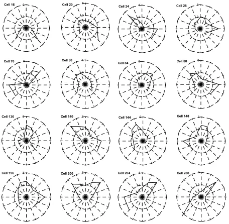
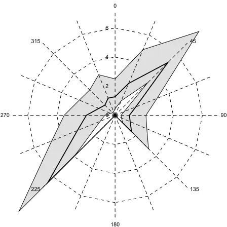
[image:2.612.63.283.325.661.2] [image:2.612.326.554.446.669.2]Figure 3 shows the views learnt by 16 of these cells, while Figure 4 shows a detailed plot of the response function learned for cell 208. Cell 208 has learned a view where the robot is moving obliquely across a narrow space running from left rear to forward right. Note that the width of the space is well defined (narrow response function), whereas the length is less well defined (broad response function). The minimum distances of walls are also more tightly constrained than the maximum distances. This cell will recognise a corridor-like area at a particular orientation.
0 2 4 6 0
45
90
135
180 225
270 315
Figure 4: Sonar response function learned by cell 208. The thick line plots the range at which each input fires maximally, while the shaded region shows the ranges at which each input response is over 0.75.
ARFN view cells are able to detect a range of situations with similar salient features. Without the ability to learn variable response function widths, the view cells would be much more limited. For example, in the corridor situation above, a view cell with a fixed narrow response function would identify corridors of one particular length. In contrast, a view cell with a broad response function would respond to open spaces as well as corridors.
The usefulness of these view cells for localisation is clearly illustrated in Figure 5. The place fields of cell 24 are elongated and follow the topology of the environment. While initially this may seem problematic, it is interesting to note that many biological place fields also have this property. Although place fields such as this may cause some problems for place cells and hence navigation, they should assist in the generalisation ability of the system in other areas. For example, if these view cells were the input for a collision avoidance system these place fields would be ideal, since the optimal action is likely to be very similar for the entire length of the field. The overlapping place fields of other cells,
such as cell 196, should help reduce ambiguity where a more restricted place code is required.
Cell 24
Cell 196
[image:3.612.327.547.84.269.2]Cell 208
[image:3.612.59.283.186.410.2]Figure 5: Location and orientation where the winning ARFN was either cell 24, 196 or 208. Solid lines represent walls. Dotted ovals show groups of cells sampled at similar orientations, with the average orientations indicated by arrows.
Figure 5 shows the locations and orientations where each of three selected cells was the most active in the SOM. For any given orientation, these view cells may have more than one place field. However, these fields are generally sufficiently separated that they should be distinguishable through path integration, with the possible exception of cell 24.
3. FROM VIEW CELLS TO PLACE CELLS
The view cells produced by the system described in the previous section provide a good basis for place cell input. View cells show good place and orientation discrimination however they often have place fields in more than one position and orientation. If a good estimate of head direction is available then this situation is significantly improved. A path integration system that allows only those places that are within a reasonable distance of the current estimate to be recognised would be sufficient to resolve any remaining ambiguity. This section presents a method for combining view cell and path integration input and for using the resultant place cells to update the position estimate.
3.1. COMBINING PATH INTEGRATOR AND VIEW CELL
INPUT
Each place cell is assigned a fixed set of path integrator coordinates. Any method may be chosen, but for the current work, the assigned coordinates correspond to a square grid of place field centres. This assignment is made with no knowledge of the environment other than the maximum size. Path integrator coordinates are primarily updated from odometric estimates of the change in position. The primary influence on place cell activity is based on the gaussian distance of the centre of the cell’s place field from the current path integrator coordinates. The path integrator contribution to the activation of place cell i is given by:
2
2
exp 2
i i
p s PI
σ
− −
=
(3)
where
p
is the current path integration vector,s
i is the centre of place cell i’s place field and σ is a parameter controlling the range of the path integrator contribution.Odometric errors may result from undetectable occurrences such as wheel slip or collisions. These errors will cause cumulative path integration errors and must be corrected by view cell input. View cell input alone, however, should not be sufficient to cause place cell firing. Therefore, view cell input is used to moderate the path integrator input.
The place cell system learns an association between view cell input and place cell firing. However, view cell input may be significantly different for different robot headings in the same place and so the association is learned for a discrete set of orientations. During each update cycle the weight,
w
ijd, from view cell i to place cell j, for direction d is adjusted using:ˆ
(1 )( ) ,
0 ,
d j j i
ij
PC PC VC if d h
w
otherwise
η α
− − =
∆ =
(4)
where
h
ˆ
is the discretised value of the current heading,h; VCi is the output of view cell i; PCj is the output of
place cell j; α is a parameter determining the equilibrium position for weight changes; and η is the training rate. If the current heading is
h
ˆ
, the view cell input to place cellj is given by:
ˆ
1 0.5
1 exp ( )
j
h ij i i
VI
w VC α
= −
+ − −
∑
(5)
The final place cell output is given by:
(
1)
1 exp j
j j
PC
aPI bVI
t
=
+
+ −
(6)
where the parameters t, a and b are chosen so that view cell input alone does not produce significant place cell activation.
3.2. PLACE FIELDS
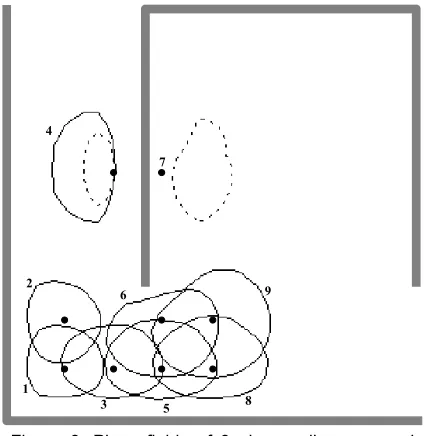
The place fields generated in this way should show a high degree of positional selectivity. The shapes of place fields will also be influenced by the current view and hence the orientation of the robot. Figure 6 shows place fields of nine place cells sampled during a collision avoidance task.
1
7
9
8 6
5 3 4
[image:4.612.333.545.149.367.2]2
Figure 6: Place fields of 9 place cells, averaged over all robot orientations. Small solid circles indicate Place field centres. Solid contours indicate an activation level of 0.5, and are shown for 9 cells (Cells 1-6,8,9). The dotted contours indicate the 0.25 activation level of a single bimodal place cell (Cell 7).
The generated place fields show a high degree of overlap, which would provide good generalisation for a navigational system based on these cells. The shapes of place fields also conform to the environment, potentially providing additional environmental information. A more detailed analysis of these fields follows in Figure 7.
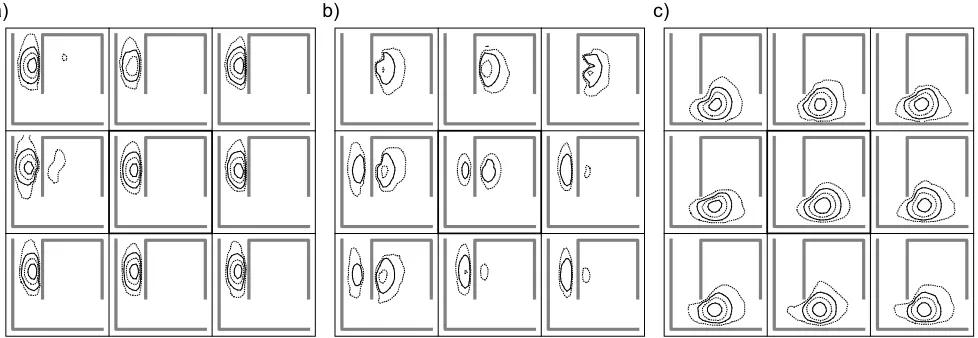
The field of cell 4 is elongated along the corridor and, since the appropriate action is not likely to change in this region, this should be a beneficial property. For orientations to the northwest and west, this cell shows some bimodal behaviour. However, the activity level in the secondary field is very low and not likely to affect navigation.
a) b) c)
Figure 7: Place field detail for cells 4(a), 7(b) and 9(c). Dotted contours indicate activation levels of 0.15 and 0.5, solid contours indicate activation levels of 0.3 and 0.7. The central panel of each figure shows the average activation over all robot headings, the surrounding panels show the activation average of headings within 22.5 degrees of each compass point.
Cell 7 has a place field with a distinctly bimodal nature. In addition, the area of greatest activity is dependent upon the orientation of the robot. Furthermore, the two centres of activity are located on opposite sides of the wall. This cell would not be suitable as input to a navigational system. However, the maximum output of this cell is considerably lower than for other cells and in fact the output of this cell was always dominated by neighbouring cells such as cell 4.
3.3. CORRECTING ODOMETRIC ERRORS
The place fields generated by this algorithm show many of the properties of biological place fields and should provide valuable input to the navigational system. In addition to navigational input, the place cells should also be able to correct for odometric errors in the path integration system on which they rely for input. To correct the position estimate, an estimate of the robot’s current location is calculated as the average of place field centres, weighted by the view moderated place cell output. The difference between this population vector [17] and the current position estimate is calculated and the position estimate is updated using:
i i i
i i
PC s
p p
PC
η
∆ = −
∑
∑
(7)The current estimate is then shifted towards the population vector by some fraction of this error. Note that if view-cell-to-place-cell weights are low, as when the robot first enters the environment, ∆p will be very small. That is, the robot will initially trust its path integrator coordinates.
This process is best illustrated by an example. Figure 8 shows a typical situation where the robot approaches a wall after having accumulated an error in the path integrator coordinates.
a) b)
Figure 8: The influence of path integration and view cell input on place cell activity. The ‘X’ indicates the current path integrator coordinates. Shaded circles indicate Place cell activity. a) Shows the place cell activity due to path integration input only. b) Shows the cell activity after view cell input is added. The arrow indicates path integrator correction.
The ability of the place cell system to correct for path integration errors was tested by adding noise to the robot’s path-integration estimate, as well as a small systematic error. This error would cause the position estimate to drift if not corrected. If place cells were distributed over an area the same size as the environment then the position estimate would be easily corrected by the system as the edges of the environment were approached. To remove the possibility that edge effects could unfairly allow the system to correct errors, place cells were distributed over an area significantly larger than the accessible environment. Results are shown in Figure 9.
0 0.5 1 1.5 2 2.5 3
0 500 1000 1500
Time Steps
Erro
r (m) Odometric Error
[image:6.612.61.294.52.200.2]PI Error
Figure 9: Error in position estimate over time.
4. CONCLUSION
A place cell system was developed that is able to provide robust localisation in complex environments using sonar information only. The system is able to maintain a reasonably accurate estimate of the robot’s position even in the presence of random and systematic odometric errors. The system is relatively easy to implement and the implementation is computationally inexpensive.
The place fields generated show many of the properties of biological place fields and in most cases unambiguous fields are quickly learnt. While some of the generated place fields are bimodal, the activity levels of these cells are considerably lower than other cells. Therefore, these cells are unlikely to cause problems for a navigational system.
Aside from simplicity, the main advantage of this system is that place field centres are fixed prior to training. This allows downstream navigational systems to make a priori assumptions about the relative position of each place cell’s place field. In particular, it should prove useful to assume an open environment and initialise the navigational system accordingly. This mechanism may help explain the dead-reckoning abilities of some animals in open environments.
Future work will consider the advantages, if any, of using allocentric view cells as sensory input to the place cell system. The effects of allowing the initially fixed place field centres to move during learning will also be examined.
R
EFERENCES[1] E. C. Tolman, Cognitive maps in rats and men,
Psychological Review, Vol. 40, pp. 60-70, 1948
[2] J. O'Keefe and J. Dostrovsky, The hippocampus as a spatial map. Preliminary evidence from the unit activity in the freely-moving rat., Brain
Research, Vol. 34, pp. 171-175, 1971
[3] J. O'Keefe and L. Nadel, The hippocampus as a
cognitive map, Clarendon Press, 1978
[4] R. G. M. Morris, Spatial localization does not require the presence of local cues, Learning and
Motivation, Vol. 12, pp. 239-260, 1981
[5] R. J. Steele and R. G. M. Morris, Delay-dependent impairment of a matching-to-place task with chronic and intrahippocampal infusion of the nmda-antagonist d- ap5, Hippocampus, Vol. 9, pp. 118-136, 1999
[6] R. U. Muller and J. L. Kubie, The effects of changes in the environment on the spatial firing of hippocampal complex-spike neurons, Journal
of Neuroscience, Vol. 7, pp. 1951-1968, 1987
[7] J. O'Keefe and A. Speakman, Single unit activity in the rat hippocampus during a spatial memory task, Experimental Brain Research, Vol. 68, pp. 1-27, 1987
[8] J. O'Keefe, Place units in the hippocampus of the freely moving rat, Experimental Neurology, Vol. 51, pp. 78-109, 1976
[9] M. Mittelstaedt and H. Mittelstaedt, Homing by path integration in a mammal,
Naturwissenschaften, Vol. 67, pp. 566-567,
1980
[10] S. Alyan and R. Jander, Short-range homing in the house mouse mus musculus: Stages in the learning of directions, Animal Behaviour, Vol. 48, pp. 285-298, 1994
[11] R. B. Ollington and P. W. Vamplew, Concurrent q-learning for autonomous mapping and navigation, Proceedings of the Second International Conference on Computational
Intelligence, Robotics and Autonomous Systems,
Singapore, 2003
[12] D. J. Foster, R. G. M. Morris and P. Dayan, A model of hippocampally dependent navigation, using the temporal difference learning rule,
Hippocampus, Vol. 10, pp. 1-16, 2000
[13] A. Arleo and W. Gerstner, Spatial cognition and neuro-mimetic navigation: A model of hippocampal place cell activity, Biological
Cybernetics, Vol. 83, pp. 287-299, 2000
[14] N. Burgess, J. Donnet and J. O'Keefe, Using a mobile robot to test a model of the rat hippocampus, Connection Science, Vol. 10, pp. 291-300, 1998
[15] R. B. Ollington and P. W. Vamplew, Adaptive response function neurons, Proceedings of the Second International Conference on Computational Intelligence, Robotics and
Autonomous Systems, Singapore, 2003
[16] R. A. Fisher, The use of multiple measurements in taxonomic problems, Annual Eugenics, Vol. 7, pp. 179-188, 1936
[17] A. P. Georgopoulos, R. E. Kettner and A. B. Schwartz, Primate motor cortex and free arm movements to visual targets in three-dimensional space. Ii. Coding of the direction of movement by a neuronal population, Journal of

![Issues of informed consent for intrapartum trials: a suggested consent pathway from the experience of the Release trial [ISRCTN13204258]](data:image/gif;base64,R0lGODlhAQABAIAAAP///wAAACH5BAEAAAAALAAAAAABAAEAAAICRAEAOw==)