Atmospheric effects on high energy cosmic rays

ATMOSPHERIC EFFECTS

ON

HIGH ENERGY COSMIC RAYS

by 4,4

P.R.A. Lyons, B.Sc. (Hons), University of Tasmania submitted in fulfilment

of the requirements for the degree of Doctor of Philosophy

UNIVERSITY OF TASMANIA HOBART

CONTENTS

Preface Summary

Acknowledgements

CHAPTER 1. INTRODUCTION TO ATMOSPHERIC EFFECTS ON COSMIC RAYS

1.1 History of Observations

1.2 The Mechanism of Atmospheric Effects on the Muon Intensity

CHAPTER 2. MATHEMATICAL NOTATION AND CONCEPTS OF LINEAR ALGEBRA

CHAPTER 3. PREDICTED METEOROLOGICAL EFFECTS ON THE MUON INTENSITY UNDERGROUND

3.1 Approximate Methods 3.2 The Integral Method 3.2.1 Introduction

3.2.2 The Barometer Effect 3.2.3 The Temperature Effect

3.3 A Monte Carlo Simulation of the Temperature Effect at Poatina

3.3.1 Introduction 3.3.2 Results

CHAPTER 4. CALCULATIONS OF ATMOSPHERIC COEFFICIENTS FOR HIGH ENERGY MUONS

4.1 The Equipment

4.2 Least Squares Estimation - A Review 4.2.1 Two or More Regressor Variables 4.2.2 One Regressor Variable

4.3 Atmospheric Effects at Poatina

4.3.1 The Total Barometer Coefficient 4.3.2 Partial Atmospheric Coefficients 4.4 Atmospheric Coefficients at Cambridge

CHAPTER 5. EXPLAINING THE ANOMALOUS COEFFICIENTS

5.1 Possible Reasons 74

5.2 Correlations Among the Regressor Variables 75 5.3 Measurement Errors in the Aerological Data

5.3.1 Introduction 76

5.3.2 The Effect of Pressure and Temperature 76 Errors

5.3.3 Previous and Current Studies of Errors 77

5.3.4 Previous Applications of Bias 83

Corrections

5.4 Bias in the Regression Coefficients

5.4.1 Two or More Regressor Variables 84

5.4.2 One Regressor Variable 88

5.5 The Effect on the Coefficients of

Collinearity Among the Atmospheric Variables

5.5.1 A Complete Model 91

5.5.2 An Underfitted Model 92.

5.6 Revised Coefficients After Corrections for Data Errors

5.6.1 Introduction ₉₃

5.6.2 The Poatina (P,T,I) Model ₉₃

5.7 An Alternative Calculation of the Total Barometer Coefficient at Poatina

5.7.1 Theory of the Method 99

5.7.2 Implementation and Results 100

5.8 Assessing the Seriousness of the Bias Introduced by Regressor Errors

5.8.1 Introduction 104

5.8.1 Implementation for Poatina, Cambridge 108 and Hobart Data

5.9 Correction of the Poatina Muon Intensity for Atmospheric Effects

5.9.1 Optimization of R 2 110

5.9.2 Application of Corrections 114

APPENDIX 1. The Monte Carlo method and its 125 application to simulating the

temperature effect at 357 hgcm -2

APPENDIX 2. Pion-muon dynamics and energy transfer 136 APPENDIX 3. Methods for detecting collinearity in ₁₄₁

the regressor matrix

APPENDIX 4. The method of harmonic analysis 150 APPENDIX 5. The use of muon intensity variations 154

underground to measure upper air temperature

Peter R.A. Lyons PREFACE

This thesis contains no material which has been submitted or accepted for award of any other degree or diploma in any university.

SUMMA.RY

The atmospheric effects on the muon intensity have been observed using muon telescopes at Poatina, Cambridge and Hobart, Tasmania. The detectors consist of a variety of Geiger counter telescopes located at — 357 hg cm -2 underground, — 47 hg cm -2 underground and at sea level, respectively. Least-sauares regression analysis has been used to calculate the various pressure, height and tempera-ture coefficients for the three sites. It is found that for the underground detectors, the apparent atmospheric effects tend to differ strongly from those expected. In particular, the total barometer coefficient at Poatina for the years 1972-76 is (-0.047 ± 0.002) %mb -1 (Humble et al., 1979). Using a generally-accepted model for the production and

interaction of secondary particles in the atmosphere, extensive calculations predict a barometer coefficient of only — 0.003 % mb -1 . The partial pressure, height and temperature coefficients also differ greatly from their theoretical values.

A detailed review is presented of the theory and assumptions behind the least-squares method. It is shown analytically that if the regressor variables are

inter-correlated and measured with error, their expectation values may be severely biased from their true values. It is found that the inflated Poatina total barometer coefficient is almost entirely due to a negative

iii

correlation between air pressure and stratospheric

temperature. The latter variable is thus shown to be the only significant influence on the intensity of muons deep underground. A comparison between the observed and

predicted total temperature coefficients implies a tempera-ture measurement error of —2.2 K. This error is partly instrumental and partly due to the slow sampling rate of temperature provided by radiosondes. In all, these data problems are probably entirely responsible for the anomalous coefficients at Poatina.

A test parameter, based on the least-squares model, is shown to predict successfully the observed divergence between the observed and theoretical coefficients, as the muon threshold energy is increased. An extensive series of regressions has been carried out in order to determine the optimal set of atmospheric variables for correcting the Poatina intensity for atmospheric effects. However, the percentage of variation removed is still only —40 %, because of the data intercorrelations and errors previously mentioned.

Using the temperature dependence of the Poatina muon intensity, the four-day mean temperature of the stratosphere has been reconstructed. The resulting correlation with radio-sonde measurements is —0.5. However, a variety of detectors with greater sensitive area would be required for the

ACKNOWLEDGEMENTS

I sincerely thank my supervisors, Dr A.G. Fenton and Dr K.B. Fenton, for their guidance, constructive criticisms and support during the course of this work, particularly under difficult conditions during the final few months.

It is also a pleasure to thank Dr R.M. Jacklyn and Dr J.E. Humble for their interest in the project and the many helpful discussions which followed. I am grateful to Mrs B.M. Jensen and Miss J.J. Whelan for their cheerful help in the preparation of data.

I am indebted to Mr M. Mason for his technical support and to Professor R.D. Terrel, of the Econometrics

Department, The Australian National University and

Mr K.B. Dunn for their stimulating discussions regarding the statistics used in the work.

Finally, my thanks go to Mr K. Smith for his photo-graphic assistance and to Mrs R. Drury for patiently typing this thesis.

CHAPTER 1

INTRODUCTION TO ATMOSPHERIC EFFECTS ON COSMIC RAYS

1.1 History of Observations

It has long been known that the passage of cosmic radiation through the atmosphere is strongly influenced by changes in meteorological conditions. In particular, the count-rates of ground-based cosmic ray detectors are usually much more affected by meteorological variations than by variations of primary origin. The latter appear as relatively minor perturbations embedded in the massive atmospheric modulations. This is particularly so in the case of the muon component, because of the higher average energy of primary radiation detected by a muon telescope. Energetic primary particles are, in turn, less affected by Forbush decreases, particularly for observations at high latitudes.

As an example, a 1% change in sea level barometric pressure causes a 7% change in the neutron count-rate, while a 1K change in mean atmospheric temperature results

in a 0.3% change in the sea level muon count-rate. Over the last thirty years the identification of such meteoro-logical effects has improved greatly.

The chief reason for most investigations of

atmospheric effects has been to determine the appropriate corrections so that variations of atmospheric origin may be excluded. In addition, the results of theoretical

2

calculations of these effects may be compared with those actually observed. Thus a test is provided for the validity of assumptions concerning the particle interactions in the proton-meson cascade down through the atmosphere (see, for example, Cini Castagnoli and Dodero (19_67Y).

For muons up to medium energy (< 10 GeV), the subject of meteorological corrections has been well-covered by many workers. These include Duperier (1949), Simpson et al. (1953), Dorman (1957), Fenton, Jacklyn and Taylor (1961),

Bercovitch (1965), Torsti and Valtonen (1976), and many

others. In general, a self-consistent model has emerged with results in good agreement with those expected.

During the last decade; there has been a rapid growth in the study of muon variations of higher energies. One motivation for this work has been the search for variations in sidereal time. At high energies (> 100 GeV) the influence of the solar wind on the primary radiation is sufficiently small to allow sidereal anisotropies to be distinguished. The presence of these effects has been confirmed by Fenton and Fenton (1975,76), Gombosi et al. (1975), Nagashima (1975), Bergeson et al. (1979) and Cutler (1980).

-1

Barom

e

ter

-.001

3

.1 1 10 100

Muon threshold energy (GeV)

Station Atm. depth (g cm -2 )

Bo Bolivia 520

Bu Budapest 980

E Embudd 750

H Hobart (Cambridge) 1000 L London sea level

Mi Misato 940

Sa Sakashita 980

So Soccoro 850

Ta Takeyama sea level

Y Yakutsk 1020

Ma Matsushiro

P Poatina 1000

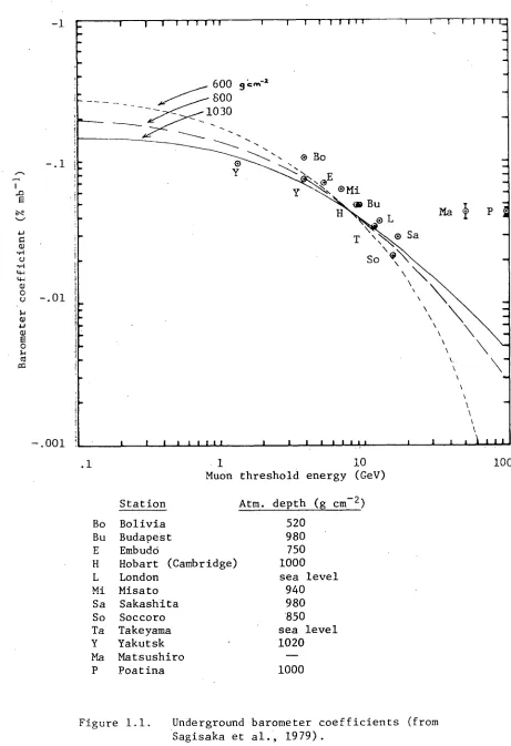
The solid and dotted curves give the expected pressure coefficient as a function of muon threshold energy and the atmospheric depth of observation. These curves were calculated by Sagisaka et al. using the theory of Dorman (1957) and Maeda (1960). The latitude dependence is very small, as the barometer coefficient is almost invariant with respect to geomagnetic cut-off rigidity. For example, a change in rigidity of 10 GV causes only about a 4% change in the coefficient for a vertical muon telescope at sea level.

From the results in Figure 1.1 it is seen that the empirical coefficients are systematically slightly larger than expected. This trend has continued with the results of underground observations at Poatina and Cambridge. The search for a reason for this phenomenon is the main subject of his thesis.

1.2 The Mechanism of Atmospheric Effects on the Muon Intensity

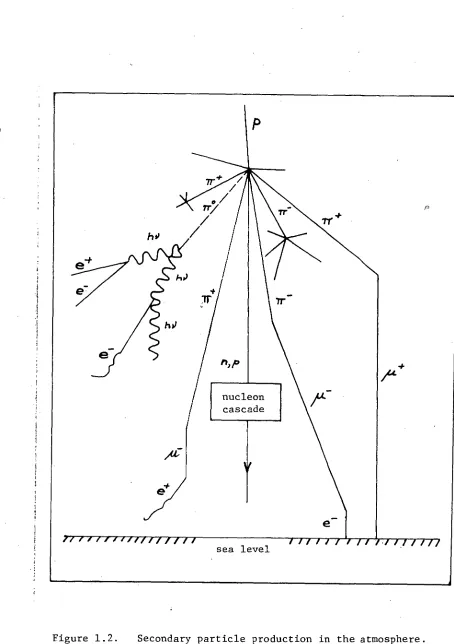
As a basis for later chapters, it is desirable to briefly review the production mechanism of the secondary component of cosmic radiation and the influence of the atmosphere on it. Figure 1.2 shows the typical nucleon-meson cascase which produces the muon.

On entering the atmosphere from interplanetary space, a primary particle (of which 80-90% are protons)

will most likely collide with an oxygen or nitrogen nucleus. Such interactions produce secondary particles such as pions, kaons or more nucleons. At low primary energies, the

5

Figure 1.2. Secondary particle production in the atmosphere. The horizontal scale is greatly exaggerated.

relative proportion of kaons to pions is very small, but this figure increases somewhat for high energy primaries

(?. 10 12 eV).

Most nucleons produced in the initial collision suffer further interactions, so producing more secondaries. However, the majority of charged pions and kaons decay

spontaneously to produce muons of the same charge, on a one-to-one basis. The charged pion is a short-lived particle having a rest mass of (273.27 ±0.12)m e , where m

e is the electron mass, and a mean proper lifetime of

(2.55 ±0.03) x10 -8 s. The charged kaon is heavier, at — 965 m_e, but shorter-lived at — 1.23 x10 -8 s. The most common decay processes for the two particles are

+ v

K --> p +v

The charged muon has a rest mass

of (206.86 ± 0.12)m e and a relatively-long mean proper lifetime of (2.20± 0.01) x10 -6 s. It decays according to the process

u - e +2v .

As the muon travels downwards through the atmosphere it loses energy, chiefly through ionization, at a rate of — 2 MeV cm 2 g -1 . The average flight energy of muons

detected at sea is about 3 GeV and the Lorentz-dilated lifetime of such a muon is about equal to its time of flight from its production to sea level. The maximum

2

165

7

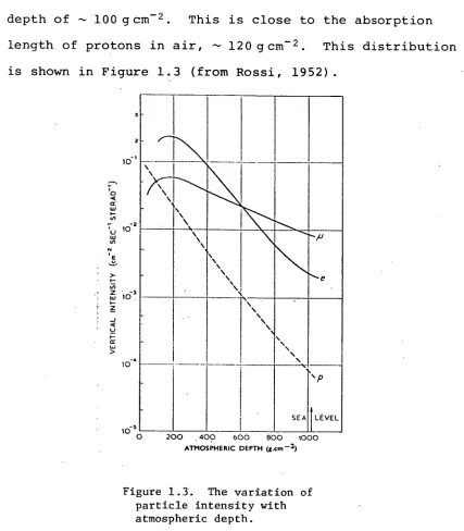
depth of — 100 gcm -2 . This is close to the absorption length of protons in air, —120 gcm -2 . This distribution is shown in Figure 1.3 (from Rossi, 1952).

\ \ - \ \ \ • \ \ \ \ \ • \ \ \ \ • \ ■ - \ \ \ \ \ \ \ \ \ \ \ \ SEA N. LEVEL

200 400 600 BOO 1000 ATMOSPHERIC DEPTH (g.cm —2)

Figure 1.3. The variation of particle intensity with atmospheric depth.

Early investigations by Mysskowsky and Tuwim in 1928 revealed a negative correlation between the intensity of the hard component of muons and surface air pressure. This is the mass absorption effect which predominates at low energies. The empirical pressure correction coefficient, b Ip , is

determined by the least squares process using the regression equation

8

where AI/Y represents the fractional change in muon intensity from some long-term mean, and AP is the corresponding change in pressure.

However, any increase in the production height H of the muons will increase their chance of decaying before reaching ground level. Therefore, a corresponding decrease in I is to be expected. At the same time, an increase in the temperature T around the pion production level causes a decrease in air density. This will increase the chance of pion decay per unit length, and result in an increase

in I.

Thus Duperier (1944,49) and others found that a

greater proportion of the variation in I could be explained using the four-fold regression equation

AI/Y = b

IP.HTAP + bIH.PTAH + IT.PHAT (1.2)

where the three coefficients are, respectively, the "partial" pressure, height and temperature coefficients.

The Duperior method of (1.2) has been widely used owing to its simplicity and freedom from possible errors which might result from using purely theoretical correction methods. Provided the intensity is reasonably correlated with each of the chosen variates, the method is sound for predictive purposes. This is due to the fact that for any given sample set (P,H,T,I). the least squares coefficients can be shown to account for more variation in I than any other method of estimation using the same variates

In the following chapters, the underlying theory and shortcomings of the least-squares method will be

examined in detail. It will be shown that the often-used dual aim of prediction and inference of an underlying physical mechanism may be unsound, particularly for muon observations at great depths underground.

CHAPTER 2

MATHEMATICAL NOTATION AND CONCEPTS OF LINEAR ALGEBRA

Most of the calculations in this thesis concern the analysis of, say, n observations made on p variables

simultaneously. The constant n is typically the number of days in a month and p is perhaps 3 or 4. The best way to describe such large arrays of numbers is through a

standardized system of matrix-vector notation which readily lends itself to any size problem. The following points are central to later chapters:

(i) Vectors are represented by underlined lower case letters, as in x, and denote columns unless otherwise stated.

• (ii) Matrices are represented by capital letters, as . in X and consist of, say, n rows by p columns, where the 3 th columnofXisdenotedx..A matrix may be partitioned

-3

column-wise, as in [Xi 1x21. The square brackets signify grouping where confusion might otherwise result.

(iii) A diagonal matrix D (say) is often denoted D = d1ag(dii,d22,...,d nn ) where the (i,j) th element is

• 6 d. - viz, off-diagonal elements.are zero. The identity matrixI is a special case where the d =1.

jj

(iv) The inverse of a matrix M (say) is M -1 and is defined by MM = MM- 1 = I . M is therefore necessarily square.

The transpose of any matrix X is XT, obtained from th

X by interchanging the (i,j) element with the (j,i)th, for all i and j.

Twocolumnsx.and x k of X are orthogonal if the -3

inner product Ic j .x k = jTx k = 0 . In the second form, the

vectors are regarded as (lxn) and (nxl) matrices respectively.

(v) In linear regression analysis the matrix product A =XTX is frequently encountered. It is by definition symmetric since a kj =a jk .

(vi) The eigensystem of a square matrix. If A is sonlepxpsquarematrix,theeigenvaluesA.(j=1,...,p) are the roots of the polynomial equation

det (A - AI) = 0

and the eigenvectors v of A are defined by the matrix -j

equation

Av. = A v.

The (column) eigenvectors are mutually orthogonal and may be assembled to form the matrix

V ' [vilv I Ivp]

(vii) The trace of a pxp matrix A is defined by

ID

tr(A) = a.. j=1 33

If A is symmetric with eigenvalues X j (j=1,...,p) where the X, are all non-negative, the following relations hold:

tr(A) = A. j=1 j

and

tr(A) = A tr(A -1 ) = X -1

j=1 j j=1 j

Furthermore, if A is diagonal, the elements are the eigenvalues of A. If X, are at least non-negative, A is said to be positive semidefinite, and is positive definite if X. >0 for all j.

7

(viii) If A =X T X we define the singular values of X by

E

1" ) 1

(ix) If x is a vector with n elements, the length or Euclidean norm of x is given by

IlII = x.x = x x = (x12+x22+... x2)2

_{- - - -}

(x) The supremum (sup) and infremum (inf) are, respectively, the lowest upper bound and greatest lower bound of a set.

12

13

CHAPTER 3

PREDICTED METEOROLOGICAL EFFECTS ON THE MUON INTENSITY UNDERGROUND

3.1 Approximate Methods

The Barometer Coefficient

The simplest calculation of this effect uses the intensity vs depth curve for muons. It is assumed that an increase in air pressure is equivalent to shifting the muon detector to an

appropriately greater underground depth. Therefore this method does not take into account the contribution of muon decay to the pressure coefficient, which is expected to play a small part at depths where the muon threshold energy is less than about 10 GeV.

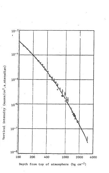
Barret et al. (1952) have collated the depth-intensity measurements of many workers; the results are shown in

Figure 3.1. The relation between the integral intensity and thickness of matter h takes the form

= I h -n

p0 (3.1)

where the exponent n varies from about 2.0, near the surface, to 2.2 for great underground depths. Differentiation of (3.1) with respect to h yields, for the mass absorption coefficient,

dl 1

13 1, (g cm -2 ) -1

dl dh

mb -1

=

1 dh dP n dh

-E1T- nhj

101 1O-3

1

100 200 400 1000 2000 4000

Depth from top of atmosphere (hg cm -2 )

Figure 3.1. The variation of muon intensity with depth underground (Barret et al., 1952).

For non-zero zenith angles 8 we have, provided n does not change,

15

-

P hsece • dP

n dh h dP = - 1.02 [ 11-11

since

dhsece

(3.2)

P[mbi = 0.981 h [g cm -2 ].

Therefore, the pressure coefficient is practically independent of zenith angle, as noted by Dutt and

Thambyahpillai (1965). However, it will be shown later

that at large depths, the coefficient tends to vary as cose, causing, for example, a semicubical telescope to see a

smaller effective pressure coefficient.

The analysis of data from Cambridge and Poatina, Tasmania, is the subject of Chapters 4 and 5. Using the

values (h,n) = (3.7 x10 3 ,2) for Cambridge and (3.47 x10 4 ,2.2) for Poatina, we obtain the following absorption coefficients for vertically incident particles:

Cambridge: 8abs - 0.055 % mb

Poatina:

abs - 0.0065 % mb -1

Trefall (1955) has shown that up to medium depths underground, a small additional component, due to muon decay, is present in the barometer coefficient. This arises from the fact that the survival probability of a muon will

16

its flight-path. An increase in air pressure will cause such a loss of energy. For Cambridge (threshold energy 10 GeV) the muon decay component amounts to - - 0.01 %mb -1 , resulting in a total barometer coefficient of - - 0.06 to - 0.07%mb -1 . At Poatina (threshold energy 100 GeV) the muon decay effect is negligible.

The typical day-to-day pressure range observed at the two centres is - 12 -15 mb. Therefore the barometer

effect is expected to be large at Cambridge but insignificant for deep detectors, such as at Poatina.

The Height Coefficient

An increase in the average height of muon production will increase the probability of muon decay before reaching the level of observation, leading to a drop in intensity.

The rest lifetime of a muon follows the negative exponential distribution

f(t) = (1/T )exp(-.t/T )

where T is the mean proper lifetime, - 2.2x 10 -6 seconds.

The geometric distance travelled by a muon in time t is then z = yT c, where y is the "average" Lorentz factor

over t and c is the speed of light. The survival probability of a muon created at height H=z is then

Pr(no decay) = exp(- z/z p )

and so the intensity of muons detected is

I = I

Differentiation of (3.3) yields for the height coefficient

17

1 dl

a H

I dz II

1

(3.4)

y T C 11

To evaluate (3.4),

T

+ AE + 2 [GeV] • 1

m c 2 [GeV] P.

(3.5)

where AE is the muon threshold energy. Insertion of the appropriate values yields the following height coefficients:

Cambridge:

▪

- 1.3 % km -1

Poatina: _13H - 0.15 % km -1

The typical diurnal fluctuation in H1 0 0 is — 0.3 km while the seasonal range is — 0.5 km. Thus the muon decay effect would appear to be small but significant for Cambridge but negligible for Poatina.

The Temperature Coefficient

As with the height coefficient, we assume that the temperature effect is characterized by temperature variations at the "mean" level of pion-muon production.

Barret et al. (1952), Pine et al. (1959)and others have shown that the probability that a pion with energy E Tr ,

(3.8) 6_T = I _{dT B +E}

TT 7T

dl E1

1 ii it

18

P

r(decay) B + E n Tr

(3.6)

where B is about 110 GeV and is proportional to temperature, 7

T. Thus B = k l T, say, where 1( 1 is some constant. The 7

muon intensity is proportional to the number of pion decays and may be written

I = I

po + E

Tr (3.7)

Differentiation of (3.7) gives for the temperature coefficient

The typical threshold energies at muon production for Cambridge and Poatina are 12 and 102 GeV respectively. Since T = 217 K (ICAO Standard Atmosphere) we have, for the temperature coefficients,

Cambridge:

T C-4 0.045 % K -1 Poatina:

T 0.22 % K -1

It is shown in the next section that the temperature coefficient tends asymptotically towards 1/T = 6.46 % K -1 as AE 00. Whereas at great underground depths the mass

19

3.2 The Integral Method for Calculating Atmospheric Effects on the Muon Intensity

3.2.1 Introduction

The expressions for atmospheric effects on muons have been developed by several authors, in particular Dorman (1957) and Maeda (1960). For this reason, the completederi-vations will not be repeated here. Instead a

simplified summary is presented, with calculations of the pressure and temperature effects for the Cambridge and Poatina detectors.

Fundamental assumptions are:

(i) The primary radiation consists of protons incident isotropically on the top of the atmosphere.

(ii) Secondary particles preserve the direction of travel of the parent proton. For muons with total energy E >1 GeV, the maximum angle between the pion and muon directions •is <2°. In turn, the angular deflection through scattering of muons at — 100 g cm -2 and energy 2 GeV is <10°. At higher energies the deflection drops rapidly, so that over all energies, — 98% of muons be within a cone 4° wide, centered on the original proton direction (Bolli, 1971).

(iii) A negligible fraction of the muons detected at sea level and underground is derived through the decay of kaons rather than pions. This assumption breaks down at higher energies (?, 30 GeV). Corrections will be

20

Consider a primary proton incident at zenith angle 0 on the top of the atmosphere. Let L denote the proton absorption length in air, 120 gcm -2 (Hook & Turver, 1974) and let y denote the exponent of the primary proton spectrum

(not to be confused with the Lorentz factor mentioned earlier). The differential proton spectrum varies as E -Y where y ,-, 2.65 over the range 10-10 4 GeV (Wolfendale,

1963) and is attenuated as exp(-hi/L p x) where 111 is the atmospheric depth of the proton collision and x=cose. The differential pion production spectrum is therefore

flr (E ,hi,x) = E -Yexp (-hi/Lx) (3.9)

where I is a constant.

The pion of absorption length L ir = 120 gcm -2 decays at depth h2 to a muon. Both pions and muons lose energy through ionization at a rate a= 2 MeV cm 2 g -1 as they traverse the air, but the total energy lost by a pion is negligible owing to its very short decay length.

A pion of energy E7 produces a muon of energy

E = a E where the mean value of a is 0.787 (see Appendix 2). 7

For a muon telescope with parallel-plane geometry, 0

such as a cubical telescope, the minimum pion energy at generation corresponding to an absorber threshold AE is

Emin = [AE + a(h 0 -h 2 )]/ax (3.10)

T m c

112 dh 1 p(h) 7 (3.12) h 1 J dh - m c

1 h2

21

ho

I (ho,AE,x) = dE dh2 f il2 dhl.F(E,hi,h2,h0,x)

E

min o 0

(3.11)

where F(E,111 1 h 21 110 1 x) =

It IT

.

- exp

m c f (E,hi,x) h2h1]

To proceed, assume that air obeys the perfect gas equation so that

PV = R'T where P = pressure, V = volume m = mass of air, M = mean

molecular weight of air = 28.97 x10 -3 , R' = 8.314 Jmol -1 K -1 and

T = absolute temperature (K)

Thus

M

P = I • ) •

But P[Nm -2 ] = 9.81 h [kg m -2 ] and so

or

p[kg m -3 ] - h[kg m -2 ] 29.25T

P[g cm -3 ] - h[g cm-2 ] RT where R = 2.925 x10 3 cm K -1 .

. exp [-

Ex j

exp [ p (h) aEx - a (h - h 2 )

(3.13)

To simplify (3.12), we may assume that the atmosphere is isothermal at temperature T. This is acceptable for underground telescopes. Define

22

m cR - n,p

P

(3.14) where

Then (3.12) becomes

TI -y-1

F(E,h1,h2,h0 1 x) = -1 0 E • exp -Lx

exp

[ f

h2 dh b

• -

h • Ex h l

exp [ -

I h0

dh

b

. P

h ctEx - a (h-h2) h2

' (3.15)

Expression (3.15) is substituted into (3.11) and the various atmospheric effects are derived by taking partial derivatives of (3.11) with respect to the different atmospheric parameters.

The Barometer Effect

Differentiation of (3.11) with respect to hp gives ] h i h 2 -h 1

23

+ dh o

From (3.10),

dE / E

.

(SE

(SIW=-6E.fdll2fdlli.F(E., 11 1,h2,ho,x) 11 0 h 2

min

0 0

m u c fh o h 2

dh l . 0

min

F(E,h 1 ,h 2 ,11 0 ,x)

T + . min dh 2 p(ho) 0 110

I dh1.F(E,h1,h2,h0,x) 0

a

aEx - a(h 0 -h 1 )

(3.16)

(3.17) -dh o

ax

which is substituted in (3.16). The right hand side of (3.16) is broken down as follows: the first term is the simple air mass absorption effect, while the second consists of two parts. The first of these expresses the contribution of muon decay to the barometer effect and the second results from variation in the number of pions being created. For detectors near sea level, or underground, the last part is negligible.

Choice of units

At this point, a certain choice of units will simplify further algebra considerably. As in Dorman (1957), we note that a = 2 MeV cm 2 over a wide energy range. At very high energies, a rises, but the ionization loss term

p/aEx fh2 I0E - exp(-h2/Lx)h2

dhl.F

0 l+ (Ex/b 7 )

(3.20) 24

The mass absorption term

(i) Integration over hl

Define

n _{= hi/h2}

01 = h2/XX

02 = b 7T /Ex where 1/X = 1/L -1/L 7

Then it may be shown that

(3.18)

fh2

dh 1 .F(E min ,h1,h2 1 h0,x) = h2

o

1

dn.FCE . n

0 mm

7

I 0 E -1 b b /aEx 1

. exp(-h /L 7 x).h 2 P fexp(nOn *2 dn (3.19)

where E.=Emin and muon ionization losses in the atmosphere have been ignored.

To a first approximation, L =L=L (say) = 0.12

(using our special units). Therefore 01=0 and (3.19) becomes

(ii) Integration over h2

fho h2 1

dh2 dh2.F = j dh2 1 112 dhl.F 0 0 0 0

1 0 E"

25

10E 1

1+b /aEx (1/Lx b /aEx

(Lx) P exp(-t)t P dt where t=h 2 /Lx

JO

1 +Ex/b u

1 0 E -1 f l/Lx

(Lx) Y . exp (-t) 07-1 dt where y = 1 + b a Ex 1 + Ex/bir ₀

(3.21)

Since 1/Lx »1, the integral in (3.21) approximates the "gamma function" which is defined by

r(y) E exp(-t)t Y-1 dt 0

r (y+1)/y where r (1)_-1.

-Thus

(l/Lx 1+b / Ex

I dtexp(-t)ty-1 = (Lx) P .r(1+10 /aEx) .

J0

(3.22)

Evaluation of b /aEx using (3.14) and the appropriate numbers yields —5 x10-11 and 5 x10-12 for Cambridge and Poatina

respectively, values which are negligible. Then

1 _{Io E}-Y

.Lx

dh2

)1(11) 2 dhi.F = 1 + Ex/b

0 Tr

(3.23)

Therefore from (3.16), (3.17) and (3.23), the final expression for the mass absorption term (which forms the numerator in the mass absorption coefficient) is

SI (1,AE,x) abs P

1 10 L E ITI l n

= - SE [ dh, f il2 dh l .F - • Shp min ) - )

0 0 a(1 +E . x/b ) _{min Tr}

26

(iv) Integration over E

This final integration is required to derive an expression for

I (h 0 =1,AE,x).611 0

which forms the denominator in the final formulae for the mass absorption and muon decay components of the barometer

coefficient.

From (3.11) and

I (1,AE,x) =

At high energies, y +3. Equation 2.118-3) comes

dx -1 =

(3.23)

dE E. _nun

IoLx

f'

E .

From the

1

dh 2 f h2 dhl.F 0 0

E" dE (1965, (3.25) (3.26) (3.27) (3.28)

rran 1 +

Ex/b

IT

Gradshteyn and Rhyzik standard integral

b2

ln [a + bx) f x3 (a+ bx) 2ax 3

We use the fact that at

E

Applying (3.26) to (3.25)

I (1,AE,x)

Finally, from (3.24),

a 2 x a3

higher energies,

= AE

. .

, _{x j}

3

(3.28) the mass

min ax yields

I 0 L bTrx3

-

3 AE

27

- 3x 1 61 (1,AE,x)

abs -

abs (1 'AE'x) = _{6h0 I (1,AE,x) b Tr + AE}

From (3.14), b ir a is negligible, leaving

abs (1 ' AE'x) =

-3x

AE (1000 g cm -2 ) -1

-0.6x AE[GeV]

-0.6x AE [GeV]

% (g cm-2 ) -1

% mb -1 (3.29)

The muon decay term

We consider the first part of the second term in (3.16). Since a(h o -h 2 ) « aEx we may again ignore ionization losses and the expression becomes

- 61-10 m u c f_w 1 h2

dE _{dh 2 dh .F} f

SI (h0 =1, AE , x)

decay

T p(h o )ax E 0 0 min

E-(y+1) - h o mp c

dE (3.30) a t p (h0) - 1 +Ex/b _E.

TT min

Again, y=3. The expression may then be simplified using another standard integral (Gradshteyn and Rhyzik, Equation 2.117-4):

[l

dx = -1 b 2 b 3 a+bx _{in (3.31)}

28

Using (3.30) and (3.31) where the lower limit of the integral is again E min = AE/ax, the decay term simplifies to give

6I(1,AE,x)

p decay

-Th o m cI o L x 2 b a 3 • Tr

T p(ho) 4 AE

(3.32)

Then from (3.12), (3.14), (3.28) and (3.32), the muon decay coefficient is

B _decay(1,AE,x) =

1 (1,AE,x)

p decay

dh o ' I (1,AE,x)

-3 m c

4E T p(ho)

m cRT

(1000 g cm -2 ) -1

% (g cm -2 ) -1

% mb -1 4 AET

0.102

AE[geV]

0.1 =

AE [GeV]

(3.33)

The complete barometer coefficient for an underground detector

with threshold energy AE ?_10 GeV is then

(31,(1,AE,x) = (0.6x +0.1) mb -i

AE (3.34)

P

a

Jo

RS(x)dx 0

Estimated Barometer Coefficients from Cambridge and Poatina

To obtain the barometer coefficient seen by an actual telescope having a finite viewing cone, it is necessary to integrate the directional (x-dependent) coefficient

6(1,AE,x) over the radiation sensitivity function of the telescope. This function is denoted

RS(x) = GS(x)x n

where GS(x) is the geometrical sensitivity function of the instrument and x n represents the angular distribution of muon intensity. The best-fit value of n is —2.2 for 6 up to —70 0 (Parsons, 1959) - viz. x down to 0.342.

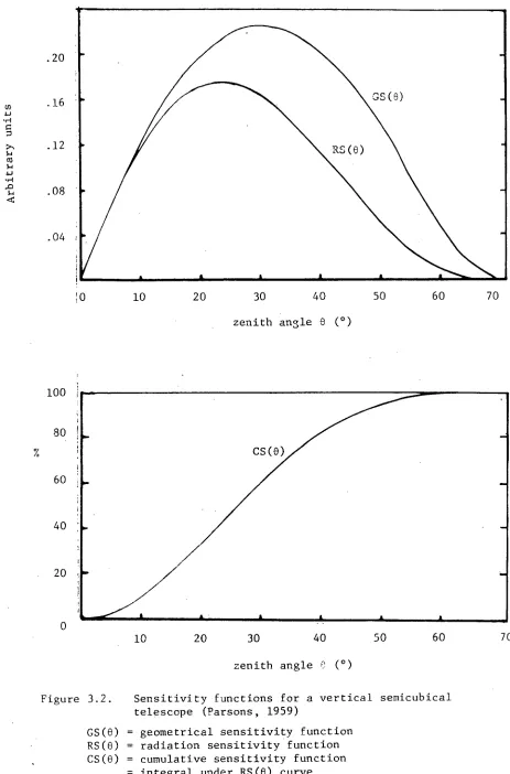
Calculations of RS(0) for various telescope geometries and tilt angles have been carried out by Parsons (1959), Lindgren (1965) and others. Figure 3.2 shows the RS(6) and

Gs(e) dependence over a vertical semicubical telescope

(Parsons). It is seen that the RS(6) curve reaches a maximum at about 23°.

Reverting to the RS(x) formalism, the aperture-integrated pressure coefficient seen by an underground telescope is then

29

(3.35)

, For Cambridge and Poatina, substitution of the

30

and -0.007 % mb -1 respectively, for vertically incident muons. These values agree quite well with those predicted

by the simpler method in Section 3.1. However, as already pointed out, the dependence on x in (3.34) is not valid for small values of AE (such as at Cambridge). The latter formula is only approximate for small depths underground where muon energy losses due to ionization cannot be regarded as

. negligible, and y is somewhat less than 3.

Thus the integrated barometer coefficient for Cambridge, for virtually any telescope geometry and angle of tilt, will be

(1,AE = 10 GeV) - 0.07 % mb -1

Camb. (3.36a)

To obtain the integrated pressure coefficient for Poatina, a cubic spline was fitted to RS(x) and (3.35) evaluated numerically with (3.34) substituted in. The result obtained was

(1,AE = 100 GeV)

Poa. - 0.003 % mb -1 (3.36h)

[N.B. More significant figures are meaningless in view of the approximation y=3 used to obtain 3.34.]

3.2.3 The Temperature Effect

Case 1: Small Depths Underground

As for the barometer coefficient, for underground

31

accuracy, the muon energy loss term - (h-h 2 ) in equation 3.15 will not be dropped in these calculations. As will be seen later, the temperature coefficient varies with atmospheric depth and omission of the energy loss term distorts the shape of the curve for low to medium cut-off energies.

Differentiation of (3.11) with respect to T gives

fh 2

(SI (1,AE,x) = dE I dh2 dh 1 .F(E,h 11 h 2 ,1,x) E

in 0 0

m

(sT b ff fh2 dh ST 1 dh (ST

• — - — — — - bp

f

T Ex

h h 2 i h T T.h aEx-(h-h 2 )

(3.37)

where, again, a = hp =1. The first two terms in the brackets in (3.37) represent the positive temperature effect which is caused by competition between pion decay and interaction. The third term represents the negative temperature effect which is due to the effect of atmospheric expansion on the probability of muon decay.

(i) Integration over h l

fh 2

ST dhl.F. -7317

(

In dT b ETr

• —

-(y+1)

exp(-h 2 /L iT x) -exp [- 1

dh

h

h2

exp(mp l)n tP2 dn

I n b ST -

• - •

1 dh

h aEx - + h2 h2

exp(-h 2 /Lx) exp

I

+ b Tr / E x j

32

0

(3.38)

where again we let L=L =L so that tp l vanishes. The argument in the second exponential in (3.38) may be simplified using the following method:

Lett=E.

n/E= (1 -h 2 +AE)/aEx mi

aEx = (1 - h 2

1 _dh

Thus ii

h 2 aEx - h + h2

• b t

1

dh th2 -kh

2

where k = 11 0 -h 2 (1 -t) +AE .

Using the standard integral

Jdh _

in b + 2ch - /7-7A 1

b + 2ch +

fh2

dhl.r. , (ST (ST ₌

I0bE

T T . exp( h2/Lx) .

0

exp(vt) b 7

(ST [13 ) 2 I0 E -Y h2 7

.exp

T Ex h2 Lx

dh

h aEx

i

33

b t _{1 - h2}

in [h 2 (1 t .

h0 - h2(1-t) +E 1 - h2 +AE )

1 - h 2 1.1

= vt where v - in [11 2 11 -t.

h0 -h2(1-t) +AE 1 - h 2 +AE )

(3.39)

Thus (3.38) simplifies to

(ST -

T .I 0 E Y exp(-h 2 /Lx)exp(vt)

(3.40)

Integrating the second term in brackets in (3.37), we have

f h2 b (ST h2

dh]

d

l .F [- —I --

--

h

0

111

(ST b hi

dhl.F.ln (— h

) - 2 T EX J 0

[ 1111 11b 7 /Ex [hi) fh2 dhl

J in --

2 h2

Again, letting n=hi/h 2 and 11)2 =b 7 /Ex, the last factor in the expression above becomes

( 1

h2

I

)1:1

in n

- h 2

(1 + 4)2) 2

h2

(1 + b7r/EX) 2

so that the complete expression is

2

5T b

- I4—

E71) E-1 exp(-h2/Lx)exp(vt)

T x

b ) 2 [1 +

Ex

(ST —

--- 1 0 E 1 exp(-h2/Lx)exp(vt)

(3.41) Ex) 2

[1 + 13-

7

The total positive temperature effect is then found by adding (3.40) and (3.41):

34

6T _

0

-Y

E 'exp(-h 2 /Lx)exp(vt)

-if

-

Y

AI

(3.42) [ 1 Ex l b7)

Ex

35

h2 1

óT dh 1 I dhl .F [- b

1.1 T h aEx - h +h2] 0 h2

1 f

0

h2 I ST dh

= - .F

h • aEx - h + h 2

2

ST

y

exp(-h2/Lx)exp(vt) 1

T b

i _P

h • aEx -h + h 2 Ex

1 + _h2

b

It

(3.43)

by virtue of (3.40).

(ii) Integration over E

(a) Positive temperature effect

We require a simplified expression for

-

dE . ST I E exp (-h 2 /Lx) exp ( vt)

Emin

E Apply again the change of variable t -

E '

E . x 1 - h 2 + AE mmn

ab

Tr TT

[ Ex b

1 + [1 + —II b Ex j

Tr

(3.44)

and define

(3.45)

36

ST

[LX]

r1

[

t y-1 s

t+sj exp(vt)dt 1 1 2

I0 exp

.

E .) 0 min

45 T

-

10 a y-2 x y .exp(-h2/Lx) -1

G

ty-1 exp(vt)dt

T

ST 0

b 71. ( 1 - h 2 + AE) " 2

y-2 -1

y

a x exp(-h 2 /Lx)

. (s,v)

(t+s) 2

b (1 - h2 + AE) " 2

TT (3.46) where Thus 1 tY-1 s, v ) =

JO

exp(vt) dt (3.47)

SI (1,AE,x) pos.

1 _{WT * (h2,1,AE x)}

. ST dh 2 (3.48)

dT

where the numerator W

T of the integrand is the expression (3.46). Since variations in intensity are usually expressed as relative changes from the mean, we require an expression for the total directional muon intensity.

total

To obtain an expression for I (1,AE,x), we have

total

(1,AE,x) = dEf

h2

h dh 2 I ( dhl.F E . 0 )0

min

-h 2

I 0 E Y exp6d exp(vt)

= I dh 2 f m dE .

0 E min , EX + b,T -h2 exp (s,v)

= I 0 (ax) Y-1 dh 2

where

H (s,v) =

using the same methods employed

Itotal (1,AE,x) u

where

D (1,x) =

Finally, dividing (3.48)

[51 = 1 t Y-1 exp(vt)dt Thus (3.49) (3.50) (3.51) (3.52) (3.53)

0 t + s

in deriving (3.46).

= I0 (ax) D (1 y , x)

1 _{exp(-h2/Lx).H (s,v)}

dh2

J

o

by (3.50) yields

1

WpT (h,l,AE,x)6T(h)dh os 0

exp(,h/Lx).Gy (s,v)

( 1,AE,X)]

I (1,AE,x) Ii pos

where

os

WP (h,l,AE,x) =

aTb (1 - h + AE) " 2 .H (s v) _It

WT (n 1,AE,x) is known as the "positive temperature

coefficient weighting function" and specifies the temperature influence, due to pion decay, of a differential layer of the atmosphere [h,h+dh] . (The "2" subscript On h2 has been dropped as it is now just a dummy variable.)

(b) Negative temperature effect

A simplified expression is required for

and s -

7

Ex 1 + To—

Emin . x f' dE

E . min

ST

7.17 I0E Y exp(-h2/Lx)exp(vt)

( 1 dh

) h • aEx -h+ h 2

h2

integration of (3.54) 38

E. min Again using t -

over terms dependent on E will be

1 dt.E

min I

f —

)Y 1 1

min t +s 1 - h 2 +AE - t(h

-h ) exp(vt) 0

1 f 1

1 h ) at

ax t Y 1 1

t+s h - h2 • 1 - h 2 + AE 0

- 2 + AE

h - h2

exp(vt, ti

(ax) y-1 1

0 K dt• = ktY exp(vt) k -

1 - h 2 + AE

(3.55)

(3.56) (1 - h2 + AE) Y

(ax) Y-1 . (s,k,v)

(t+s) (k-t) where

( 1 kt Y exp(vt) dt

h - h 2

(1 - h2 + AE) Y

where

K (s,k,v)

Jo (t+s)(k-t)

Thus

1

ST (ax) Y-1

= - To 71, b o dh2

(SI (1,AE,x) neg

0 (1-h2 + AE)

1 K (s,k,V)exp(-h2/Lx) f dh

h2

1

w neg

(h)dh (3.58)

[61 (1,AE,x)] I (1,AE,x)

p .

39

1

1 1 (h

(

dh 2 I dh + dh dh 2 la

0 • 0

2

Applying this, we get

(1,AE,x)

neg = -

f

0

1 611 Io q

P(ax) "1 dh

fh K y (s,k,v) exp(-h 2 /Lx) dh2

jo (1 - h 2 +E) 1 (3.57)

Division of (3.57) by (3.50) gives

where

neg ( h, 1, AE,x) _- W

T

_ q

₁

y I (s k v)exp(-h 2 /Lx)

dh2 D (1,x)h 0 (1 -h2 +AE) 1

(3.59)

The complete temperature weighting function is then

W (h,l,AE,x) = W TP°s (h,l,AE,x) wneg n ±,AE,x) (3.60)

for muon telescopes at or below sea level. (Again, h 2 becomes h, in the interests of simplicity.)

Case 2: Large Depths Underground

threshold energy and we can use the simplified expression for the total directional muon intensity:

I (1,AE,x)

I o Lb x 3 a 1 3 1T

3 AE )

(3.28)

(a) Positive temperature effect

In (3.38), the second exponential becomes

J

1 b p ]

exp [- = exp ln h 2 ]

h aEx [aEx

112

b /aEx = h2 P

= 1 since, for example at Poatina, b /aEx. <5 x10 -12 for vertically incident muons.

1.1

dT

I0E Y exp(-h2/Lx) Thus (3.42) becomes

E is then

. Integration over ( 1 4. Ex) 1 1 bTrl

Ti Ex)

(ST

—T— I 0 exp(-h 2 /Lx)

dE

y 4. Ex) [ 1. b 7) E

min E' _Tr Ex

b x 2

Tr f a SI

I exp(-h2/Lx).

k

T E )

3

where y=3

(3.61) Division of (3.61) by (3.28) yields

40

pos W

T -

exp(-h/Lx)

41

(b) Negative temperature effect

Integration of (3.37) over h l will be:

h2 f

'ST dh 1 ] dhi .F[-b

T h aEx 0 h2

b /aEx dT -y

P 1

_ IcIE b exp( - h2/Lx)h2 11 f dh h Ex

1 + h2

b 1r

Using the change in the order of integration, the integral over h2 is then

dT

I 0 E-1 b 1

dh 1 h b /aEx

dh2.exp(-h2/Lx)h2 P h aEx )

Ex ₀ 1 +

it

Using the change of variable t=h2/Lx, Dorman (1957) shows that the final integral is approximately

Lx[1-exp(-h/Lx) provided bp/aEx «1 .

Integration over E then proceeds:

dE dT _{1 0 Lx [1}

- exp (-h/Lx)

T

hax E1+1 ( 1 + Ex)

min Tr-

x 2 b a ) 3

ST

Lx [1 - exp (-h/Lx) — .

T

4 AE AE

(3.63)

42

Division of (3.63) by (3.28) gives

q,

'[1 - exp(-h/Lx)] neg

W_T (h,l,AE4-c°,x) _hAE (3.64)

(c) Asymptotic Behaviour with Energy

From equation 3.62 , the positive temperature weighting function reaches a maximum at h = 0 and is independent of AE

when AE is very large. Consider a uniform change in temperature dT = 1 K over the whole atmosphere. The

"integrated" positive temperature coefficient will be

1

,pos

(h,l,AE,x)dh = - 1

T e [ xp(-8.3) -1]

) "

0

= K- (3.65)

where L=0.12 atm = 120 gcm -2 .

Inserting T=217 K (ICAO Standard Atmosphere) yields an upper limit of 0.46 % K -I .

Meanwhile from (3.64), at high muon threshold energies the negative temperature effect becomes negligible. For

neg

example, for h = 100 gcm - 2 and AE GeV, vi T (n) <- 7 x10 -15 % (g cm -2 ) -1 K 1 .

WI Predicted Temperature Coefficients at Poatina and Cambridge

43

a reliable long term coefficient can be obtained via regression analysis. However, representing the temperature effect as a single coefficient assumes that all pion production occurs at some discrete level (such as 100 nth) , or over an interval of pressure whose temperature might be represented by a weighted mean, computed from the measured temperature profile. Clearly, this assumption is rather crude since the temperature effect is a continuously varying function of pressure. Therefore the "temperature coefficient" is a somewhat ill-defined concept where the only practicable criterion for selecting the "best" one is to choose the one that gives the highest R 2 value in the regression.

For underground muon telescopes, the effective

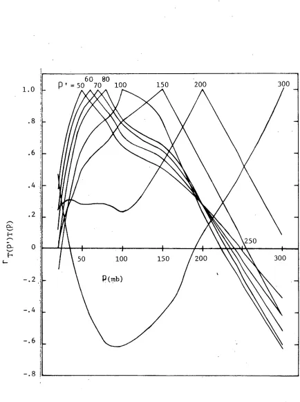
temperature coefficient will depend on the consistency of temperature variations in the stratosphere. To investigate temperature intercorrelations in the upper atmosphere,. Hobart weather data were analysed for the period 1972-77. Using daily mean temperatures, the correlation matrix for 11 levels over the interval [20,300]mb has been computed and the results are shown in graphical form in Figure 3.4. The most

important features are that temperatures tend to vary in the opposite sense above and below the tropopause, while consistent behaviour is found in the stratosphere. Thus, for high cut,-off energies, it would seem that there is nothing to be gained by using a weighted temperature that includes temperatures from the lower atmosphere. Such a coefficient would be smaller than one computed using

44

In view of these facts, theoretical prediction of the coefficient is difficult. The temperature weighting function for Cambridge has been computed using the low-energy formulae

(3.53) and (3.59), while for Poatina the curve has been calculated using the high-energy formula (3.62) only. The aperture-integrated curves have been obtained using

I

W

WT " (h 1 AE) =

1

I

where the radiation sensitivity curves are shown, as functions of 0, in Figures 3.2-3.3. The variation of

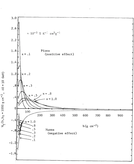
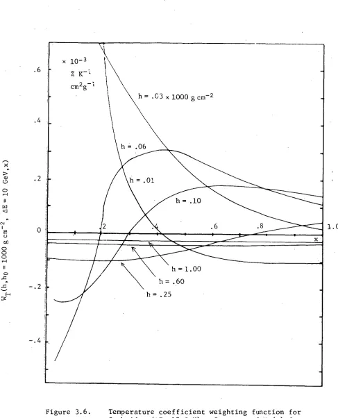
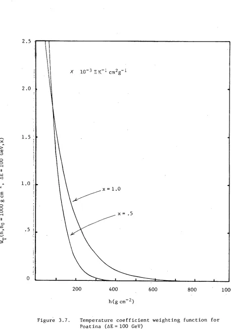
WT (h,l,AE,x) is shown in Figures 3.5-3.7 while the final aperture-integrated curves for the two sites are given in Figures 3.8 -3.10. Included also, for comparison, is the

curve for a vertical semicubical telescope which has operated at Cambridge.

To obtain the Poatina and Cambridge 70 0 zenith

temperature coefficients, the curves in Figures 3.10 and 3.8

.respectively have been integrated over the interval [25,200]g

cm-2 . These values were chosen as acceptable outer limits, based on the behaviour of the upper air correlations in Figure 3.4. The resulting coefficients are shown in Table . 3.1.

(e) The Influence of Kaon Decay on the Temperature Coefficient

TABLE 3.1

Temperature coefficients integrated over h= [25,2001gcm -2 . Units are % K- I

•

Positive effect Negative effect Sum

Cambridge 0.0619 - 0.0397 0.0222

Poatina 0.252 Negligible 0.252

The Poatina value agrees closely with that predicted by the simple method in Section 3.1. However, the negative effect is appreciable at the relatively shallow depth of Cambridge, resulting in an overall coefficient considerably smaller than that previously estimated.

TABLE 3.2

Charged kaon decay modes

Mode Fraction of decays (%)

45

K p + v 63

K

•

n + Tr° K -4- 7 - + n - + 7

T

+ + +

K -

•

7 - + 7° + 7°

Other 8

21

46

proportion of charged kaons produced in primary interactions increases with energy. Burcham (1973) has listed the main decay modes of the kaon; the more important are given in Table 3.2.

At 100 GeV the mean decay length of a _{K± is -0.75 km,} compared with -5.4 km for a Tr+ If the overall kaon

parentage of observed muons were large, a reduction in the size of the positive temperature effect would be expected. The K:n ratio at these energies has been estimated by Barish et al. (1973). A target was bombarded with protons and the resulting secondary hadron beam tuned for positive particles of energy -160 GeV. Of 112 neutrino events, 94 were identified as being of pion parentage and only 18 of kaon parentage . Although the errors are not aiven, from this evidence

it seems reasonable to expect the "kaon effect" to have only a small influence on the positive temperature coefficient.

3.3 A Monte-Carlo Simulation of the Temperature Effect at Poatina.

3.3.1 Introduction

In an alternative estimation of the temperature coefficient at Poatina, a Monte Carlo simulation of the proton-pion-muon

chain was carried out. The theory of the method is outlined in Appendix 1. Following standard practice, each run of the computer program begins with the injection of a given number of primary protons on the top of the atmosphere. The history of each subsequent pion and muon is traced down through the

TABLE 3.3

Assumptions used in constructing the Monte Carlo model

47

Angular distribution of primaries

Form of differential' primary spectrum

Proton interaction length, gcm-2

Proton inelasticity

- Charge ratio of pions 1.10 :ff

+ :TT

Isotropic

-2.7

E

P dEP

80

0.5

1:1:1

Charged pion multiplicity = 2 E 0'25

Pion interaction interaction length, g cm-2 100

atmosphere and rock overburden, until the muon is finally absorbed, decays or is detected.

To simulate the temperature effect, a step-wise

temperature perturbation of 20°C was applied to the interval [0,1501g cm -2 below the top of the atmosphere.

3.3.2 Results

17ifteen simulations were performed, each beainning with the

injection of 50,000 primary protons. Each run used a different number to initialize the random number generator. Five runs were performed for zero temperature perturbation, five for +20°C and five for - 20°C. The resulting weighted mean

b

temperature coefficient was

b

IT =(0.22 ± 0.05)% K -I

48

Ar

b

itr

a

ry

u

n

its

.20

.16

.12

.08

.04

10

100

!

60

40

20

70 60

50 40

30 20

10

zenith angle 0 (°)

0

10 20 30 40 50 60 70

zenith angle •(°)

Figure 3.2. Sensitivity functions for a vertical semicubical telescope (Parsons, 1959)

GS(8) = geometrical sensitivity function RS(8) = radiation sensitivity function CS(8) = cumulative sensitivity function

49

(GS) (RS)

.3

GSM .6

RS(8)

.4

1 .2

Ar

bitra

ry

u

n

its

50 60 70 30 90

Zenith angle 0 (°)

50 60 70 80 90

Zenith angle 8 (°)

60 80

=

Figure 3.4. Temperature intercorrelations in the upper atmosphere. Source: daily mean temperatures, Hobart Airport radio-sonde data, 1972-77.

200 300 400 500 600 700 800 900

.8 .5 3.0

2.61

x 10 -3 % K -I cm 2 g -1 2.2'

Pions

x=.1 (positive effect)

x= .2 1.8;

-1.6.

h(g cm -2 ) Muons

(negative effect)

100

; 1 •

x =1.0

. 3 . 2 .1

Figure 3.5. Positive and negative temperature coefficient weighting Functions for Cambridge (6,E= 10 GeV)

52

Figure 3.6. Temperature coefficient weighting function for Cambridge (AE = 10 GeV). Contours of WT(x) for

X 10-3 % K-1 cm2g- 1

600

200 400 800 1000

2.0 2.5

x = 1.0

x= .5 1.5

1.0

h(g cm-2)

53

.8

.6

-1.0

Pions (positive effect)

Muons (negative effect)

54

x 10-3 % K-I cm 2

Sum

200

400 600 300

h(g cm -2 )

Figure 3.8. Aperture-integrated temperature coefficient weighting functions for the Cambridge 70°

x 10 -3 K-1 cm 2 g -1

Pions (positive effect)

Sum

200 400 60

h (g cm -2 )

Muons (negative effect)

Figure 3.9. Aperture-integrated temperature coefficient weighting function for the Cambridge vertical semicubical

telescopes.

6

5

4 )(10

cyo 3

K-1

cm2g-1 2

0 100 200 h (g arr2 )

Figure 3.10. _{Aperture-integrated temperature coefficient} weighting function for the Poatina vertical semicubical telescopes.

56

CHAPTER 4

CALCULATIONS OF ATMOSPHERIC COEFFICIENTS FOR HIGH ENERGY MUONS

4.1 •The Equipment

The calculations described in this chapter concern muon observations made on underground detectors located at Poatina and Cambridge, Tasmania. Poatina is located approximately 130 km north of Hobart at latitude 41.8°S, longitude 146.9°E. The equipment is situated in an underground hydro-electric power station at a depth of — 357 hg cm-1 below the top of the atmosphere (Fujii and Jacklyn ). This corresponds to a median primary energy of — 1200 GeV. The muon threshold energy as calculatedin Appendix 1 is — 101 GeV. The

detectors consist of three vertical semicubical Geiger counter telescopes totalling 3 m2 sensitive area. Continuous observa-tions began in late 1971.

The Cambridge equipment is located in an abandoned railway tunnel 10 km north-east of Hobart at latitude 42.8° S, longitude 147.5° E. The observation depth is — 47 hg cm-2 which corresponds to a threshold of —10 GeV. A variety of detectors operate, or have been operated in the station. The calculations in Section4.4 of this chapter relate to a

narrow aperture 70 0 zenith angle telescope which was operated for the duration of 1964. The inclined depth of this telescope was — 140 hg cm-2 below the top of the atmosphere, which is equivalent to a threshold enercv of — 40 GeV.

1••• •••••••

140 ° E 145 ° E

•

Wagga • Canberra Mildura

Adelai e

'New South Waled

'Victoria'

0!Mt Gambier Laverto

40°S • Essendon

Bacchus • Marsh

0 Laverto

Aspend le

100

140 ° E

Melbourne

200 300 'Tasmania'

et.lobart an Cambr'dge

400 km 150oE

Sydney

South ! Australia

35 ° S 58

59

The location of the stations is shown in the map, Figure 4.1.

4.2 Least Squares Estimation

4.2.1 Two or More Regressor Variables

As a basis for the theory to follow, it is appropriate to review briefly the ordinary least squares (OLS) linear

regression model used for calculating atmospheric coefficients. The following theory is summarized mainly from Draper and

Smith (1966) and Seber (1977).

Multiple linear regression is a technique used for

finding the linear combination of atmospheric variables which best approximates the observed variations in muon intensity. The model then takes the form

'i i. = x₁ 1 1 x + + x (3. + i •

1 1 i2 2 _{iP P}

(i = 1, . ,n)

This is far more conveniently expressed in matrix notation as

(4.2)

where Y is an (nxl) column of muon intensity readings, X is an (nxp) matrix of n observations on each of p regressor variables (atmospheric parameters); f3. is a (pxl) column of regression coefficients, and c is an (nxl) column of

uncorrelated errors on Y, distributed with mean zero and variance 02 Note that (4.1) does not include an

Poisson.

intercept term SA as this is not normally of interest in the cosmic ray context; we are interested only in changes in Y from its mean as a function of changes in X from its

60

mean. In all further discussion it is assumed that the Y and X variables have been "centered" to have zero mean.

The OLS. estimator for 8 is

(xTx) - ' xTy (4.3)

where

E(Y) = Y = E() = (4.4)

and XT is the transpose of X, i.e. the estimate of 8 is

unbiased.

R

The vector of errors c is estimated by

e = Y -

= Y - (4.5)

called the residual vector, and the minimum residual sum, of squares (RSS) is given by

RSS = eTe = (Y - Xil)_{_ _} T(Y -

= YTY - 8 X Y . _{_} -T T

The total sum of squares of the response variable is

TSS = YTY .

(4.6)

(4.7)

By subtraction, the "regression" sum of squares must be

-

61

The quantity

R 2 = Reg SS/TSS = 1 - RSS/TSS (4.9)

is known as the coefficient of determination and expresses the fraction of the total variation in Y which is accounted for by the model. R is the multiple correlation coefficient between Y and X.

The variance-covariance, or dispersion matrix of fj, is given by

D() ₌ 0 2(xTx) -1

(4.10)

and therefore

var(.) = 0 2 (X T X) -1

' (4.11)

Estimation of 0 2 .

It may readily be shown that

2

= RSV (n - p - 1) (4.12)

is an unbiased estimate of 0 2 ; viz. E(s 2 ) = a 2 . If s 2 = 0 2 the model is inferred as correct and the chosen regressors are regarded as a complete set of explanatory variables. If

2 2

S >a the model is said to suffer from lack of fit. It is important to note that even if s 2 = 0 2 , R 2 may still be poor

(low). This merely indicates a large amount of random fluctuation in Y.

4.2.2 One Regressor Variable

The simplest case is the straight line. Again we are

(flx1) (1x1) (nx1)

62

Y.=13

1x. + E. , (i = 1, . ,n) (4.13)

or in matrix terms

(4.14)

As before, E i —(0,0 2 ). The OLS estimate of 131 is

T -1 T 6 1 = (x x) _{_ _} x Y

(4.15) I x.Y. / x. 2

11 1

i=1 1=1 .

and its variance is

var(l) = 2 -1 Tx)

(4.16) 0 2 / Z• x

i i=1

2

The coefficient of determination is equal to the squared correlation coefficient between Y and x:

R2 = r2= _{= X} (_{Y/ X} T TA _{x Y Y)}

(4.17)

= _{x jY i ) 2 / (E x. y. 2 ) E}

•

Comparison of (4.15) and (4.17) yields

(4.18)

where s and s

63

Point of Notation

For the remainder of this thesis, when discussing

regression coefficients on a conceptual level, the conventional 6. notation is used, as in the previous section. However, in discussing specific estimates obtained from actual calculations,

the following system may be used as it is more informative. Estimates are denoted by a "b" followed by a number of subscripts, as in

HT "b_

1 P. ". This example denotes the partial intensity — pressure slope where the remaining explanatory variables are height and temperature. Thus, for example, b

IP.T and bIP.HT are readily distinguished as coming from

different models, even though they are dimensionally the same. Furthermore, estimates in the "b notation" will be in

customary cosmic ray units of % mb -1 , % K -1 , etc. whilstestimates in "f3 potation" will usually correspond strictly to the

original units in the X and Y data. The relationship between the two is then

(4.19)

where

Y

4.3 Atmospheric Coefficients at Poatina

4.3.1 The Total Barometer Coefficient

64

against daily mean pressures over a five-month period. In all cases, each daily mean was obtained from 24 hourly readings; missing values were interpolated. The value obtained was b

IP = - 0.057 % mb -1 . This is much larger than the value obtained from the depth-intensity curve for muons on the assumption that an increase in pressure is equivalent to taking the muon telescope to an appropriately greater underground depth. The latter method yields

-0.007% mb -1 (see Section 3.1).

Alternatively, an estimate may be obtained using the integral theory in Chapter 3. From Equation 3.29 we have, for great underground depths,

- 0 . 6 cos()

% mb -1 AE(GeV) °

which for Poatina gives -0.006 % mb -1 for vertically incident particles. Integration of the radiation sensitivity curve of a semicubical telescope reduces the value to —0.003 % mb -1 ,

which is very small indeed. A longer-term analysis by Humble et al (1979) for the years 1972-76 yields the value (-0.047 ± 0.002) % mb -1 . This figure represents a weighted mean of 60 monthly coefficients'. Division of the data into separate monthly intervals was considered necessary to help eliminate the

confusing effects of long-term drifts in telescope efficiency. This trend is shown in Figure 4.2.

860

820

780

740

700

660

620

1972 1973 1974 1975 1976 1977

To investigate this possibility, time variations were examined in the coefficients for the period 1972-76. Figure 4.3 and Table 4.1 show the results of an harmonic analysis, the theory of which is summarized in Appendix 4.

Because of the relatively low count-rate, diurnal and semi-diurnal variations can barely be distinguished.

However, there is a very large seasonal variation, confirming that pressure cannot be the only atmospheric parameter

responsible for the intensity variations.

4.3.2 Partial Atmospheric Coefficients

Under the assumption that a Duperier-type multiple regression model is appropriate, a four-fold model using the following regressor variables was tried:

1. Surface pressure, P

2. Geopotential height of the 100 mb level, H100 3. Temperature of the 100 mb level, T1 00 .

The aerological data were obtained from the Bureau of Meteorology computer records, which are compiled from

radio-sonde flights made at Hobart Airport at — 1100 UT and — 2300 UT daily. The average maximum height of ascent is about 40 mb for these flights, which typically last for two hours. The launch site is about 135 km from Poatina. Thus there is a possibility of regressor error resulting from this separation. This question is examined in Section 5.3.3.

Weighted running means from three successive readings

of H100 and T 10 0 were used to calculate the daily means of these variables, whilst 24-hour daily means were used for