Statistical methodology for tab charts : data reduction techniques in laser ablation analyses

(1)

Department Of Mathematics

Statistical Methodology for Tab-Chart

s

: Data Reduction Techniques in Laser

Ablation Analyses

by

YUNG

,

Chi Ho

,

BA(Hons), MSc, MA

Submitted in fulfilment of the requirements for the Degree of

Master of Science

(2)

Acknowledgements.

I am deeply and greatly indebted to my supervisors Dr Des FitzGerald and Dr Peter

McGoldrick for their valuable advice and encouragement. I am also thankful to those

(3)

Al.Jt~orit~

Of

Ac:c:~

.

ss

This thesis may

be

made available for loan and limited copying in accordance with

the Cop

y

right Act 1968

.

YUNG, Chi-ho

(4)

Declaration

Except as stated within this thesis, it contains no material which has been accepted for

the award of any degree in any university. To the best of my knowledge

,

this thesis

contains no material previously published or written by other people, except where

due reference is made in the text of this thesis.

YUNG

,

Chi-ho

(5)

, Thesis Abstract

The researchers in the CODES and the School of Earth Sciences operate a laboratory to study the composition of rock samples, which are collected from the field site. The rock samples are put into a machine. This machine will create series plots of all elements (called tab-chart), which indicate the distribution of elements in the samples. In the tab-chart, a significant signal change implies the change of composition in the sample and a flat part implies a mineral layer (phase) existing in the sample. Currently, the researchers identify these properties by their knowledge and experience. In some situations, they are difficult to make their judgement on these properties since they are not obvious and clear. Thus, an automatic and systematic method is requested to help them to solve this problem.

Total 1848 (= 66 samples x 28 elements in each sample) tab-charts of primary and secondary samples are provided by the School of Earth Sciences. These primary and secondary samples are not real and created in the laboratory. These tab-charts have the shape of background noise (a flat part) at the first stage, jump (a significant signal change) at the second stage, plateau (another flat part) at the third stage and drop (another significant signal change) at the last stage. Although this project focus on the standard samples only, the analysis and results can be extended to the real samples. The first four chapters of this project explain and describe the equipments of the laboratory, the mechanism and process of geological analysis on the sample and tab-chart description. These chapters provide the knowledge for reference only and not the main interest in this project. This project is to focus and concentrate on the mathematical analysis on the tab-chart.

The problem mentioned in the first paragraph is actually a change point analysis (detection) or time series segmentation issue in mathematics and statistics. Many methods are presented and invented to solve this problem in the papers. They include cumulative sums of difference (CUSUM), perceptually important points (PIP), fuzzy set theory and genetic algorithm and so on. To my best knowledge, most of these methods focus on point change detection only. On the top of this detection, a method is expected that it can also provide the researchers about the statistical summaries of the flat part in the tab-chart (i.e. the mean, standard deviation and trend of element amount in the layer). Therefore, time series model could be considered and a good choice to achieve the above two targets.

In addition, time series model has the advantage that it is easily implemented in the worksheet.

H<~_wever, some algorithms and modifications are needed to make such that the time series model can identify any point change in the tab-chart.

Among various time series models, the linear Holt exponential smoothing model is selected in

(6)

have large slope but flat parts (i.e. background and plateau) have gentle slope. One estimate is not enough to reflect this slope property of the tab-chart. For damped-trend linear exponential smoothing model, it has two estimates or equations (i.e. smooth and trend) and three parameters (i.e. a and

p

and y). Although two estimates are enough to reflect the slope property, three parameters may complicate the problem analysis and there is another better choice, linear Holt exponential smoothing model. This model also has two estimates (two equations) but has two parameters only (i.e. a and

p).

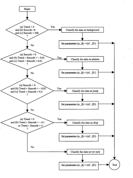
It is not guarantee that this model is the best choice, but any results and findings from this model can help to explore other time series model in the further studies.

The linear exponential smoothing model is modified before trying to fit it to the tab-chart. The modified model has the variable (dynamic) parameters, a and

p,

and a threshold value, T. In the fitting process, if the trend estimate of the model exceeds the threshold value, the variable parameters will take values al and

Pl.

Otherwise, they will take another values a2 and

p2.

The reason of using this policy is based on the difference of slope between significant signal changes (i.e. background and plateau) and flat parts (i.e. jump and drop). The parameters and the threshold value are adjusted manually until the model is fitted well to the tab-chart. After fitting the model to all tab-charts, it discovered that the threshold value T is more influential and important in finding the well-fitted model than the two parameters a and

p.

Besides, the fitted curve of the model is spiky when the threshold value is small but becomes smooth when the value gets larger. There is a remark that the above parameters policy is only an initial trial and not perfect, the experiment result will reflect and reveal what is the drawback and disadvantage.

For convenience, henceforth HOLT model is named for the above modified linear smoothing model. The first algorithm of detecting the point change (or time series segmentation) by HOLT model is called classification method. The main idea of the algorithm is explained at the following. The change of the variable parameters (i.e. a and

p)

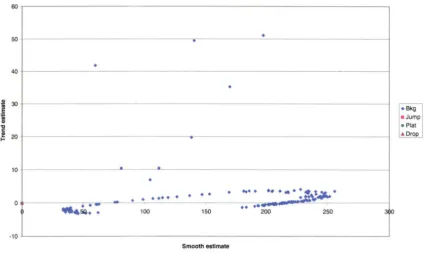
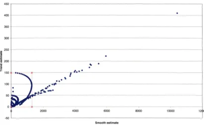
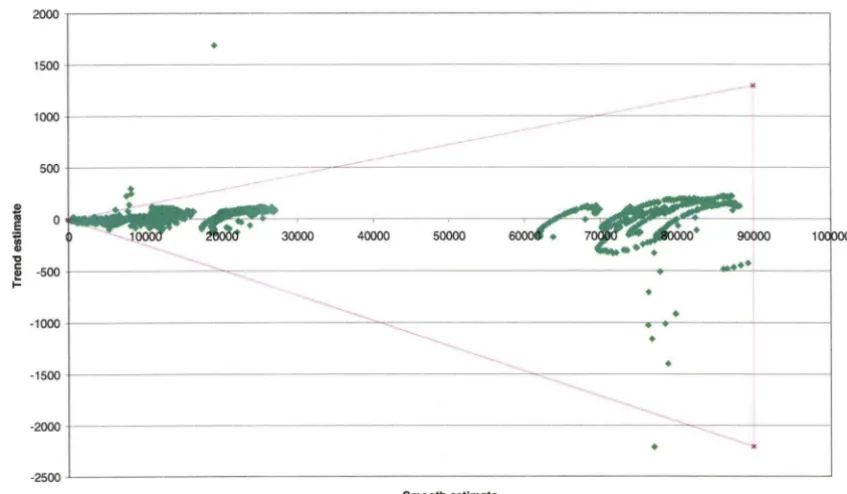
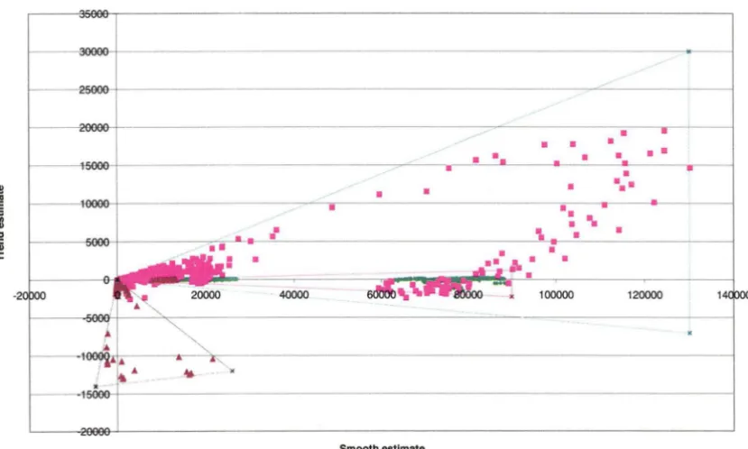
indicates the stage change in the tab-chart (i.e. from significant signal change to flat part or vice versa). For example, the values of parameters change from (al, PI) to (a2, P2) as the tab-chart moves from background (stage) to jump (stage) in standard sample. This classification method is not practical for the researchers and not automatic because it needs the human adjustment of parameters beforehand. However, this method has two purposes. Firstly, this method is a way to develop another automatic classification method. Secondly, this method is used as a tool to analysis the data reduction and fitted error of HOLT model.

(7)

trend-smooth graphs. The jump stage of the tab-chart has larger trend and trend-smooth values. The plateau stage of the tab has larger smooth values but small trend values. The drop stage of the tab-chart has negative and large trend values. The performance of the classification rules are verified and tested by applying to the tab-charts of standard samples. Some guidelines of evaluating the performance are made to minimize the personal and biased judgement. Different person possibly has different judgement and view on some borderline cases. The classification rules have the successful rate ranging from 45% to 80% in various elements. However, after excluding the tab-charts of having close background and plateau, the successful rate of the classification rates will be at least 65%. This project provides the good method and platform of identifying the point change. One promising way of improving the performance is to refine and modify the rules. Although the rules seem to play more important role in the performance than the parameters (i.e. a and ~). an experiment should be carried out to investigate any effect of the parameters on the performance.

For both classification method and rules, there is a problem of misclassification. This problem is that the classification and rules have the terrible performance in some tab-charts. In other words, there are a lot of observations in these tab-charts being wrongly classified. However, all these tab- . charts have the property that the level of background and plateau are very close. Thus, this is possibly the cause of misclassification but the gentle signal change (i.e. jump or drop having gentle slope) is another possible cause. Anyway, this problem gives us a hint to improve the performance of both method and rules. For example, another set of rules is needed to tackle these tab-charts. Besides, classification method is better than classification rules because rules are hardly to replace the human visual judgement. However, classification rules are automatic and more practical than classification method.

(8)

parameters. In other words, the background (or plateau of small signal) should use different a and ~

parameters.

After fitting the time series model to the raw data, the analysis of the fitted error should also be provided. From the analysis result, the fitted error of HOLT model increases as the level of plateau increases. The fitted error of the model decreases as the mass of the element increases. It is because the amount of heavy elements is smaller than the amount of light elements in the sample. Therefore, the only factor of affecting the fitted error is the level of plateau. This result implies that the standard deviation of fitting error of element's concentration can be minimized if the background noise can be controlled or minimized. Thus, the control of background noise can help to estimate the trace of the element in the sample more accurate but it is not capable of delivering only significant improvement to the major element in the sample.

For a comprehensive analysis, ARIMA model should also be fitted to the tab-chart. Since there are a lot of tab-charts to be fitted, a policy is devised to speed up the ARIMA model fitting. The procedures of fitting the ARIMA have the following three steps. The first step is to check the tab-chart is stationary. If it is not stationary, differencing will be carried out on the background of the tab-chart. The second step is fit AR(l), AR(2), MA(l), MA(2) and ARMA(l,1) to the background, the best model is chosen by the lowest MSE and significant parameters. If the five models cannot be fitted to the background, it may be random walk or has another ARIMA model. The third step is to use the above two steps to fit the ARIMA to the plateau of the tab-chart. After the model fitting, the result is obtained at the following. Over the background, no differencing is needed and most of the tab-charts are ARMA(l,l), random walk or inconclusive. Over the plateau, most of the plateaus having upward or downward trend are ARIMA(0,1,1), whereas most of the plateaus having horizontal trend are AR(l) or ARMA(l,1). The other plateaus are random walk or inconclusive. The above result also indicates that most of the tab-charts have the autocorrelation problem.

(9)

There are some inadequate places in this project and more work is needed on these places in further studies. Firstly, the classification rules are relatively approximated and should be refined. More advanced mathematical techniques could be employed to devise better classification rules. Secondly, the other models should also be explored and investigated such that they have better performance in change point detection and the researchers can gain more information from the tab-chart via these models, for example, locally weighted regression. Thirdly, this project does not have enough work on studying the parameters of the HOLT model. One way is to investigate the impact of parameters on the performance of classification rules because only one set of parameters is used in this analysis. Another way is to investigate the relationship between parameters and data reduction because the data reduction does not work on the background or plateau of small signal. Lastly, some studies should be done to tackle the tab-chart having the autocorrelation and influence of autocorrelation on the statistical estimate on the tab-chart by HOLT model.

Moreover, there are several directions worthwhile to be considered in the long-term goal. Firstly, the classification rules can be extended and applied to the tab-chart of multiple significant signals (i.e. jumps and drops) and multiple flat parts (i.e. backgrounds and plateaus). Secondly, when studying the standard samples in this project, the tab-chart of each element in a sample is investigated independently and separately. However, the mineral in the real sample is a chemical compound of elements. Therefore, the change of composition in real samples will involve the investigation of more than one tab-chart. Thirdly, the knowledge (i.e. model and method) of this thesis is not limited only on the composition investigation of minerals or rock samples. It can be generalized and applied to other areas (i.e. charts in other problem). Lastly, the HOLT model and other methods of change point analysis should be compared, especially their performances. Since the data reduction of HOLT model is to trace the trend of the tab-chart and remove the variation or noise, the HOLT model may be incorporate into other methods to get better performance.

HOLT model PIP, CUSUM etc

(Raw) time series Trend ofume series Change points found

(10)

Chapter 1 Introduction And Overview

(1.1) Preamble

Laser ablation - inductively coupled plasma - mass spectrometry (LA-ICP-MS) is a relatively new advance in instrumental multi-element low-level analysis that has been largely developed for geological research purposes, but is finding wider application to the in situ inorganic analysis of many solid materials [22], [23].

The LA-ICP-MS is a method to analyse the composition of minerals and the tab-charts will be produced from the ICP-MS instruments, which show the distribution and amount of elements in the mineral (see Section 1.8). In this research, the data reduction technique is applied to filter out the noise of the tab-charts and trace the trend of the tab-charts.

(1.2) Structure Of This Thesis

The first four chapters (i.e. Chapter 1 to Chapter 4) are informative and instructive. These chapters give the basic background information to the readers and help them to understand the work of this project in later four chapters (i.e. Chapter 5 to Chapter 8). The content in the first four chapters and Appendix A mainly come mainly from an unpublished paper [9], and additional materials (including paperwork and Excel spreadsheet) provided by CODES and the School of Earth Sciences, University of Tasmania and websites [16], [25] and [26]. These materials have been synthesised and rewritten for thesis presentation.

(1.3) Laser Ablation-Inductively Coupled Plasma-Mass Spectrometry

Laser ablation-inductively coupled plasma-mass spectrometry (LA-ICP-MS) is a new technique for measuring the inorganic composition of the minerals and other types of solid samples [16]. The CODES instrument has some special features [16], [25] which include (a) small amount of samples is sufficient and required for fully composition analysis; (b) the instrument can tackle very small-sized and any solid samples; (c) up to sixty elements can be analysed at one time; (d) the trace elements in the sample can be quantified and measured; (e) in some cases, heavier isotopes can be measured with good precision.

(15)

Chapter 1 Introduction And Ovef1!iew

(1.4) Laser Ablation Process

(LA)

Laser ablation is a process of using a laser beam to detach material from a solid sample. The ablated material is transported in an Ar gas stream to the torch of an ICP-MS for compositional analysis [9], [16], [25], [26]. Details of this process will be discussed later (see Section 1.6).

(1.5) Application OfLA-ICP-MS

LA-ICP-MS has wider application in both academic and industrial areas [16], [25]. They include (a) the evidence collection of crime and forensics; (b) elemental analysis and quantification of mineral and rock samples; ( c) the investigation of environment pollution; ( d) the exploration of the trace elements in polymeric materials; (e) process and quality control; (f) reliability and failure analysis.

In CODES (ARC Centre of Excellence in Ore Deposits) and the School of Earth Sciences at the University of Tasmania, the staff and other researchers have been routinely analysing sulphide and, to a lesser extent, non-sulphide minerals for minor and trace elements by LA-ICP-MS for several years. The technique allows for the quantitative measurement of up to 60 elements in situ with a spatial resolution of a few tens of microns, or less. Further details of the instrumentation are discussed in Chapter2.

(1.6) Two Types Of ICP-MS: LA Vs Solution

Before discussing the specifics of the CODES LA-ICP-MS instrument it is worth comparing LA- sampling with conventional (solution-based) techniques for presenting material to the ICPMS.

In LA analysis the material to be analyzed comprises very small particles with a range of sizes that are carried in a stream of Ar gas to the plasma of an ICPMS. In the plasma these particles are vaporized and ionized (see Section 2.3.1). Then the ionized species or ions are sampled and pass through a quadrupole mass discriminator (see Section 2.3.2) and on to a detector for counting. The detector measures the number of electrons I hits from the selected ions (see Section 2.3.3). Lastly, these numerical data are captured as a csv file for subsequent processing (see Section 4 .1).

For solution-based ('conventional') ICP-MS analysis the material being analysed is digested (dissolved) and presented to the plasma in a dilute, weakly acid, solution.

(16)

Chapter 1 Introduction And Overview

n:;;)

Lt::::=~

=La=ser (L=A>

===!I

I

Conventional Solution

Fig 1.6 (1) : LA-ICP-MS And Conventional Solution-ICP-MS. The input is sample collected from field site. whereas the output is data table

ICP-MS

(..___Ion___,s

I

ic=:=~

=Plasma

=:::::3

1 ic=:=~

D=etector=:::::3

1

. _ _ _ I _ _ _ _ . .

Fig 1.6 (2) The Internal Structure OUCP-MS. The output is spreadsheet

(

1. 7) A

dvantages Of LA-ICP-MS Over Con

v

entional ICP-MS

LA-ICP-MS has some advantages compared with conventional solution-ICP-MS [16], [25]. Primarily, the excellent spatial resolution (see section 2.2) allows sampling and analysis of complex microscopic intergrowths common to many geological materials. Sampling can be done in real time, and sample preparation is minimal (usually a polished piece of rock is used). Lastly, contamination is usually not a problem with LA techniques.

By contrast, solution techniques require much larger amounts of material (rock or mineral powder). The powders need to be obtained by micro-drilling, or sub-sampling a larger crushed rock sample. Both procedures may lead to sample contamination, either from adjacent mineral grains in the case of drilling, or from crushing equipment with larger samples. Furthermore, some types of

(17)

geological materials are notoriously difficult to dissolve in mineral acids, thus incomplete digestion can

also be a major problem with solution-based techniques.

(1.8)

Data From The ICP-MS: The Tab-Chart

A tab-chart (e.g., Fig 1.8) is a time-series graphical representation of all measurements made

by the ICP-MS instrument during the course of a single laser 'burn'. The x-axis represents the starting time of each cycle (see section 4.1), whereas the y-axis represents the counts per second or signal

intensity (i.e. counts for a particular ion as measured by the detector of the ICP-MS). Initially, counts are low (''background") until the laser is switched on. Laser switch-on is reflected in the tab-chart by an

abrupt increase in total counts for the elements of interest. The curves reveal an element's change as

the instrument is applying the laser on the sample (see Section 4.2.1). Tab-charts obtained for

'unknown'-samples are then compared to tab-charts for 'known' materials (referred to as 'standards')

in order to quantify individual trace elements in the 'unknown' sample being analysed (see Section

4.2.2, 4.2.3 and 4.2.4).

f

_c

i

;; c

"'

(;;

,,

c 0

:

;

"'

€

"

0 0 1000000 100000 10000

laser is off

1000

100

10

background signal

Tab-Chart Of Primary Standard

laser is on

sample from the surface

plateau signal

sample from the bottom

....,__. laser is off l+,.,.,m-n'l'TTTTTTTrn""rMTM'TrnmTITTTTTTTTMTM'TTTTTTIT"1'Tirm">'TTTTTTTTMTM'TTTTTTITTTTl'TTTnm"MTmTTTTTTTTMTM'TTTT'TTTT'TTTTTTTr,,.,,.,mTI'l'TTTn-ri

~~~~~~A~~~~~~.~~~~~~~~~~~~~~~~~

~~~~~~~~~~r~,~~~~~~~~~·#~~~

Time (soc)

Fig 1.8 : Tab-chart OfA Primarv Standard

Page4

- Ca43 - Sc45 T147 V51 - Ni60 - Cu65 - Zn66 - Rb85 Sr88 Y89 Zr90 Nb93 Ba137 La139 Ce140

Nd146

- Sm147 Eu153 Gd157 Dy163

- Er166

(18)

(1.9) Standard Samples Studied In This Project

This thesis deals with LA-ICP-MS data obtained from two 'standard' glass materials. The first

of these is a synthetic glass 'NIST 612' purchased from the US National Institute of Standards and

Technology. This glass has been doped with sixty-one trace elements to a nominal concentration of 50

mg/kg for each trace element. The second is a glass was produced in the School of Earth Sciences by

fusing a certified natural rock (basalt) powder (BCR2) sourced from the US Geological Survey. Over

the last couple of decades both NIST 612 and BCR2 have been extensively analysed in many

laboratories worldwide using many techniques. Hence, their composition is very precisely and

accurately known for a large number of elements. CODES provided the raw data from sixty-six

LA-ICP-MS spot analyses of these glasses (six of NIST 612 and sixty ofBCR2).

For the purpose of quantification of LA-ICP-MS analyses, unknown samples are usually

compared to a analyses of known materials such as NIST 612 and BCR2. These 'primary standards'

are analysed at regular intervals along with the unknowns (typically, two spot analyses of a primary

standard for every ten to fifteen unknowns). As well as quantification of unknowns, the regular analysis of primary standards allows instrumental drift to be accounted for during daily ICP operation.

Sometimes more than one 'known' is run with a group of unknowns, and the second known

('secondary standard') becomes an additional check on analytical precision and accuracy. For more

description and discussion on standard samples, see chapter 3.

(1.10) The Aims And Goals Of This Project

(1.10.1) The Main Aim And Goal

To date researchers identify and classify individual tab-charts by their observation, knowledge

and past _experience. This can be referred to as the 'visual' or 'intuitive' method. However there are

grey areas that they are not easy to identify and classify by simply observation. Therefore, it would_ be

useful to have some mathematical and statistical methods to aid with these judgements.

The main goal of the research described here is to find out systematic methods or rules to

classify tab-charts into different portions. Ultimately, this may aid geological researchers by allowing

tab-chart classification to be performed more quickly and automatically. The detailed work to this goal

will be presented in chapters 5 and 6.

(19)

Chapter I introduction And Overview

(1.10.2) The Other Aims And Goals

Apart from tab-chart classification, the researchers want to retrieve useful information from

the tab-chart quickly and automatically. Chapters 5 and 6 will provide the knowledge (including

equations and examples) how to get the information (i.e. statistical summaries) from the tab-chart.

Chapter 7 includes the quantitative and statistical analysis to validate the method and model and

evaluate their performance. This chapter also includes some work investigating factors affecting the

magnitude of errors. Chapter 8 investigates the autocorrelation structure of the tab-charts and fits and

criticize ARIMA models for the tab-chart segments.

(1.10.3) The Summary Of The Work In This Project

The work reported here concentrates on the data from the two glasses discussed in section 1.9,

with NIST 612 referred to as a 'primary standard' and BCR2 as a 'secondary standard'. Tab-charts for

'unknown' samples are invariably more complex than those of glasses, and their statistical analysis is

beyond the scope of the present study. The work of chapter 5 to chapter 6 is to find out the systematic

methods or rules and give their statistical summaries (see sections 1.10. l and 1.10.2). There are several

works shown in chapter 7. Firstly, the noise of the tab-chart and our method will be estimated.

Secondly, the error of our method will be estimated. Thirdly, the current method used by the

researchers and our method developed in this project will be compared. In chapter 8, the ARIMA

model will be applied to the tab-charts and some discussions are made about ARIMA model and our

method. The summary of chapter 5 to chapter 8 is displayed at the following graph.

Chapter 5

• Find the suitable time series to tab-chart

• Fit time series HOLT to the tab-chart

Chapter 7

• Evaluate the performance of HOLT

• Compare intuition method and HOLT

Chapter 6

• Find the rules of classifying the tab-chart

• Evaluate the performance of the rules

•Discuss the limitation of the rules

Chapter 8

• Fit ARJMA model to the tab-chart

•Compare HOLT and ARIMA model

Fig I.JO : Summarv OfChaoter 5 to Chapter 8

(20)

(1.11) Literatures (Current Methods And Our

New

Method)

(1.11.1) Literatures OfLaser Ablation Process

The materials and information about laser ablation process can be referenced to [9], [22], [23], [25], [26] and [27]. The work of this project is based on the paper [9] and the raw data is provided by CODES and the School of Earth Sciences, University of Tasmania.

(1.11.2) Literatures Of Change Point Analvsis

Change point analysis (detection) or time series segmentation is a problem in the data mining and this problem has two directions : the first direction is to detect the mean shifts in the time series and the second direction is to detect the variance change in the time series. For simplicity, the problem is how to divide (cut) a time series into segments. Each segment represents a mean shift in the time series. Change point analysis is familiar with statistical process control (SPC), which is used to · monitor the process and detects any occurrence of out of control and abnormal pattern. SPC is well-known in quality and process control. The main difference between SPC and change point analysis is that the former focus on the detection of change point one at a time but the latter detects all change points at one time.

P. Hubert (2000) shows that the change points (mean shifts) in the time series can be modelled as a tree. The change points are found by choosing the segmentation in the least squares sense. The solution space is huge and branch and bound is impossible to tackle for moderate sized problem. So this paper uses the Scheffe test and some constraints to find the solution. Fang Li (2006) tackles the change points (mean shifts) in multivariate process by tree-based supervised learner. Chen (2008) uses the evolutionary method to solve the problem of change points (mean shifts). In his journal, he uses k-means and Euclidean distance to calculate the fitness of chromosome.

Taylor (2000) uses cumulative sums of difference (CUSUM) and bootstrapping to detect the change points (mean shift and variance change) in the time series. The idea is that a change in direction of the CUSUM chart indicates a change point in time series. However it is not easy to identify the change points by observing the CUSUM chart only. Thus, bootstrapping produces the bootstrap CUSUM charts to help to find out the change points. This method can be applied to both mean shift and variance change problem. Carslaw (2006) is a paper to apply the technique CUSUM and , bootstrapping to urban air pollution concentration time series.

Fu (2006) uses perceptually important points (PIP), a method is applied to technical patterns in finance and stock market, to identify the change points (mean shift) in the time series. The time series is re-arranged into their importance by PIP identification process. The most important point is

(21)

the first change point and the second important point is the second change point in the tine series and so on. Then a binary tree is constructed and the change points are retrieved from the tree according to their importance. Kumar (2001) incorporate fuzzy set theory into the change point analysis. This article states that the change point (mean shift) often occur over a time interval and should not be treated as a sudden change at a particular time.

The linear Holt exponential smoothing model is chosen in this paper and applied to the tab-chart. Since the tab-chart is actually a time series, the useful signal and information can be reflected and extracted by fitting the model to the tab-chart. In this thesis, this model is modified and can be used to divide the tab-chart into different segment. Comparing with the other methods of change point analysis, the modified model has two advantages. Firstly it is easily implemented in the Excel spreadsheet. Secondly, apart from the function of change point detection (i.e. time series segmentation), the modified model can also provides the statistical information (summaries) and estimate error of each segment. The model is also capable of removing the variation and noise from the tab-chart. Thus, the researchers can gain the useful and comprehensive information in the fast and efficient way.

The modified model is applied to the standard sample in this thesis because it is artificial and made in the laboratory. The situation becomes more complicated in the real samples. However, the study of standard samples can build the good foundation and platform for studying real samples. It

offers the prospect of building up knowledge about tab-chart and understanding the advantages and disadvantages of the modified model.

(22)

Chapter 2 Laser Ablation Process And Machine Description

Chapter 2 Structure OfLA-ICP-MS Instrument

(2.1) CODES Laser Analytical Facility

The CODES Centre of Excellence in Ore Deposits at the University of Tasmania operates a

laboratory equipped with laser sampling (Nu Wave UP-213) and ICP-MS (Agilent Technologies 4500

plus) instruments, which are used to analyse the composition ofrock and mineral samples. This chapter

briefly describes these instruments and their operation.

(2.2) Nu Wave UP-213 Laser Ablation System

This part of the system (Fig. 2.2 (1) and Fig 2.2 (2)) allows careful targeting with high spatial

resolution of small areas of (polished) rock and mineral samples. The sample chamber accommodates a

single 2.5 cm diameter polished mount that can contain unknown samples or standards. A video camera

and microscope allow real-time imaging of the mount and laser ablation run. A computer-controlled,

motorized X-Y-Z stage allows precise movement (± few microns) of the sample to allow selection of

laser targets. The laser software (MEOLaser-213) controls the laser parameters including spot size,

laser energy, pulse rate and firing of the laser and ablation takes place under a stream of He gas that

carries the ablated material away and towards the ICP-MS.

Fig 2.2 (1) : UP-213 Laser Ablation System

(23)

Fig 2.2 (2) : Sample Chamber And Motorised Stage

(2.2.1) The Function OfLaser and Gas

The laser is pulsed and interacts with the surface of the rock sample. In a complex process, partly dependent on the nature of the sample, tiny amounts of material are ablated and a hole is created. He and Ar gas carry the ablated material to the plasma of the machine ICP-MS. There are two types of laser operation on the rock sample : spot (vertical) analysis and line analysis.

laser melted sample He or Ar gas

Step 1 : Laser hit the sample sur(ace Step 2 : Sample is melted Step 3 : He gas entrain the sample

Fig 2.2 (3) The Job Of laser And Gas In Sample Chamber

(2.2.2) Spot (Vertical) Analysis

In spot mode the laser can produce a hole ranging from 8 to 110µ.m in diameter. The laser is pulsed (5 to 10 Hz) and continues to hit on the same spot during the process. However, as the hole deepens (typically 10 to 30 µm, it becomes more difficult for the carrier gas to entrain material from the bottom of the hole. This will cause the decrease in the signal intensity. Spot analysis allows for easy removal of surface contamination by pre-ablating the spot for a few cycles of the laser.

(24)

Chapter2 Laser Ablation Process And Machine Description

(2.2.3) Line Analvsis

In line analysis, sample is moved beneath the laser as analysis proceeds. This produces a

shallow linear sampling track across the sample, instead of a single hole. Dealing with surface

contamination in line analysis can be problematic.

(25)

Chapter-2 Laser Ablation Process And Machine Description

(2.3)

Agilent

HP4500plus Quadrupole

· ICP-MS

The ICP-MS instrument is responsible for analysing the composition of ablated material. It is

made up of three main parts: plasma, mass discriminator and detector. In detail, a silica glass torch and

induction coil produces an Ar plasma when the instrument is running; twin metal cones with

'pinholes', just beyond the plasma, allow ions to pass into the second (high vacuum) part of the

instrument which is a quadrupole mass filter (Fig. 2.3 (3)); and ions selected by the quadrupole filter

are then counted by an electron multiplier device that can operate in both pulse (for low count rates)

and analog (high count rate) modes. Numerical data from the detector are tabulated by the ICP-MS

controlling software as csv tables suitable for export to Excel or other software packages.

Fig 2.3 (/) : Mass Spectrometer I ICP-MS

(2.3.1) ICP Torch Body/ Plasma

The ICP torch body three concentric silica glass tubes wrapped by an induction coil. The coil

is used to transmit radio frequency energy to the Ar gas flowing through the three tubes (Fig 2.3 (2)).

The plasma in the central (injector) tube of the torch may reach temperatures of over 6500"K.. Such a

plasma is very efficient at breaking chemical bonds and creating simple (singley-charged) ionised

species.

(26)

quurtt tutrn~ and

L

A•rosol sample

Fig 2.3 (2) : Plasma (Source From http://ewr.cee. vt.edulenvironmentallteach/smprimer/icpmslicpms.htm)

(2.3.2) Mass Discriminator Or Ouadrupole Mass Filter

Mass discriminator or Quadrupole mass filter is a vacuum chamber. This vacuum environment

prevents the collisions between ionised species and air molecules. This chamber contains four magnetic

rods ('quadrupole'), which is used to select the specific ionised species for detection. By changing the

intensity of magnetic field, only selected species will reach the detector on other side of the chamber,

whereas other species are driven away from the chamber based on their mass to charge ratio.

Fig 2.3 (3) : Mass Filter (Source From http://ewr.cee. vt.edulenvironmenta/lteach/smprimerlicpmslicpms.htm)

(27)

(2.3.3) Detector

The detector is an electron multiplier (Fig. 2.3 (4) and (5)) and the last major component in the

machine ICP-MS. Positive ions reaching the detector are attracted to it and release electrons when they

impact the first part of the detector, these in turn impact the next .Part of the detector to produce more

electrons. This 'multiplier effect' helps account for the high sensitivity ofICP-MS analysis.

Fig 2.3 (4) : Detector (Source From http://minerals.cr.usgs.gov/icpms/intro.html)

Anillog

- ;

~,..,.,. • _,_ M,..,,. • l •T" ~ I• (? t' j { I <f 1

ii-. .. • ,.,.,,.,.

Fig 2.3 (5) : Detector (Source From http://www.uea.ac.uklenv/technical/lab/icp-ms2.shtmll

(28)

Chapter2 Laser Ablation Process And Machine Description

(2.3.4) Sample Composition Investigation

In combination, the quadrupole mass filter and the detector rapidly scan the isotope masses being measured (- 0.5 seconds to scan and count 30 different masses). Counts are accumulated for each mass and recorded. In a typical LA analysis ablation and counting would continue for about 100 seconds, generating more than 150 scans across the mass spectrum (there is time 'lost' while the detector is inactive between scans). Data for each selected mass is captured as counts per second (cps) for each scan. These machine generated data tables form the basis for all subsequent calculations and quantification ofLA-ICP-MS data.

Start

The first cycle of measurement start

Sent all signals (i.e. cps) to MS Excel

Start a new cycle of measurement

Yes

Proceed to next element by adjusting magnetic field in mass discriminator

Detector measured number of electrons I hits from the chosen element

ICP-MS convert number of electrons I hits into count per second (cps)

Detector has a short period of inactivity

Fig 2.3 (6) : Detector Job In ICP-MS Machine

(29)

Chapter3 Materials Used

Chapter 3 Materials Used For This Study

(3.1) Standards

Quantification of ICP-MS analyses is made by comparing measurements made on unknown materials to measurements made on well (compositionally) characterised natural or artificial materials under similar analytical conditions. These 'known' materials are referred to as standards. For solution-based ICP-MS the standards are solutions made to contain precisely known concentrations of the elements of interest. For LA-ICP-MS standards are either synthetic glasses 'doped' with a variety of trace elements, or natural materials fused to a homogeneous glass. In the latter case, the composition of the glass has been agreed by multiple-interlab and multiple-instrument procedures. Glasses make good LA-ICP-MS standards because, at the scale of laser sampling, they are homogenous and trace elements are assumed to be uniformly distributed.

For the work undertaken herein LA-ICP-MS data from two glass standards (NIST610 and BCR-2) have been used. NIST610 is a synthetic silicate glass doped with a nominal 50 ppm of 61 elements prepared by the US National Institute of Standards and Technology (www.nist.gov) and Fig 3.1 (1). BCR-2 is a basalt powder prepared by the US Geological Survey (minerals.cr.usgs.gov/geo_chem_stand/basaltbcr2) - Fig. 3.1 (2). A small aliquot ofBCR-2 was fused in a platinum crucible and quenched to an homogenous glass at the laboratory at the School of Earth Sciences, University of Tasmania.

(3.2) Primary Vs Secondary Standards

For quantification purposes (see Chapter 4), the standard used to calculate elemental concentrations in LA-ICP-MS analysis is referred to as the 'primary' standard. Sometimes, in order to check analytical precision and accuracy during routine LA-ICP-MS runs, another glass standard is analysed and treated as an 'unknown'. This second glass standard is referred to as a 'secondary' standard.

Primary standards are analysed before and after the analysis of unknown samples (pre- and post-analysis). Commonly, two measurements of the standard glass bracket each set of 10-12 unknowns. By bracketing measurements it is possible to correct for machine drift (see Chapter 4).

The CODES and the School of Earth Sciences provides sixty-six standards to this project. Six standards are primary standards (samples 1, 2, 33, 34, 65 and 66) and the other samples are secondary standards. There are twenty-eight elements in each standard. Therefore there are total 1848 (= 66 samples x 28 elements in each sample) tab-charts for the studies in this project.

(30)

Chapter 3 Materials Used

Fig 3.2 (I) : Composition of Standard Glass -NIST6! 2. Corrected to six significant figures

41.54 0.000077 0 0

37. 73 0.000070 0 0

34.73 0.000065 0 0

98740.5 0.184184 21.92 0.000041

13.31 0.000025 28.32 0.000053

77.44 0.000144 42.93 0.000080

0.012843 0.000000 37.96 0.000071

10531.6 0.019645 38.34 0.000072

1.99 0.000004 0 0

339876 0.633984 41.64 0.000078

72.72 0.000136 37.74 0.000070

55.16 0.000103 35.77 0.000067

66.26 0.000124 38.35 0.000072

0.007982 0 37.16 0.000069

84691 0.157978 35.24 0.000066

11.85 0.000022 36.72 0.000068

41.05 0.000077 34.44 0.000064

48.11 0.000090 36.95 0.000069

0.008022 0.000000 35.92 0.000067

39.22 0.000073 35.97 0.000067

39.88 0.000074 37.87 0.000071

38.43 0.000072 37.43 0.000070

56.33 0.000!05 37.55 0.000070

0.007247 0.000000 39.95 0.000075

35.26 0.000066 37.71 0.000070

38.44 0.000072 34.77 0.000065

36. 71 0.000068 39. 77 0.000074

37.92 0.000071 39.55 0.000074

36.24 0.000068 8.12 0.000015

34.64 0.000065 0 0

37.33 0.000070 0 0

14.44 0.000027 5.09 0.000009

31.63 0.000059 15.07 0.000028

76.15 0.000142 38.96 0.000073

38.25 0.000071 29.84 0.000056

35.99 0.000067 37.23 0.000069

38.06 0.000071 37.15 0.000069

38.3 0.000071

(31)

Chapter 3 Materials Used

Fig 3.2 (2) : Composition o[Standard Glass BCR-2. Corrected to six significant figures

'6~'11 ' '111''' , ':

9.20 0.000017 0 0

2.30 0.000004 0 0

0 0 0 0

23603.3 0.042895 0 0

3.18167 0.000006 0 0

22249.9 0.040435 0 0

3.69 0.000007 2.5 0.000005

71948.4 0.130754 0.28 0.000001

13.595 0.000025 0 0

251441 0.456950 1.17 0.000002

53. 7983 0.000098 682 0.001239

1608.22 0.002923 25 0.000045

14721.3 0.026753 53.7 0.000098

1.77333 0.000003 6.78 0.000012

50957.6 0.092607 28.6 0.000052

7.13 0.000013 6.6 0.000012

32.6 0.000059 1.95 0.000004

13434.4 0.024415 6.68 0.000012

2.24 0.000004 1.05 0.000002

413 0.000751 6.3 0.0000/l

14. 7 0.000027 1.28 0.000002

1548.91 0.002815 3.61 0.000007

96249.6 0.174915 0 0

12.3822 0.000023 3.38 0.000006

39 0.000071 0.5 0.000001

12. / 0.000022 4.9 0.000009

23 0.000042 0.81 0.000001

125 0.000227 0 0

22 0.000040 0 0

0 0 0 0

46.8 0.000085 0.29 0.000001

333 0.000605 JO 0.000018

33.4 0.000061 0 0

183 0.000333 6.05 0.0000/l

12 0.000022 I. 7 0.000003

244 0.000443

(32)

Chapter3 Materials Used

(3.3)

Internal Standards

During the course of each individual (standards and unknowns) measurement (usually 60-100 seconds) systematic variations in signal intensity can occur for several reasons unrelated to 'real' changes in the composition of the material being analysed. For quantitative ICP-MS analysis, an 'internal standard' is used to account for these fluctuations. An internal standard can be any constituent of the material being analysed for which accurate independent compositional information is available. For solution ICP-MS analysis of solutions, internal standards are usually one or more elements added to the solution in known amounts. For LA-ICPMS the internal standard element is usually a major element of the mineral being analysed previously measured by electron microprobe or by assuming mineral stoichiometry. For example, elements Fe and S are the internal standard elements used in pyrite analysis, whereas elements Pb is the internal standard elements for galena.

(33)

Chapter4 Tab-chart And Ca/culatwns

Chapter 4 Tab-Charts And Calculations

(4.1) Raw Data

The ICP-MS detector measures the raw data of signal I counts per second (cps) for one isotope at a time, with the mass spectrometer rapidly cycling through a pre-selected list of isotopes (elements). This means a single laser run of 60 to 80 seconds produces numerous short counts for each isotope. Counting takes place while the detector 'dwells' on each selected isotope (typically 20-30 milliseconds, depending on the number of isotopes selected). There is a 'settling' time of a few milliseconds between each mass jump. The ICP-MS software preserves the counts and some other instrument parameters as csv data tables which are imported into Microsoft Excel for further manipulation. There are three uses for these data sheets : plotting 'tab-charts', calculating element concentrations and calculating analytical error [9].

Figure 4.1 (1) and (2) has examples of these csv tables presented as an Excel spreadsheet. Due to the limited space, only small portion of two spreadsheets, containing )he raw data of secondary sample 25 and 12, are shown in the following graphs. Actually, there are total 29 columns and 149 rows in each spreadsheet because 146 cycles are done in the primary and secondary sample. The column represents the readings (i.e. cps) of an element in all cycles, whereas the row represents the readings (i.e. cps) of all elements in each measurement cycle. These readings are then used and plotted as the tab-chart (see Section 4.2.1).

By looking into the first spreadsheet at below, the row 4 represents the first measurement cycle. This cycle starts at time 0.624. The ICP-MS detector measures the cps of the elements in the sequence Ca43, Sc45, Ti47, V51, ... , U238. After this isotope finishes counting, the detector stops for a while (i.e. settling time). A second the second cycle (i.e. row 5) starts at time 1.237 and repeats the same measurement process. The last cycle occurs at time 89.576 and the measurements are recorded at row 149. For example, the ICP-MS detector measures that the cps ofV51 at measurement cycle 140 is "52311.19".

(34)

Chapter 4 Tab-chart And Calculations

A

8 c

D E

1 C:\DATA\050309\MA09C25. D File name and sample 25

2 Intensity Vs Time CPS

3 Time (Sec) Ca43 Sc45 Ti47 V51

...--

For each cycle, the machine

4 0.624 450 0 0 50 measures elements from left

5 1.237 250 0 0 0 to right one by one

6 1.85 450 ·O 0 0

~

The third cycle starts at time 1 .85

In this cycle, the machine measures ~ This cycle starts at time 85.899

k""" that the cps of V51 is "52311 .19"

143 85.899 11953.19 5250.61 130580.8 52311.19

144 86.512 11953.19 4800.51 135057.3 55619.17

145 87.126 10802.61 4050.37 132995 55769.54

146 87.739 10802.61 5550.69 126758.8 55869.79

147 88.353 11753.09 4250.4 128016 52762.25

148 88.966 10902.65 4300.41 128820.6 57323.47

149 89.576 11202.8 4350.42 126256 51208.64

Figure 4.1 (1) Raw Data Q(Sample 25 Compiled Jn Microsoft Excel

~~

@fie tdt !low II-' - !°"" l!ot• - tie<> ~~

Dr;i;liil,dl tl~::>' i~ <J _.

'"

"'

.

.,_ I: r- SUi ii J!__.e llXl'I<. - Ill.

"""'

- 10 B I II

., •,. m

c _-e.-~- ':" R39

A 8 c G H J:<_ _ L _ _ M N _L _~_P_--_~_:!:: 1 C:IDATA'll503'.l9\MAIJC1 2. 0

2 Intensity Y CPS

Srr

I

3 Time [Sec:ca43 Sc-45 r~7 V51 Ni60 C.£5 Zn66 Rb05 s.ee Y89 ldJ Nb93 Ba137 La139 Ce140 Nd146 4 0.624 500.01 100 100 0 50 50 0 250 0 0 0 0 0 50 50 0 5 1.237 550.01 0 0 0 0 350 0 50 0 0 0 0 50 0 0 0 6 1.85 350 150 0 0 0 50 50 50 0 50 0 0 0 50 0 0 7 2.464 500.01 0 50 50 0 50 100 50 100 0 0 0 50 0 0 0

8 3.078 550.01 100 0 50 0 150 50 100 0 0 0 0 50 0 0 0

9 3.691 150 100 0 0 0 50 0 0 0 0 0 50 0 0 0 0 10 4.304 400 0 0 100 0 250 50 150 0 0 50 0 50 0 0 0 11 4.918 600.Dl 100 50 150 0 150 50 200 0 0 0 0 0 0 0 0

12 5.532 400 0 50 0 0 100 0 150 0 0 0 0 0 0 0 0

13 6.145 500.01 0 100 0 0 100 50 50 0 0 0 0 0 0 0 0 14 6.758 500.01 50 50 0 0 100 0 250 0 0 0 0 0 0 0 0 15 7.372 300 50 50 50 0 100 0 150 0 0 0 0 0 0 0 0 16 7.985 450 0 0 50 50 50 50 150 0 0 0 0 0 0 0 0 17 8.599 550.01 100 0 50 0 50 0 50 0 0 0 0 0 0 50 0 18 9.212 350 50 50 0 0 0 0 150 0 0 0 0 0 0 0 0 19 9.826 250 150 0 50 0 50 0 50 0 0 0 0 0 0 50 0

20 10.439 350 0 50 0 0 150 0 100 0 0 0 0 0 0 50 0

21 11.053 450 50 0 150 0 0 0 50 0 0 50 0 0 0 50 0

22 11.666 300 200 0 0 0 150 50 200 50 0 0 0 0 0 0 0

23 12.28 500.01 0 0 0 0 100 0 100 0 0 0 100 50 0 0 0 24 12.893 300 0 0 0 0 100 0 200 0 0 0 0 50 0 0 0

25 13.507 450 0 100 50 0 200 50 100 0 0 0 50 0 0 0 0

26 14.12 550.01 250 0 0 50 0 0 150 0 0 0 0 0 0 0 0 27 14.734 450 50 0 50 0 50 0 100 0 0 0 50 0 0 0 0 28 15.347 400 100 0 50 0 150 50 0 0 50 0 0 0 0 0 0

~t 15.961 600.01 50 0 50 0 50 100 200 0 0 0 0 0 0 0 0 16.574 500.01 0 0 0 50 50 0 100 0 0 0 0 0 0 0 0

31 17.188 250 50 50 0 0 150 50 0 0 0 0 0 0 0 0 0

32 17.!ll1 400 100 0 50 0 50 150 50 0 0 0 50 0 0 0 0

33 18.415 550.01 50 50 0 0 50 100 50 0 0 0 0 0 0 0 0

34 19.028 200 0 0 100 50 50 0 50 0 0 0 0 0 0 0 0

35 19.642 350 150 50 0 0 100 0 50 0 0 0 50 0 0 0 0

36 20.255 350 150 0 0 50 100 0 50 0 0 50 0 0 0 0 50 37 20.869 550.01 150 0 200 50 50 0 150 0 0 0 0 0 0 0 0 38 21.482 400 150 50 100 0 200 0 0 0 0 0 0 0 0 0 0 39 22.096 350 150 0 0 0 150 50 100 0 0 0 0 50 0 0 0

"·-, • >i\-o;..,T\...ta/ --

-

-L~I -- _•_J

Figure 4.1 (2) Raw Data O[_Sam12,lg, 12 Compiled Jn Microsofl Excel

(35)

Chapter4 Tab-chart And Calculations

(4.2) Tab-Chart Description

(4.2.1) Structlire Of Tab-Chart

A 'tab-chart' is a graphical, time-series representation of all measurements made by the

ICP-MS instrument during the course of an individual spot or line analysis. Figure 4.2 (1) show a tab-chart

of primary standard. A single analysis usually takes 90 to 120 seconds, ~th the first 30 seconds used to

measure the background from the Ar and He carrier gas and the plasma. When the laser is switched on

ablated material is rapidly carried to the plasma. This causes a sudden jump to much higher count rates

for the elements being measured. Quite quickly, this signal stabilises to a flat pattern for the remainder

of the ablation, only dropping when the laser is switched off. These two parts of the tab-chart are

labelled jump and plateau on Figure 4.2 (1).

The plateau portion of tab-chart is used for concentration calculations. The plateau is

subdivided into one or more portions called integration interval. Each integration interval has

consistent trend or slope, assumed to represent homogenous phases or zones in the sample.

.f

!

_;; c

"'

iii :;; c 0

:

;

...

t1

"

0

0 1000000 100000 10000 1000 100 10

Tab-Chart Of Primary Standard

laser is on

laser is off

sample from the surface sample from the bottom

- Ca43 - Sc45

T147

V51 - Ni60

- Cu65

- Zn66

- Rb85

Sr88 Y89 Zr90

Nb93

Ba137

La139

Ce140

Nd146 +'-'f'-T<ifl-'-f!'--'rtttT;l-';---tr7'tl-ft-lr'l1~ftt--r'ri---t-~~~~~~~~~--r-~~~~~~~~~--'!rrh, - Sm147

plateau signal Eu153

Gd157

Dy163

I

Er166

la: : ; - Yb172 - lu175

1-trn'TTT'l"TTTTTTTTrn-nnTMTrrr"T'TT'TTTTT,,,,,'TTT'l"TTTTTTTTrn-nmTimTITn'TTTTTnTM"TTTTTTITnTT"mTITTTTTTTTn"TTinTM'TTT'ITTITTTTTnTT"'TTT'l'TTT'ITTITTTTI Hf178 - Ta181

#

~

'\-:}

<ft

~~ ~"-

&'

#

..._<3' p"-

4' #

.{ff ~";>

#' #

'\<9-'JI-{\

#' #'

#.c-.'ij' .... ~ ~;,

rf

A <p"- ":.{\

.#' ;,"-'), ;,'\;,

~":,~~~~~~~~~~~- ~·~.,~~~~~~~~~~~~

Time (sec)

Figure 4.2 (1) Tab-Chart Description

Page 22

- Pb208 - Th232

(36)

Chapter4 Tab-chart And Calculations

(4.2.2) Investigation O(Element Composition In Tab-chart

In natural heterogeneous materials the different zones can be identified by the trend and

change of signal in the tab-chart. If there is a change in the composition of major elements, it indicates

that another mineral has been reached in the sample. Figure 4.2 (2) shows an example of a single

analysis accidentally ablating two minerals in one 'burn'. The spot ablation commenced in pyrite (high

Fe but low Cu), then penetrated into chalcopyrite (increase in the signal from Cu).

10000000

1000000

~

..

i

100000

...

_c ₁₀₀₀₀

"'

iii :;;

c

0 1000 ¥

..

; 100 Q.

~

:J

0 ₁₀ u

integration interval

v

Fe Cu

pyrite chalcopyrhe

Time (sec)

Figure 4.2 (2) Tab-Chart O(A Sample Having Different Minerals (Source From (911

- 9

Ge72

As75 Se77

Zr90

Mo95

AQ107

C<!111

Sn118

- Sb121

Te125

80137

La139 W182

- Au197

- 205

By looking into tab-chart pattern, researchers can obtain a qualitative indication of the

proportion and distribution of various elements in unknown samples. Figure 4.2 (3) is a sample of

pyrite with generally flat and parallel patterns for the elements Pb208 and Bi209. This indicates fairly

evenly distributed micro-inclusions of galena (PbS) in the sample, or an even distribution of Pb and Bi

substituted in the pyrite lattice. By contrast, the very 'spiky' Pb and Bi in pyrite shown on Figure 4.2

( 4) indicate large discrete galena inclusions are present in the sample.

Geological workers currently identify the spikes and signals by visual inspection and

categorisation of the tab-charts. They need to decide these spikes and signals are caused by the mineral

inclusion, systematic changes in a mineral's composition or simply random noise or other unknown

reasons. Therefore, one of this project's aims is to find systematic and automatic methods to classify

these spikes and signals. One approach is to use the statistical methods I tests to test their significances.

If these spikes or signals are significant when challenged by these tests, we can conclude that they are

caused by the 'real' features of the material being analysed. Otherwise they are caused by random noise

or other unknown reasons and must be included in concentration calculations.

(37)

Chapter 4 Tab-chart And Calculations

10000000 integration hHarval - Ti49

.... - Cr53

Mn55

1000000 Fe57

- Co59

- Nl60

:G

_.,

- Cud5

100000

!

;; As75

c _Se77

"'

10000

-

--

· -

-

-(ii _Zt90

...

Mo95

c

0 Ag107

¥ 1000 Cd111

.,

~ Sn118

...

_- _SIJ1₂₁

.,

1: ₁₀₀ - e125

:I

0 83137

u

La139 W182

10

PIJ208 81209 - Tll232

- U238

Time (sec)

Figure 4.2 (3) Tab-Chart Of Pyrite Sample Having Evenly Distributed Micro-Inclusions Of Galena (Source

From {91) ~

..

c ! .5 ;; c

"'

(ii

...

_c 0

...

• .,

;

...

~ _:I 0

u

10CO:l0000

10000000

integration interval

----

· ==

-

=

---

-

~

-

----

---

--

1]

- 1149

- Cr53

Mn55

Fe57

- Co59

1000000

100000

10000

1000

< I ,

i,t~(

100

z:l

<

·

10

Figure 4.2 (4)

~

1i

Time (sec)

- Ni€0

- Cl.165 - Zn66 - Ge72 As75 Se77 Zt90 Mo95 Ag107

Cd111 sn11e

- Sb121

- e125

- 83137

La139

- W182

- Au197

- 205

- Pb208

-81209

- Th232

- U238

Tab-Chart Of Pyrite Sample Having Discrete Galena Inclusions (Source From {91)

Statistical methodology for tab charts : data reduction techniques in laser ablation analyses

Department Of Mathematics