Robotic Vision By Using Bee Algorithm

(1)

Robotic Vision

By Using Bee Algorithm

by

Liang Zhou

A dissertation submitted to the School of Computing

in partial fulfillment of the requirements for the degree of Master of Computing

(2)

Declaration

I hereby certify that this thesis contains no material which has been accepted for the award of any other degree or diploma in any tertiary institution, and that, to the best of

my knowledge and belief, this thesis contains no material previously published or written by another person except where due reference in made in the text of this thesis

Signed:__________________________________ Date:______________________

(3)

Abstract

With the development of technologies, robots have played an important role in many fields of the society. They help people to deal with a large amount of work, especially

operate in the extremely dangerous environment instead of people. For a robot, effective obstacle avoidance is still a challenge in the development of robot. The existing systems sometimes combine with multi-devices to conquer this challenge so that the expensive cost has been as a negative factor that cumbers the application of robot. For this purpose, find a way with the low equipment requirement but still having the high accuracy is essential. Optic flow as another algorithm coming from bee vision has been used to help robots avoid obstacles for many years. And it owns many advantages.

This study presents a system based on the optic flow is developed to avoid obstacle in

(4)

Acknowledgements

It was really a laborious task to accomplish a M.C thesis. Many people gave me support and helped in the process of writing this paper. Firstly, I would like to give

(5)

List of Figures

Figure 2 -1: The view-field of bees...4

Figure 2-2: The process flow of the obstacle avoidance system ...8

Figure 2-3: The results for the turning decision in the obstacle system...10

Figure 2-4: The Logitech Quick Camera ...12

Figure 3-1: The calibration image...19

Figure 3-2: The first step of the Install for OpenCV...20

Figure 3-3: The second step of the Install for OpenCV ...21

Figure 3-4: The third step of the Install for OpenCV...21

Figure 3-5: The paths configuration for OpenCV library under the Visual Studio 6.0 ...21

Figure 3-6: The first step of the paths configuration of OpenCV for a project...22

Figure 3-7: The second step of the paths configuration of OpenCV for a project ...22

Figure 3-8: The camera is connected to the laptop by using a single cable ...23

Figure 3-9: The scale in the experiment environment ...23

Figure 3-10: The background in the experiment environment ...24

Figure 3-11: The light condition in the experiment condition...24

Figure 3-12: The experiment environment...24

Figure 4-1: The absolute difference for the values of optic flow ...31

Figure 4-2: The camera was taken in a time...31

Figure 4-3: The camera was taken at another time ...32

Figure 4-4: The accuracy rates for both light conditions ...34

Figure 4-5: The accuracy rates for both circumstances: with calibration technique and without calibration technique ...36

(9)

(10)

List of Tables

Table 4-1: The values of the optic flow at the position: 0cm in the different time. ....30

Table 4-2: Results for the light condition: eight daylight lamps ...32

Table 4-3: Results for the light condition: four daylight lamps...33

Table 4-4: Results for the computation of optic flow without calibration technique ..34

Table 4-5: Results for the computation of optic flow with calibration technique ...35

Table 4-6: The values of the optic flow in two situations ...36

Table 4-7: The times for the image capture and the computation of the optic flow in the different place ...38

Table 4-8: The values of optic flow in this experiment 6 ...40

Table 4-9: The details of the computer used in this study...42

(11)

Chapter 1

Introduction:

Since the creation of the first robot in 1961, the field of robotics has undergone significant growth and development. One of its primary goals is to make robots operate independently. This has led to robots being built to carry out complex and extremely dangerous tasks without human supervision, and others that make human life and work more efficient such as automated driving robots and robots performing repetitive assembly line work. One important application area is autonomous robot

navigation and this has been developed along two separate fronts: vision-based navigation for indoor-robots and vision-based navigation for outdoor robots. As a general point in navigation, an automated robot should have three basic functionalities: perceiving, planning and acting so that it can gain information from an environment where it runs in, then analyze this information, and finally make an action on this environment. Vision systems provide a major source of information about a robot’s immediate environment and, thus, play an important role in the provision of autonomy. Guilherme (2002) stated that robotic navigation with vision systems can be divided into three categories: Map-Based Navigation, Map-Building-Based Navigation and Mapless Navigation. In the first two categories, two cameras are used as the main

(12)

In this work we will look at optic flow as a method of providing information for robot control. The hypothesis under examination is:

Using one single web camera with the bee vision algorithm is better than

combining two web cameras and using stereoscopic information.

We will work in an idealized (restricted) environment and measure success by comparison of the optic flow method with that of stereo cameras (plus sonar sensor and compass) as developed by Thomas Grayston (2006) in his honors thesis.

1.1 Thesis structure

In chapter 2, a review of the literature about this topic will be discussed. This chapter also includes an introduction to the topics of bee vision algorithms, software, language such as OpenCV and VC++, and cameras.

Chapter 3 will introduce the methodology used to demonstrate the hypothesis. This

includes assumptions used in the experiments, a discussion of the methods used to calculate the optic flow (to perform navigation based on image processing), in

particular, Horn & Schunck’s (1981) algorithm. Finally, there is the discussion of a calibration technology used to normalize images and experiment plans.

The results coming from the experiments will be presented, and discussed with Thomas’ Grayston’s results in the chapter 4. This includes the measurements of processing time, an estimate of accuracy and the requirement of devices

In the chapter 5 and chapter 6, conclusions and future work will be drawn

(13)

Chapter 2

Literature Review

2.1 Introduction

This literature review includes topics crucial to this study. Firstly, the physical vision system about bee vision will be presented as well as an introduction to the optic flow. This is followed by a discussion of different methods for the computation of the optic flow as well as the obstacle avoidance system. Finally, development software and languages such as OpenCV and VC++ will be discussed.

2.2 Physical vision system

2.2.1 Bee Vision

A bee vision system, which is quite different from a human’s vision system because it

(14)

[image:14.595.94.513.75.222.2]

Figure 2 -1: The view-field of bees (Guilherme N.DeSouza and Avinash C. Kak, 2002)

Actually, the bee vision system uses two types of techniques. One is more important for this work, is called “Optic Flow” and is a measure of the movement of images

through the visual field. Bees can remember how much optic flow they have received, and use this information to infer the distance to objects to aid in navigation. Also bees can use optic flow to infer which object is close to itself (Setiai, 2002). In addition, the received optic flow has its own direction that can be used by bees. This means bees do not only measure the distance to an object in the field of view but also knows the direction of the object. A prominent application for bees is that they use optic flow for landing. Setiai (2002) pointed out: “if a bee keeps its perceived image velocity constant, then the actual velocity will decrease to zero as it approaches touchdown.” From what has been represented above, it is clear to see Optic Flow can be used for robot navigation. The application of bee vision based on the computation of optic

flow is able to tell a robot the direction of an obstacle and the distance between this obstacle and itself.

2.3 Optical Flow

(15)

considered as the velocity of motion of an image or a visual displacement flow field.” Usually, optic flow contains a large amount of information which can be applied to many tasks such as recognition, tracking and navigation by explaining changes in sequence images.

2.4 Optic Flow Calculation

So far, there is variety of methods that can be used to compute optic flow. These are: differential-based methods, correlation based methods, energy based methods,

parametric model based methods and neural-dynamics based methods. And each sort of method has its own advantages. Basically, these methods are based on three standards (Liu Guofeng, 2002):

1) The method, which should be adapted widely, will not be limited by the content and category of images.

2) The method is not too sensitive to noisy-data. 3) The method should be fast and low-cost.

2.4.1 Correlation Based Methods

The correlation based method establishes corresponding relationships between two different sequence images in order to compute the change of optic flow. The basic

(16)

With this method, the computation of optic flow will have the high precision. However, it requires more process time and higher costs.

2.4.2 Energy Based Methods

Owens (2007) said: “this approach is using the local energy to find features”. Actually, the local energy is found from quadrature pairs of image functions. The main

advantage of this approach is that it is possible to find a wider variety of edge types than those typically found using anti-symmetric linear filters (Owens, 2007). However,

this process is high cost. For example, Fourier transforms of the image are used to find required functions at quite a large computational cost. This method is not suitable for the use in this project because of the high cost and the complex calculation procedure.

2.4.3 Neural-Dynamics Based Methods

This method is based on the human vision system to compute optic flow but it is not developed well (Liu Guofeng, 2002). So it is not suitable for the study of this project.

2.4.4 Differential-Based Methods

The fundamental assumption in this approach is intensity conservation (Ulrich, 1998). The approach is to use the change of grey level to compute the vector of any point (X,Y) in the image. The principle of the method is in the following text:

Firstly, I(x,y,t) expresses the gray degree of one point (X,Y) at the time t. u and v

(17)

assumption: dI(x,y,t)/dt=0, it is easy to obtain the grads equation of optic flow vector: I x u + I y v + I t = 0 or ý I õ v + I t = 0. From these two equations, it is clear to ensure the relation between Ix, Iy and It and work out u and v in the point (X, Y) (Horn 1981).

For this approach, the main advantage is simple (Liu Guofeng, 2002). It requires very low calculation requirement and cost. However, there are still few drawbacks. One of them is that the assumption (dI (x, y, t)/d t= 0) does not fit the natural sequence of images, especially the error rate of this equation increases quickly when the motion speed of the robot is too fast. In addition, this method is sensitive to noisy data so that the error rate increases quickly.

For the purpose of this study of this research: finding a way that requires the low cost and faster process time, differential-based methods is an ideal choice

2.4.5 Horn & Schunck Technique in

OpenCV

Horn & Schunck’s technique based on the differential-based methods can be used to calculate the optic flow. “He assumes that the optical flow field is smooth. The

iterative method could be applied for the purpose when a number of iterations are made for each pixel.”(Open Source Computer Vision Library 2001) Actually, this

(18)

2.5 Obstacle Avoidance

In fact, there are many methods based on optical flow that are used to perform robot

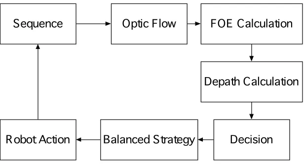
navigation. However, the main disadvantage of many of these is that they require two or more cameras (Kahlouche, 2007). However, robot obstacle avoidance systems can use optic flow with only one camera. Figure 2-2 shows the block diagram of such a navigation algorithm.

Sequence Optic Flow FOE Calculation

Depath Calculation

[image:18.595.151.459.244.412.2]

Balanced Strategy Decision Robot Action

Figure 2-2: The process flow of the obstacle avoidance system (Kahlouche, 2007)

Firstly, a sequence of images should be captured from the camera. Then, the system will perform the calculation of optic flow vectors from sequence images. In order to gain the orientation of the robot, the calculation of the focus of expansion (FOE) position in the image plane is necessary because the control law about “balanced

strategy” needs FOE information. The depth information is used to infer if the object is in the front of the robot or is close, or not, to the robot so that the robot can make a

(19)

2.5.1 Focus of expansion (FOE)

What is FOE? Actually, Kahlouche in his paper said (2007): “For translational motion

of the camera, image motion is directed away from a singular point corresponding to the projection of the translation vector on the image plane”. On the left side of the FOE point, the horizontal components of the optic flow of all points such as the

point(x,y) called h_L go towards to the left of the FOE point. And on the right side of the FOE point, the horizontal components of the optic flow of all points called

R

h points go towards to the right of the FOE point. The position of FOE is not always in the center of an image. Usually, the position is corresponding to a point where the divergence between the hL and hR is minimized. Similarly, the vertical location of the

FOE will minimize between the vertical components of optic flow called v_Randv_L. The question is how to estimate the position of the FOE in an image. Negahdaripour (1989) proposed a method to locate directly the focus of expansion. For our project, the robot should not have any operation about rotation. So the vertical location of the FOE point is not necessary to be calculated. The only thing that we need to care is about the horizontal location of the FOE point because it can be used to calculate the total numbers of the optic flow on both sides respectively in an image.

2.5.2 TTC (Time to Contact)

The time-to-contact (TTC) can be computed from the optical flow which is extracted from an image. Tresilian (1990) stated in his paper: “there is a method that can be used to calculate the TTC from the translation optical flow”. Basically, the image velocity can be divided into two parts depending on the rotational components Vr and the translational components Vt. As long as the global optic flow is computed is

(20)

2.5.3 The Balance Strategy

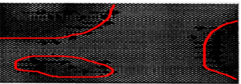
Kahlouche said: “when an object is close enough to the robot, it gives rise to faster

motion across the retina than farther objects. Also the object takes up more of the field of view, biasing the average towards their associated flow”. According to the value of optic flow, the robot turns away from the side of greater flow. There is a formulation that can be used to compute which side the optic flow is greater.

!

+ " = " # R L R L R L W W W W ) F F

( _r _r

v r

In here, "(F_L!F_R)is the difference between two sides of the robots’ body that can be

used to decide which side the robot should turn away from, and

_!

Wr_L is the sum

of the magnitudes of optic flow on the left side of an image.

_!

Wv_R is the sum of the magnitudes of optic flow on the right side of an image. Through the calculation based on this formulation, a robot can understand the difference between the left side and the right side in optic flow. If optic flow on the left side in an image is greater than the optic flow on the right side in an image, the robot can make a decision to turn right. Otherwise, the robot should turn left. The Picture 1 shows the balance strategy. It is clear to see the optic flow values and turning decision in the figure.

(21)

2.6 Camera

In the context of mobile robots, the quality of an image is captured by a camera with high quality. Basically, the quality level is determined by many things: illumination, lens and camera parameters (Camera parameters, 2007). One of the most important factors in camera parameters is offset. The offset is added to the CCD’s output signal

and increase all graylevels so that the image looks brighter. Actually, the camera parameter can be adjusted automatically by the camera itself. In Addition to what has

been motioned above, the lens is also important. The lens is an optical device which transmits and refracts light to form an image and should have perfect axial symmetry. Basically, a lens can consist of a single optical element. However, for a web camera, the quality of the offset and lens is very low.

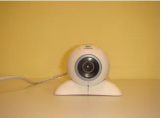
2.6.1 Logitech QuickCam

Logitech Quick camera (see in Figure 2-4) is a web camera, which can be used to connect to a personal computer by a USB cable. The eerie, eyeball-like camera comes with a base that fits on the top of a desktop. Usually, it has a resolution of 350,000 pixels, installs easily, and is used for the capture of E-mail photos and video as easily as text. The existing (packaged) software including drivers is quite useful as it can be used to calibrate images so that they can gain best effect. Usage proves that the image captured by this kind of camera is not perfect when compared to other expensive

(22)

[image:22.595.199.363.73.193.2]

Figure 2-4: The Logitech Quick Camera

2.7 OpenCV

What is OpenCV? Basically, OpenCV (Open source computer vision library 2007) is an open source library developed by Intel Corporation. The library can be installed

with some development tools such as visual studio, VB and so on to perform high level functions for computer vision and image processing because it is a collection of

C functions and C++ classes that include many vision algorithms (Jerome Landre 2003).

2.7.1 The Key Features

OpenCV is free for both non-commercial and commercial use. It provides a cross-platform middle-to-high level API that is about 300 C functions and a few C++ classes. Also OpenCV provides transparent interface to Intel Integrated Performance Primitives (User manual, 2007). Usually, OpenCV can be downloaded from the website: http://sourceforge.net/projects/opencvlibrary.

2.8 Visual C

(23)

easy to use Visual C to build up interfaces such as buttons, frames and other design elements.

2.8.1 C++

C++ is a popular language for the application development for Microsoft Windows. It is useful as a development language for vision applications as it can be combined with

OpenCV. It has functions to process some basic operations such as saving images, loading images and the conversion between the different image formats. Additionally,

(24)

Chapter 3

Methodology

This chapter indicates the methodology employed in testing the hypothesis in this project. It consists of four parts. The first part is about the measurement which is used to gather results and prove hypothesis. The second part is about assumptions which are used to narrow down the scope of the experiments in order to simply the whole project. The third part is some relative information about calibration and camera errors. Finally, there are experiment setup and experiment plans.

3.1 Measurement

In order to prove the hypothesis, measurement is necessary. There are three measurements: accuracy, time and simplicity

3.1.1 Accuracy

According to what have been mentioned in the literature review, the goal of robots is to avoid the obstacle in the view-field. So in here, the accuracy means if the robot can

make a right decision to prevent hitting an obstacle based on the optical flow coming from images captured by a web camera. In details, optical flow should be able to tell the robot which object is closer to itself so that it can make a decision for turning left or right.

3.1.2 Time

(25)

including taking image from a web camera and the computation of optic flow. This result is about the CPU process time and will be done within the program. Also the result about time will be compared to Thomas Grayston’s (2006) result in order to decide which method is best.

3.1.3 Simplicity

This qualitative estimate is used to identify which method requires the least equipments such as cameras, the personal computer and other equipment. Because the

low equipment cost is one of the goals of this study.

3.2 Assumption

According to the purpose of this study (time restriction and devices cost), the differential method for the computation of optic flow is used in all experiments. Although it requires very low equipment cost and low process time when it is compared to other methods such as correlation based methods, the error-rate is quite high because it is sensitive to noisy data. Also, the computation of optic flow based on this method is affected easily by the light condition, which means the light condition is quite important because it will affect the computation of the optic flow finally. In

addition, the web camera, does not like other professional cameras, has the high quality such as stability. So it is necessary to give few assumptions in order to

simplify these experiments and reduce the error rate.

3.2.1 Light Conditions

(26)

field of view of the camera is the same for all images. During testing, it was operated under the daylight lamp in the office.

3.2.1 Background Environment

The experiment environment should be quite clear. Doing this is to reduce the noisy data in every image so that the accuracy of the computation of optic flow based on the

differential methods is improved. In here, the assumption is that 1) only one obstacle in the field-view of the camera. 2) The background is clear, which means there should

be a wall with the stable color. 3) The surface of the obstacle is not crude.

3.2.2 FOE

FOE is the focus of expansion that can be used to compute the optic flow values. Usually, it is not always in the center of an image. However, in my experiments, it is necessary to assume the focus of expansion (FOE) in the center of an image in order to simply all experiments and make the computation for optic flow more straightforward. In this assumption, the robot should run on the flat ground. No matter which decision the robot turns, the location of the FOE will not change.

3.3 Making Decision

According to the method used in the prototype system of Kahlouche (2007), the robot should turn left when the total value of optic flow on the left side is less than the total value of optic flow on the right side in an image. Otherwise, it should turn right as the final decision. Through the computation of optic flow based on the differential

(27)

level, and the other is the value of optic flow in the vertical level. However, as information that has been mentioned above in the literature review, the robot does not do the rotation operation, so the value of optic flow in the vertical level can be ignored. So the decision for the robot turning is only based on the total value of optic

flow in the horizontal plane. The following text will show the computation method that is used for making decision.

For example, the size of the image is 2 x 6. Through a computation, the value of optic flow in the horizontal level in each pixel finally is stored into an array.

-100,90,-40,20,50,20 100,4,4,60,-33,-20

The method used to calculate the values of optic flow on the two sizes is: 1) Divide

the image into two parts which means the array will be divided into two components. So the total number of the values of optic flow on the left size is the sum of the values of all optic flow (in here:-100+90+(-40)+100+4+4+60 =+118). At the same time, the total number of the values of optic flow on the right size is 55(20+50+20+6-33-20 ) =+43. In here positive and negative symbol mean the direction of the optic flow. According to these two numbers: 118 and 43, the robot should turn right because the total number of the values of optic flow on the left size is greater than it on the right size.

3.4 Process Time Calculation

Process time mainly consists of two parts: the time for capturing one image from the web camera including reading frame from the video sequence and saving the image

(28)

GetTickCount() will be applied to calculate the time of CPU for any particular running program. When the program runs, the function will read the CPU time in the number of milliseconds. After the program finishes the particular process such as capturing images or making decision, the function will read the time of CPU again.

This calculation is based on the formula: process time = current time (the second reading) – past time (the first reading). Then the process time will be changed from milliseconds to seconds as the final result by using a formula: seconds = milliseconds/1000.

3.5 Calibration Image

The web camera does not have a high quality but it does implement an automatic exposure feature. The gain of the camera, and, hence the average brightness of the image is adjusted automatically so it is necessary to use another technology called calibration to improve the quality of the image as well. The technology is used to normalize an image captured from a web camera.

In details, it is better to use a white calibration card that is made of white paper with a fixed size about 3cm by 3cm. Usually, it is replaced on the left corner of the field-

view of the camera and near close from the camera itself, and appear at the same brightness level in every image. Firstly, the program used to calculate optic flow scans a region of 32 by 32 pixels on the left corner of an image captured by a web camera to sum the total number of the brightness values in this region. Secondly, divide the result by the size of region (in here, it is the total pixels of the while card: 32 x 32 =1024). Thirdly, it is necessary to assume the maximal brightness value in the color channel is 255.0, and then divide 255.0 by the result from the step two. Finally, multiply every pixel in the whole image by the result from the step three. The goal of

(29)

[image:29.595.215.370.124.240.2]

example, the Figure 3-1 with the explanation shows the whole procedure.

Figure 3-1: The calibration image

In the Figure 3-1, the white card is on the left corner of the field-view of the camera. The total number of the brightness values of the region with 32 x 32 is 220160 for example. Then divide 220160 by 1024=32 x 32, the result is 215 at average. Thirdly, divide 255 by 215 in order to get the brightness rate which can be used to normalize the whole image. Finally, multiply this with each brightness value in each pixel in the whole image.

3.6 Experiment Setup

This section presents the physical configuration of computer including program, camera and experimental environment used to conduct experiments

3.6.1 Computer Configuration

(30)

3.6.1.1 Visual Studio 6.0 and OpenCV

In some circumstances, the visual studio 6.0 is not directly installed into the computer by using “Step.exe” icon in the CD because of some reasons. So it is necessary to run a command in the “Run” windows in order to only install VC++ into the computer.

3.6.1.2 OpenCV Library

OpenCV should be installed into the computer with VC++ as well. It is possible to download the software called OpenCV1.0 from the website:

http://www.opencv.org.cn. The following pictures will show the procedure for the configuration of Opencv in Visual studio 6.0.

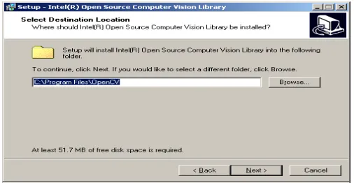
1) The default path for OpenCV is C:\program Files\OpenCV. It is easy to follow the interface to finish the install. However, it is necessary to add system variable into

C:\Program Files\OpenCV\bin. Figure 3-2, Figure 3-3 and Figure 3-4 show more details

(31)

Figure 3-3: The second step of the Install for OpenCV

Figure 3-0-4: The third step of the Install for OpenCV

[image:31.595.162.415.76.207.2]

2) After OpenCV is installed into the computer, the configuration of the library path must be done so that the program can run in this computer. Firstly, run the Visual studio C++ program, then select the “Option” option in the tool menu. Finally, set up the library path under Visual studio C++. The figure 3-5 shows the procedure.

Figure 3-5: The paths configuration for OpenCV library under the Visual Studio 6.0

(32)

[image:32.595.154.428.168.292.2]

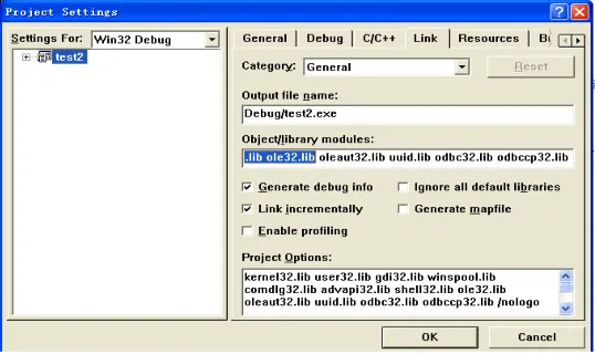
in five basic libraries: CXCORE, CV, High GUI, CVCAM and Machine Learning. Without these five libraries, it is impossible to compile the program. The following Figure 3-6 and Figure 3-7 show the procedure.

[image:32.595.163.432.367.527.2]

Figure 3-6: The first step of the paths configuration of OpenCV for a project

Figure 3-7: The second step of the paths configuration of OpenCV for a project

3.6.2 Camera

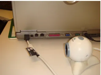
The web camera (Logitech) is connected to the personal computer by using a USB cable. The driver from CD also needs to be installed in the computer to support the

(33)

[image:33.595.198.362.72.194.2]

Figure 3-8: The camera is connected to the laptop by using a single cable

3.6.3 Experiment Environment

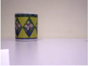
1) There is a piece of white paper with scale on the right side of the desktop. The purpose for doing this is to scale the distance between the obstacle and camera itself. In the center of the desktop, there is another piece of white paper that can be used to adjust the direction of the web camera so that the camera is projected towards to scene. (See in Figure 3-9)

Figure 3-9: The scale in the experiment environment

2) The background is the default wall with the grey color in the office. And the desktop is quite clear with white color. There are not other things except those

[image:33.595.211.375.411.533.2]

(34)

[image:34.595.212.374.73.195.2]

Figure 3-10: The background in the experiment environment

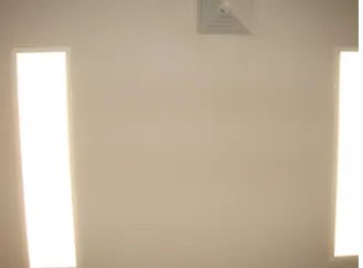
3) The light conditions in the experiment should be stable and good enough. There are

[image:34.595.217.381.316.437.2]

eight daylight lamps on the ceiling. During the whole experiment, these eight lamps should be on, and we assume that the light conditions are stable. (See in Figure 3-11)

Figure 3-11: The light condition in the experiment condition

[image:34.595.204.368.532.656.2]

4) The white card is made of A4 paper, which is used for calibration purpose.(See in Figure 3-12)

(35)

3.6.4 Experiment Plan

The experiments conducted are ultimately designed to test the hypothesis: if the

system can make a right decision to avoid an obstacle in the field-view of the camera. The standard for the right decision is the system will give the result about direction: turning left or turning right. However, it is not necessary to care about how much degree the robot should turn. In order to test this, it is first to conduct experiments examining the accuracy under the various conditions.

In this section, first, the error range of the web camera is examined. Secondly, the value of optic flow under the different light condition is examined. This is followed

by test that if the calibration image is necessary or not. Then there is another experiment that is used to test that if there is not any object in the field-view of the

camera based on optic flow. Then, there is a test that used to test the process time in order to measure if the method in this project is faster than another method used in Thomas’ project. Finally, there is a completed experiment that can be used to gain results and compared to Tahoma’s results to prove if the accuracy of this system is better than his.

3.6.4.1 Experiment Plan one:the error

range

The purpose of this experiment is to test the error range for the computation of optic flow. The main reason for that is the web camera is not designed for scientific research, so the precision degree about lens, offset and other camera parameters are not stable.

(36)

obstacle (here: cup) was placed on the left side of the field-view of the camera and 400cm far away from the camera. Firstly, the camera took a picture at the position: 0cm. Then a couple of minutes later, it took another picture. Finally, doing the computation of optic flow based on these two images is to show what the values of

optic flow looks like. The operation would be done for 10 times at the same position.

3.6.4.2 Experiment Plan two: the values of

optic flow under the different light

conditions

According to the information in the literature review, optic flow is sensitive for the light conditions. The purpose of this experiment is to test if the values of optic flow are easily affected by the light condition.

In this experiment, the camera was placed at the initial position: 0cm. And the

obstacle (here: cup) is also on the left side of the field-view and 400cm far away from the camera. The camera took a picture at 0cm, and moved to another position that was 380cm far away from the obstacle for taking another picture under the nominal light condition (Eight daylight lamps are open). The operation should be done each 20cm interval until 160cm far away from the initial position. Later, the procedure would be done again under another light condition (only Four daylight lamp is on).

3.6.4.3 Experiment Plan three: calibration

image test

(37)

accuracy in the computation of optic flow.

In this experiment, the camera was placed at the initial position: 0cm. And the obstacle (here: cup) is also on the left side of the field-view and 400cm far away from

the camera. The camera took a picture at 0cm, and took another picture in another position: 20cm without the calibration white card. This operation would be done each 20cm interval until the camera was on the position 160cm. Then repeat this operation with the calibration white card. All operations are under the normal light condition. (Eight daylight lamps are on)

3.6.4.4 Experiment Plan four: non-object

In the application of the robot navigation, it is necessary to adjust if there is an object in the field-view of the camera first. After that, the robot can make a decision to avoid the obstacle. So the purpose of this experiment is to test the values of optic flow to explain if there is no obstacle that exists in the front of the camera.

In this experiment, there is no object in the field-view of the camera. The camera took a picture in the initial position: 0cm, then took another picture at 20cm far away from the initial position, and then took the third picture at 40cm far away from the initial

position. The results about the values of optic flow were used to see if there is any implication between phenomenon and data.

3.6.4.5 Experiment Plan five: process time

In this experiment, the test is used to test how long the robot (program) should finish all procedures. In here, the procedures include two components: taking pictures and

(38)

Firstly, the camera was placed at the initial position: 0cm. The obstacle was on the left side and 400cm far away from the initial position. The camera took one picture per 10cm until 90cm far away from the initial position. The program returned the process

time for the each capture process. The average process time for the capture of pictures would be calculated. In addition, from these 9 pictures, the average process time for the computation of optic flow would be worked out as well.

3.6.4.6 Experiment plan six: last experiment

This experiment was to use the calibration images for the computation of the optic flow to test if the robot can make the right decision for turning (left or right).

(39)

Chapter 4

Results and Discussion

This chapter presents the results of experiments from 1-6 described in Chapter 3. And the meaning of these results is then discussed in the context of the hypothesis.

4.1 The implementation for OpenCV

and the meaning of values

The algorithm based on Horn’s principle about differential-based methods requires 6 parameters: the previous picture, the current picture, the horizontal component of the

optical flow of the same size as input images, the vertical component of the optical flow of the same size as input images, lagrangian multiplier and the criteria of termination of velocity computing. Once the program runs, it will computes the change of optic flow for every pixel, then the results about the horizontal components of optic flow and the vertical components of optic flow will be stored into two arrays, finally the program outputs the total number of optic flow for both sides and produce a turning decision. The following text will show the procedure with an example in order to explain where the numbers in the tables come from and what the numbers mean

There are two arrays used for the finial results: the vertical components of optic flow

and the horizontal components of optic flow -100,-20,30,40,90

-50,-60,43,80,20

(40)

From this array, we can see the value of optic flow in each pixel in the horizontal level has the direction and magnitude. After the horizontal components of the optic flow for all pixels have been calculated, the program will continue to calculate the total numbers of optic flow on both sides.

4.2 Results for the experiment one: the

error range

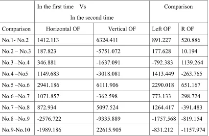
[image:40.595.86.513.339.616.2]

This Table 4-1 shows the results for the experiment one:

Table 4-1: The values of optic flow at the position: 0cm in the different time.

In the first time Vs

In the second time

Comparison

Comparison Horizontal OF Vertical OF Left OF R OF

No.1- No.2 1412.113 6324.411 891.227 520.886

No.2 – No.3 187.823 -5751.072 177.628 10.194

No.3 –No.4 346.881 -1637.091 -792.383 1139.264

No.4 –No5 1149.683 -3018.081 1413.449 -263.765

No.5 –No.6 2941.186 6111.906 2290.018 651.167

No.6 –No.7 1071.857 -362.598 773.133 298.724

No.7 –No.8 872.934 5097.524 1264.417 -391.483

No.8 –No.9 -2576.722 -9335.889 -1757.568 -819.154

No.9-No.10 -1989.186 22615.905 -831.212 -1157.974

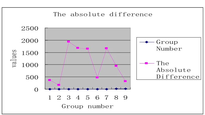
According to the theory, if the robot stays at the same position, the difference in the optic flow between two images taken by the camera in the different time but at the same position should be zero. However, the results show there is a difference between

(41)

[image:41.595.92.500.114.344.2] [image:41.595.230.366.632.744.2]

between these nine groups of data by using the formula: The absolute difference = |Left OF – Right OF|.

!"#$%&'()*+#$,-..#/#01#

2 322 4222 4322 5222 5322

4 5 6 7 3 8 9 : ; </(*=$0*>&#/

?%)*#'

</(*= @*>&#/

!"#

A&'()*+# B-..#/#01#

Figure 4-1: The absolute difference for the values of optic flow

Figure 4-1 shows the results for the absolute difference on values between the both sides respectively. It is clear to see that the range of the difference is from nearly 500 to almost 2000. This result can be used in the further experiments to determine which the value of the optic flow is true. For example, if the difference between the value of the optic flow on the left side and on the right side is in this range, which means the result would not be used to make a decision for a robot because it is probably caused by the error of the camera.

(42)

[image:42.595.233.363.134.243.2]

Figure 4-3: The camera was taken at another time

4.3 Results for the experiment two: the

values of optic flow under the different

light conditions

This experiment is used to test if the light conditions will affect the accuracy in robot

navigation.

The Table 4-2 and Table 4-3 show the result for the experiment two. In here, images were taken at the different position under two light conditions respectively: eight daylight lamps and four daylight lamps.

Table 4-2: Results for the light condition: eight daylight lamps

Eight daylight lamps

Comparison Horizontal OF OF on the left side OF on the right side Decision

0cm - 20cm 50071.379 81197.969 -31126.589 Right

20cm - 40cm 130322.043 81004.612 49317.431 Right

40cm - 60cm -2666.100 32255.665 -34921.766 Right

60cm – 80cm -22596.202 -18857.637 -3738.565 Left

[image:42.595.84.517.606.767.2]

(43)

100cm -120cm 68301.741 36210.016 32091.724 Right 120cm -140cm -55348.823 -40965.396 -14383.427 left 140cm– 160cm -67223.134 -21015.123 -46208.011 Right

In the table 4-2, there is one group data: No. 3 that would not be used to calculate the accuracy rate because the difference between values on the both sides was not out of the error range: 500-2000. So the valid data are only 8 groups. The accuracy rate was calculated by the formulary: the number of the right data/the total number of data.

[image:43.595.84.513.72.142.2]

Table 4-3: Results for the light condition: four daylight lamps

Four daylight lamps

Comparison Horizontal OF OF on the left side OF on the right side Decision

0cm -20cm 21471.761 14715.083 6756.677 Right

20cm-Vs 40cm 44037.894 51593.176 -7555.281 Right

40cm -60cm 17078.636 -5954.99 23033.632 Left

60cm-80cm 73786.797 12975.604 60811.192 Left

80cm-100cm 105772.406 110266.234 -4493.828 Right

100cm-120cm 14058.082 11522.753 2535.328 Right

120cm-140cm -42077.645 -33486.105 -8591.540 Left

140cm-160cm 34561.340 3768.985 30792.355 Left

(44)

!"#$%&&'(%&)$(%*#$+,$*"# -+..#(#,*$/+0"*$&1,-+*+1, 23 423 5223 6&&'(%&)$7%*# 8+0"*$&1,-*+1,9

6&&'(%&)

(%*#

:+0"* -%)/+0"* /%;<9 =1'( -%)/+0"* /%;<9

Figure 4-4: The accuracy rates for both light conditions

The figure 4-4 comes from the results in the table 4-3 and table 4-4. From the figure 4-4, it is clear to see the accuracy rate for making the right decision to avoid the obstacle under the light condition: eight daylight lamps, is 71%, which is better the accuracy rate under only four daylight lamps 50%. So the results tell us that the good light condition is important because it could enhance the accuracy rate of turning decision for robots

4.4 Results for the experiment three:

calibration image test

The purpose of this experiment is to test if calibration image can improve the accuracy rate.

[image:44.595.147.462.77.221.2]

The results are showed in Table 4-4 and Table 4-5

Table 4-4: Results for the computation of optic flow without calibration technique

Eight daylight lamps without the calibration technology Comparison Horizontal

OF

OF on the left side OF on the right side Decision

0cm- 20cm 11984.729 7198.074 4786.654 Right

(45)

40cm-60cm 52924.170 45605.438 7318.733 Right

60cm-80cm 455580.865 20367.724 25213.141 Left

80cm-100cm 41370.101 36550.113 4819.988 Right

100cm-120cm 58953.631 68635.815 -9682.183 Right

120cm-140cm 6123.987 -6879.016 13003.004 Left

[image:45.595.84.511.71.212.2]

140cm-160cm 23512.210 15623.174 7889.036 Right

Table 4-5: Results for the computation of optic flow with calibration technique

Eight daylight lamps with the calibration technology Comparison Horizontal

OF

OF on the left side OF on the right side Decision

0cm- 20cm 55778.425 30993.650 24784.775 Right

20cm-40cm 72208.688 45352.513 26856.175 Right

40cm-60cm 224800.735 194663.658 30137.077 Right

60cm-80cm -84953.787 -43515.809 -41437.977 Left

80cm-100cm 75174.112 48502.201 26671.911 Right

100cm-120cm 49371.676 46179.956 3191.719 Right

120cm-140cm 71937.250 88231.419 -16294.168 Right

140cm-160cm 63367.874 63911.284 -543.409 Right

[image:45.595.84.510.265.518.2]

(46)

!"#$%&'()*+,&-$./0/##-$0/&$%,*%1'+0)-%#+$,-$)%%1*)%2 *)0# 345 645 745 845 9%%1*)%2$:)0# !/&$%,*%1'+0)-%#+ 9%%1*)%2

*)0# ;')<#+$/,0"

%)=,.*)0,&-;')<#+$/,0"&10

%)=,.*)0,&-Figure 4-5: The accuracy rates for both circumstances: with calibration technique and without calibration technique

Figure 4-5 comes form the table 4-4 and table 4-5. It reflects the accuracy rate in the computation of optic flow with the calibration technology for robot turning is 88%, which is greater than it without calibration technology: 71%. The result tells us that actually the calibration images are quite useful for the computation of optic flow because it improves the accuracy rate.

4.5 The results for experiment four: no

object

[image:46.595.92.504.78.216.2]

In the robot navigation, it is important to infer if there is any obstacle in the front of the robot. In this experiment, the results show how the optic flow can be used to achieve the purpose. According to the experiment plan that mentioned in the methodology section, the original results are indicated in table 4-6.

Table 4-6: The values of the optic flow in two situations

No object in the front of the camera

Object in the front of the camera

[image:46.595.90.514.667.760.2]

(47)

40cm Vs 80cm -27349.972 -39046 299539.640 190837.920

80cmVs 120cm 6249.480 29971.61 -4659.50 33880.20

120cmVs160cm -3073.792 14135.076 282996.42 133583.784

!"#### !$#### !%####

#

%#### $####

#&'()*($#&'

$#&'()*(+#&'

+#&'()*(,%#&'

,%#&'()*(,"#&'

)-./0&12(34

56.0768/12(34

Figure 4-0-6: The values of optic flow in the vertical level and in the vertical level when there is no object in the front of the camera

!"####

#

"##### $##### %##### &#####

#'()*+)&#'(

&#'()*+),#'(

,#'()*+)"$#'(

"$#'()*+)"-#'(

[image:47.595.86.512.71.370.2]

*./01'23)45

67/1879023)45

Figure 4-7: The values of the optic flow in the vertical level and in the vertical level

[image:47.595.93.514.462.666.2]

(48)

The figure 4-6 and figure 4-7 shows the values of the optic flow in the horizontal level and the vertical level under the two different circumstances respectively. From these two figures, it is clear to see the total number of the values of the optic flow in the vertical level is quite small if there is not any object in the field-view of the camera.

Otherwise, it would be very large just like the values indicated in Figure 4-7. So if the implication is true, the values of optic flow in the vertical level can be used to infer if there is an obstacle in the front of the camera.

4.6 The results for the experiment five:

process time

In this experiment, time used to measure the capture of the images and making

[image:48.595.84.456.503.756.2]

decisions including the computation of the optic flow. The table 4-7 shows the original results.

Table 4-7: The times for the image capture and the computation of the optic flow in the different place

Distance (in cm)

Time for the image capture at each position (in seconds)

Making decisions (in seconds) 0 0.811

10 1.121

0.4

20 1.5. 30 0.912

0.51

40 0.72 50 0.912

0.34

60 1.3 70 1.82

0.52

(49)

90 0.62 !"#$%&'(%)*+,-("./%'.$%"#*/$ 01000 01200 31000 31200 41000

0)# 30)# 40)# 50)# 60)# 20)# 70)# 80)# 90)# :0)# ;'<","'.<

!"#$

[image:49.595.87.504.71.296.2]

!"#$%&'(%,=$%"#*/$%)*+,-($ *,%$*)=%+'<","'.

Figure 4-8: The time costs for the image capture The figure 4-8 shows the time for image capture in the ten different positions. Through the calculation, the average time for image capture is 1 second. In some positions, the requirement of time is over 1.5 seconds; the main reason was probably

due to the fan of CPU that was broken, so with the increase of temperature, the performance of CPU decreases. Besides, the other reason is probably due to some system processes suddenly running in the background.

!"#$%&'(%#)*"+,%-$."/"'+/ 0 012 013 014 015 016 017

0.#

_30.#

_50.#

_70.#

_80.#

9'/":"'+/

!"#$

;)*"+,-$."/"'+/

[image:49.595.94.490.501.720.2]

(50)

computation of optic flow. Through the calculation, it is easy to work out that the average time about making decisions is 0.418 second. At the position 20cm and position 40cm, the costs of time were greater than others. The main reason was probably as the same as above.

Actually, the whole procedure includes three components: the capture of two images, the computation of optic flow and making decision. So the total number for the whole procedure is 3.418 seconds (1.5s +1.5s +0.418). This means that the robot finishing one iteration to make a right decision will cost 3.418 seconds at least in my computer because this time does not include time about delay between taking the images. Of course, if the robot needs to deal with more computations, the cost of time for each iteration would be less. For example, if the robot needs to calculate the optic flow twice, it looks like four images are necessary. However, the image in the middle only needs to be captured once. So in this circumstance, the total number of time is 5.336s

at least (1.5s+1.5s+1.5s+0.418s+0.418s). In addition, the cost of time for the whole procedure is not fixed because the different computer with the different hardware will show the different time cost. The cost of the time showed above was based on the configuration of my computer: Inspiron 600m.

4.7 The results for the experiment six:

the final experiment

This experiment is used to test if the robot can make the right decision. The table 4-8 shows the original data coming from this experiment.

(51)

OF in the H and V level OF in the H level on the both sides

Distance Horizontal OF

Vertical OF OF on the left side

OF on the right side

Decision

0cm -20cm 151719.983 240884.276 89242.170 62477.812 Right 20cm-40cm 100117.296 145032.736 78150.274 21967.022 Right 40cm-60cm 26406.669 -27467.880 26939.97 -533.302 Right 60cm-80cm -33898.61 -385090.315 -15257.744 -18640.868 Right

!"#$%&'(#)$*+$,"#$*-,./$+'*0$.1$,"#$"*2.3*1,&'$'#%#'$&14$%#2,./&'$'#%#'

[image:51.595.84.514.89.452.2]

5677777 5877777 5977777 5:77777 5;77777 7 ;77777 :77777 977777 <*2.3*1,&'$=>$$ ?#2,./&'$=>$ =>$*1$,"#$'#+, ).4#$ =>$*1$,"#$2.@", ).4# !"#$%&'(#)$*+$,"#$*-,./ +'*0 A.),&1/#) B7/C5D7/C 87/C5B7/C :7/C587/C 7/C$5:7/C$

Figure 4-10: The values of optic flow on the both levels:

From this figure and table 4-8, we can see that when the robot was at the positions: 0cm and 20cm. The optic flow showed that robot should turn right. After the robot turned 20 degrees to the right, the change of the optic flow also showed that the robot

(52)

4.8 Results compared to Thomas’

As what have been discussed in the methodology section, there are three

measurements that are used to prove the hypothesis in this study.

4.8.1 Time Cost

In Thomas’s work, he used two cameras, two sensors and compass with the fuzzy

control system to perform the robot navigation. Two cameras were used to capture images in order to build up the depth information about the environment where the robot ran in first. After the cameras failed, the sensors and compass will take over as the input devices to input information to the system. In addition, it is impossible to capture two images at the same time in his work because the existing driver does not support two cameras operating at the same time. The only solution for him was to capture images by using two cameras in sequence. Actually in Thomas’ work, there is not any data about time that can be used to compare with my results. So it is difficult to give a conclusion about whose method requires less process time. However, it is possible to show the configuration lists of the personal computers between us (see in

[image:52.595.83.370.594.732.2]

Table 4-9 and Table 4-10).

Table 4-9: The details of the computer used in this study

The components Type

CPU Inter ® Pentium ® processor 1.50GHz Mother Board Intel 855GME

Memory 512MB

(53)

Table 4-10: The details of the computer used in Thomas’ project The components Type

CPU Mobile Intel ® Rentim® 4-m 1.8GHZ Mother Board Dell Latitude C840

Memory 512MB of RAM

Hard Disk IC25N020ATCS04-0 Video Card Geforce4 440

From these two tables, we can see the main difference between our computers is the frequency of the CPU used in Thomas’ work is higher than mine. That probably will

affect the cost of time for processing. In here, if we assume that: the cost of time for all processes in my project is as the same as that in Thomas’ project theoretically. The computer with the high CPU performance will save the time. That means the Thomas’s time cost might be less than mine.

Furthermore, according to the cost of the time for an iteration in this study mentioned in the section: 4.5 seconds, we can assume that the robot can travel in 117cm/s (400cm/3.148=117cm/s) speed in the assumed environment at best because we do not know if there is enough time for robot to make the turning action.

4.8.2 Simplify

The simplify means if the requirement of equipments in my project is less. For Thomas, he used two cameras, two sonar sensors, one digital compass and one laptop with the control system to conduct the robot navigation. However, in my project, the only equipments are the camera and the laptop. So in the aspect of simplify, my

(54)

4.8.3 Accuracy

From the results coming for experiment 6, the robot actually can make a right

decision for turning. After the application of the calibration technology, the accuracy for the computation of the optic flow has been improved dramatically. Compared to Thomas’ work, in this work, when the object is out of the view-field of the camera, the sensors and compass will take over and contribute to the system. However, in my work, from the results showed in the section 4.7, the robot can make the right decision for turning by still using the single camera; even the obstacle is out of the view-field of the camera. That means the camera could be used during the whole procedure without other devices. Of course, there are some disadvantages in my system. For

example, the optic flow does not show how far an obstacle is from the robot itself so that the robot does not determine if an obstacle is close enough to it, and must do the

(55)

Chapter 5

Conclusions

The purpose of this study was to test if using only one single web camera based on the bee vision algorithm combining the modified robot obstacle avoidance system is better than combining stereoscopic vision and sonar using a simplified fuzzy logic control system done by Thomas. The bee vision algorithm is to mimics the visual behavior of the bee to process captured images, which is based on the computation of the optic flow. Although the results have showed that the system can help robot make a right decision for turning, there are some problems that still exist. For example, it is difficult to measure the distance between the obstacle and the robot itself based on the optic flow. For robot, it is impossible to decide when it should turn. Furthermore, the method used for the computation of the optic flow is so sensitive for light conditions,

(56)

Chapter 6

Future work and development

This system based on optic flow has been designed to help robot perform navigation. However, there are still some aspects that need to be improved in the future.

6.1 FOE

FOE is used to maximize the divergence of optic flow, also is used to calculate the

total numbers of optic flow on the both sides in an image. However, the location of FOE is not always in the center of an image. Assuming the location of FOE in the center of an image will lead to the problem for the accuracy of the computation of the optic flow. So in the future, it is necessary to calculate the location of FOE in the real environment. The method used for locating the FOE was proposed by Shahriar Negahdaripour in 1987.

6.2 More information in the optic flow

Optic flow actually contains much information such as the distance between the bees and the obstacle. However, in this system, the application of optic flow did not show how far the robot is from the object. So it is difficult to measure the distance in order to decide if the robot does the turning action is timely. In the future, finding the

(57)

6.3 More objects in the view-field of the

camera.

In order to simplify this project, only one object in the front of the camera was

assumed. However, in the real-time environment, the robot needs to be able to avoid multi-obstacles in complicated environment. So how to use optic flow to distinguish

these obstacles in the view-field is a key question to success. In the future, if there is more time, the system will be expanded to deal with more than one obstacle and determine which obstacle is close enough to the robot itself, and must be avoided immediately.

6.4 Equipments

(58)

Reference:

1. Bin.L & Guang.S, 2003, Robotic Vision and Action Model based on a sort of optic flow computation, 24-5,

2. Camera parameters, 2007, The imaging Source Europe GmbH, viewed 28 October 2007,

<http://www.theimagingsource.com/en/resources/whitepapers/download/campara wp.en.pdf/>

3. Gibson J.J., 1950, The perception of the visual world. Boston, Houghton Mifflin. 4. Guilherme N. D &Avinash C. Kak, Vision for Mobile Robot Navigation: A Survey,

IEEE transactions on pattern analysis and machine intelligence, vol.24, No.2 February, viewed 18 October 2007,

< http://hyperphysics.phy-astr.gsu.edu/hbase/geoopt/foclen.html/>.

5. Horn B.K., 1981, Determining Optical Flow, Artificial Intelligence, p183-203.

6. Intel® Open Source Computer Vision Library 2007, User manual, Intel® Open Source Computer Vision Library, viewed 24 October 2007.

7. Jerome L., 2003, Programming with Intel IPP and Intel OpenCV: A beginner’s tutorial, Laboratore Electronique, p1.

8. Kahlouche S & Achour K., Optical Flow based robot obstacle avoidance, International Journal of Advanced Robotic System, Vol4, No.1, p13-16.

9. Liu G.F., 1997, The Technologies of Optical Flow, Journal of Southwest Jiaotong University, vol.20, No 10, December 1997.

10. Microsoft Developer Network, 2007, MSDN library, Microsoft Developer Network, viewed 13 September 2007,

<http://msdn2.microsoft.com/en-us/library/ms725473.aspx/>

11. Negahdaripour, S. & Horn, K.P., 1989, Direct method for locating the focus of expansion, Comp. Vis. Graph. Imp, Process. 46(3), 303-326, 1989.

(59)

<http://perception.inrialpes.fr/~Arnaud/vision/opencvman_old.pdf/>. 13. Owens, 2007, Energy-Based Methods, viewed 5 December 2007,

<http://users.fmrib.ox.ac.uk/~steve/review/review/node18.html/>.

14. Qian F., 2006, Optical Flow Computation Based on Correlation Coefficient, The

Journal of Electrical Integration, Vol 6.

15. Setiai Web, 2002, Honey Bee Navigation, viewed 5 October 2007, <http://www.setiai.com/archives/000064.html/>.

16. Shahriar N & Berthold K.P.H., 1987, A direct method for locating the focus of expansion, Massachusetts institute of technology artifical intelligence laboratory, A.I Memo No.939, January 1987.

17. Thomas.G., 2006, A simplified fuzzy-logic control system approach to obstacle avoidance combining stereoscopic vision and sonar, honors thesis.

18. Ulrich N & Suya Y., 1998, Integration of Region Tracking and Optical Flow for Image Motion Estimation, Computer Science Department Integrated Media