An analytical method for predicting 3D eddy current loss in permanent magnet machines based on generalized image theory

permanent magnet machines based on generalized image theory

.

White Rose Research Online URL for this paper:

http://eprints.whiterose.ac.uk/92577/

Version: Accepted Version

Article:

Chen, L., Wang, J. and Nair, S. An analytical method for predicting 3D eddy current loss in

permanent magnet machines based on generalized image theory. IEEE Transactions on

Magnetics. ISSN 0018-9464

https://doi.org/10.1109/TMAG.2015.2500878

(c) 2015 IEEE. Personal use of this material is permitted. Permission from IEEE must be

obtained for all other users, including reprinting/ republishing this material for advertising or

promotional purposes, creating new collective works for resale or redistribution to servers

or lists, or reuse of any copyrighted components of this work in other works.

[email protected] https://eprints.whiterose.ac.uk/ Reuse

Unless indicated otherwise, fulltext items are protected by copyright with all rights reserved. The copyright exception in section 29 of the Copyright, Designs and Patents Act 1988 allows the making of a single copy solely for the purpose of non-commercial research or private study within the limits of fair dealing. The publisher or other rights-holder may allow further reproduction and re-use of this version - refer to the White Rose Research Online record for this item. Where records identify the publisher as the copyright holder, users can verify any specific terms of use on the publisher’s website.

Takedown

If you consider content in White Rose Research Online to be in breach of UK law, please notify us by

An analytical method for predicting 3D eddy current loss in permanent

magnet machines based on generalized image theory

Liang Chen, Jiabin Wang, Senior Member, IEEE, and Sreeju. S. Nair, Student Member, IEEE

Department of Electronic and Electrical Engineering, The University of Sheffield, Sheffield, S1 3JD, United Kingdom

Abstract -- This paper proposes an analytical method, based on the generalized image theory, for accurate prediction of 3-dimensional (3D) eddy current distributions in the rotor magnets of permanent magnet machines and the resultant eddy current loss. The analytical framework is established in a 3D rectangular coordinate system, and the boundary conditions which govern the eddy current flows on the surfaces of magnets are represented by equivalent image sources in a homogenous 3D space extending into infinity. By introducing a current vector potential, the 3D eddy current distributions in magnets are derived analytically by employing the method of variable separation and the total eddy current loss in the magnets are subsequently established. The proposed method has been validated by 3D time-stepped transient finite element analysis (FEA). It is shown that the proposed method is extremely computationally efficient. When combined with 2D FEA of magnetic field distributions, the proposed method provides an accurate and computationally efficient means for predicting 3D eddy current loss in a variety of permanent magnet machines with due account of complex machine geometry, various winding configurations and magnetic saturation.

Index Terms— Eddy current, permanent magnet machines, image method

I. INTRODUCTION

Permanent magnet (PM) machines including surface mounted PM machines (SPM) and interior PM machines (IPM) are employed widely in industrial applications thanks to their high power density and high energy efficiency. The eddy current losses in the rotor magnets due to space and time harmonics of the armature reaction field may be significant. If this loss is not appropriately assessed and reduced, excessive rotor temperature may result which increases the risk of demagnetization, especially in high power or high speed PM machines. To reduce the eddy current losses, the magnets are usually segmented in circumferential and axial directions. This, however, increases magnet material waste and manufacturing cost.

In order to evaluate the eddy current losses in the magnets, various methods have been reported in a large number in literatures. In general, evaluation of rotor eddy current losses requires simultaneous solutions for the governing equations of the magnetic and eddy current fields. For radial field machines, it is reasonable to assume that the machine magnetic field is predominantly 2-dimesional (2D). As for the eddy current distribution, if the axial length of the magnets is much greater that their width and thickness, it may be sufficient to assume that the eddy current only flows in the axial direction. Thus, 2D numerical methods such as transient finite element analysis (FEA) can be used to calculate the eddy current losses [1]-[4]. To reduce the computation time, a number of 2D analytical methods have been developed for quantifying rotor eddy current losses in SPM with varying degrees of accuracy [5]-[10]. While 2D evaluation of eddy current loss in PM machines can be performed in a computationally efficient manner by either FEA or analytically, its accuracy is compromised if the axial length of magnets is comparable to their other dimensions since the eddy current flow in the magnets may become predominantly 3-dimensional (3D).

In order to evaluate eddy current loss in magnets more

accurately in PM machines which employ axial segmentations as a means of reducing eddy current loss, 3D FEAs are usually applied [11]-[16]. However, 3D FEAs are usually complicated, and their solutions require large memory and enormous computation time. In order to circumvent the problem, a multi-layer 2D FE based technique for quantifying the 3D eddy current field is proposed for axial flux PM machines [26]. However, this method is based on the assumptions that 1) the magnetic field in the normal direction in the air gap is uniform and 2) the boundary conditions on the two axial end planes of the magnets are negligible. These assumptions may incur large error when the air gap length is relatively large.

On the other hand, 3D analytical methods for calculation of eddy current loss have received significant interest in research communities to avoid the tremendous 3D FE computation [17]-[25]. However, because of complex geometry and high level of magnetic saturation in IPMs, the reported 3D analytical methods are only restricted to SPMs, and require one or more simplifying assumptions, such as:

1) Machine stator is slotless, and stator and rotor cores are infinitely permeable

2) Only radial flux densities exist in the magnets and air gap and they are independent of radial and angular positions;

3) Radial component of eddy current and the boundary conditions perpendicular to the radial direction are neglected;

These assumptions will inevitably compromise the accuracy of the eddy current loss predictions, particularly if the frequency of eddy current is relatively high, or its wavelength is relative short. Inaccurate eddy current loss calculation may cause underestimate of rotor temperatures, which in turn increases demagnetization risk. Therefore, an accurate and computationally-efficient solution for quantifying the eddy current losses is necessary.

to account boundary conditions of 3D eddy current flow. This method can be easily integrated with accurate analytical models for predicting magnetic field distribution to account slotting effect [27]-[30], or with 2D FEAs to quantify 3D eddy current loss in IPMs with complex geometry and under heavy magnetic saturations.

The rest of this paper is organized as follows. Section II describes the governing equations and boundary conditions for 3D eddy current field. Section III develops imaging techniques for accounting the boundary conditions of the eddy current field in rectangular magnets. Section IV presents analytical solutions for 3D eddy current distribution and expression for quantifying the eddy current loss in magnets. Section V illustrates the process of implementing the proposed 3D eddy current evaluation technique. Section VI validates the proposed technique on a SPM by comparison with 3D FEAs. Section VII summarizes the findings in conclusions. Appendix I provides a rigorous proof of the generalize image theory when applied to 3D current field problem. Appendix II lists the developed expressions for eddy current densities and eddy current losses.

II. FIELD DESCRIPTION FOR EDDY CURRENT IN RECTANGULAR MAGNETS

From Faraday’s induction law and neglecting eddy current reaction, the eddy current density distribution J in magnets at a given time instant is dependent on the rate of change of flux density B with time which can be seen as a source distribution denoted by S. Their relation is expressed as (1).

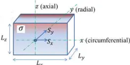
Fig. 1. A rectangular magnet in a permanent magnet machine with eddy current field excited by 2D magnetic field

× =

= , = , = (1)

where σ is the conductivity of magnets. According to the continuity law of the eddy current density, = 0, J may be expressed as the curl of a current vector potential A in (2).

× = (2)

And using the Coulomb gauge = 0, it can be shown that the current vector potential satisfies:

= (3)

Fig. 1 indicates a magnet in a PM machine in which the eddy current field is induced by 2D time-varying magnetic field. The magnet is approximated in rectangular shape by neglecting any curvature effect. The circumferential direction is denoted as x, radial direction as y and axial direction as z.

The flux density has x and y components which is independent of z. Thus, the source vector only has two components and . The dimensions of the magnets in the three directions are denoted as Lx, Ly and Lz, respectively.

Since the conductivity outside the magnet is zero, the boundary conditions on the 6 magnet surfaces, namely, two parallel x-z planes, two y-z planes and two x-y planes, are given by:

= 0 (4)

where nv denotes the normal vectors of the magnet surfaces.

However, analytical solution which satisfies (3) and (4) has not been established in literature because of the 3D nature and complexity of the problem.

For 2D static magnetic field problems with regular boundaries, image method has been widely used [31]-[33]. However, the applications of the image method in the eddy current field are rarely reported in literatures. The method described in [34] uses the concept of image to account for the 2D boundary conditions of a conducting plate in an eddy current damper. This leads to a reduction of the calculation error of eddy current loss compared with 2D prediction. However, the method did not address full 3D eddy current problems.

To date, the applications of the image method in 3D eddy current problems have not been found in literatures. This paper establishes the generalized image theory and the rules for 3D eddy current field solution, described in Appendix I. Based on these rules, the eddy current field in permanent magnets with 6 boundaries is analyzed below.

III. IMAGE METHOD SOLUTION FOR 3DEDDY CURRENT FIELD WITHIN A RECTANGULAR MAGNET

1) Image sources created for boundary conditions in two x-z planes

The eddy current field sources ( , , ) within the magnet boundaries (0 < , 0 < , 0 < ) maybe determined analytically or by 2D FEAs. According to the rule derived in Appendix I, to represent the effect of the right x-z boundary on the eddy current field, as shown in Fig. 2, the boundary is removed and an extra image source, denoted as

, is placed in the symmetrical position with respect to the boundary plane. The three vector components of the image have the same amplitude. The vector component whose direction is perpendicular to the boundary plane will have the same sign as that of the source, while the other two vector components change their signs. However, only two components need to be considered if the magnetic field is two-dimensional. The combined equivalent source ( , , )of the original and image sources after the first reflection on the right x-z plane is expressed in (5). is a vector constant used to represent the sign changes of the image vector components.

i and j are the unit vectors in the x and y directions,

respectively.

( , , ) = ( , , ), < , , , <

0 < , 0 <

= +

It should be noted that denotes component wise product of the two vectors, i.e., = + . Further, ( , , ) will be reflected by the left x-z plane as shown in Fig. 2 and have the second image, denoted as

and . The process of the reflections between the two parallel x-z planes continues, resulting in an infinite sequence of equivalent sources. Fig. 2 shows an arbitrary source S1 and

its images after three reflections. Table I lists the positions and signs of the original and image sources up to 5 reflections. It can be found that the original source S1 and its first image

source S2 form a pair expressed in (5), and all the images

repeat the pattern of the pair every 2Ly in ± y directions.

Therefore the resultant equivalent sources ( , , )

representing the combined effect of the source and the two x-z planes are expressed in the one dimensional periodic form given in (6).

( , , ) = , , ,

2 < 2( + 1) , = 0, ±1, ±2, … 0 < , 0 <

(6)

Fig. 2. Image sources created for boundary conditions on two x-z planes

TABLE I

CO-ORDINATES AND SIGNS OF THE ORIGINAL SOURCE AND IMAGES

Source and images y-coordinate Source signs

kx ky

… … … …

4 +1 +1

4 +1 -1

(second image on the left) 2 +1 +1 (second image on the left) 2 +1 -1 (original source) +1 +1 (first image on the right) = 2 +1 -1

+ 2 +1 +1

+ 2 +1 -1

+ 4 +1 +1

+ 4 +1 -1

… … … …

2) Image sources created for boundary conditions on the x-z and y-z planes

When the boundaries on the two y-z planes are also considered, as shown in Fig. 3, the sequence of images of the original source S1 derived for the two x-z planes will be further

reflected between the two parallel y-z planes. The consecutive reflections of the sequence form a 2D pattern which has periodicities of 2Lx and 2Ly in the x and y directions,

respectively. The repeated pattern is a set of the source and images denoted as S1, S2, S12 and S22 after the first reflection on

the right x-z plane and the subsequent first reflection on the top y-z plane. Their analytical expression is given in (7).

( , , )

=

( , , ), < , <

, , , < , <

( , , ), < , < ( , , ), < , <

0 < = +

(7)

The resultant equivalent sources ( , , ) representing the combined effect of the original source and the boundary conditions on the four planes are expressed in the two dimensional periodic form of (8).

( , , ) = , , ,

2 < 2( + 1) , 2 < 2( + 1) , 0 < , , = 0, ±1, ±2, …

(8)

Fig. 3. Image sources created for boundary conditions on two x-z planes and two y-z planes

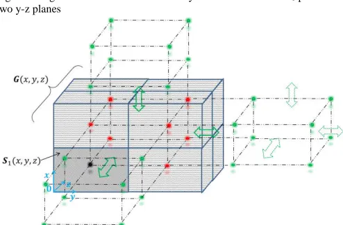
Fig. 4. Image sources created for boundary conditions on all the six planes

3) Image sources created for boundary conditions in y-z, x-z and x-y planes

images will be extended into infinite 3D volume, as seen in Fig. 4. The image distribution is periodic in all the x, y and z directions. The source and images to be repeated are formed from the first reflection with respect to the right x-z plane, followed by the first reflection with respect to the top y-z plane and the subsequent first reflection with respect to the front x-y plane. The group of the original source and 7 images, denoted by ( , , ), is defined in the region: 0 < 2 , 0 <

2 , 0 < 2 and given by (9):

( , , ) =

( , , ),

, , ,

, , ,

, , , , , ,

, , , ( , , ) ,

, , , =

(9) where

: 0 < , 0 < , 0 < : 0 < , < 2 , 0 < : < 2 , 0 < , 0 < : < 2 , < 2 , 0 < : 0 < , 0 < , < 2 : 0 < , < 2 , < 2 : < 2 , 0 < , < 2 : < 2 , < 2 , < 2

(10)

The final resultant equivalent source ( , , z, )

representing the combined effect of the original source and the boundary conditions on all the six planes are expressed in the three dimensional periodic form of (11):

( , , , ) = , ,

, ,

2 < 2( + 1) , 2 < 2( + 1) ,

2 < 2( + 1) , , , = 0, ±1, ±2, …

(11)

It follows that by employing the generalized image technique, the combined effect of the source ( , , ) and the boundary conditions can be represented by ( , , , )

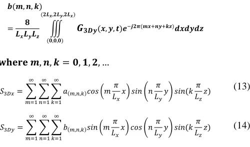
which is periodical in x, y, z directions. It may be further expressed as a 3D Fourier series given in (12)-(14).

( , , )

= ( , , ) ( )

( , , )

( , , )

(12)

( , , )

= ( , , ) ( )

( , , )

( , , )

, , = , , , …

= ( , , ) ( )

(13)

= ( , , ) ( ) (14)

a(m,n,k) and b(m,n,k) are the coefficients of the (m, n, k)th harmonic

for the x and y components of the equivalent sources respectively. They are easily calculated using fast Fourier transform (FFT) once the original source is known.

IV. EDDY CURRENT DISTRIBUTION AND TOTAL EDDY CURRENT LOSS

For each harmonic _{( , , )} and _{( , , )}, the source is

distributed sinusoidally within an infinite isotropic 3-dimensional space. Hence, the solution to (3) may be found by the method of variable separation for each harmonic of the order ( , , ). The resultant current vector potential is obtained in (15) and (16)

= ( , , ) ( ) (15)

= ( , , ) ( ) (16)

The eddy current density is derived from (2) as:

= ( , , ) ( ) (17)

= ( , , ) ( ) (18)

= ( , , ) ( ) (19)

Since each harmonic is orthogonal, the total eddy current loss at a given time instant is the sum of the losses associated with each harmonic component:

= ( , , )

= 1

8

1

[ ( , , ) + ( , , )

+ ( , , ) ]

= ( , , )+ ( , , )+ ( , , )+ ( , , )

+ ( , , )

(20)

current vector potential and eddy current densities, and p1(m,n,k)

- p5(m,n,k) for the total eddy current loss are all arithmetic

functions of the harmonic order and magnet dimensions. They are summarized in Appendix II.

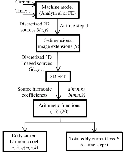
V. METHOD IMPLEMENTATION A. Computation process

The process of computing 3D eddy current loss in rotor magnets employing the analytical technique described in sections III and IV is illustrated in the flowchart of Fig. 5. The 2D magnetic field as the source function may be calculated analytically using the more accurate subdomain model [27] with due account of slotting effect. Alternatively, the magnetic field distribution may be obtained from 2D FE in which case complex geometry and heavy magnetic saturation often seen in IPMs can also be easily dealt with. If the 2D FEA includes eddy current effect, the reaction field of the eddy current is, to some extent, approximated in the 3D evaluation [11]. In addition, if the magnetic field solver can take eddy current distribution as its input, the resultant eddy current density from the image method may be fed back to the magnetic solver. The iterations repeat until convergence is achieved. However, this is not studied in this paper.

Due to the periodicity, the original and image sources are represented by 3D harmonic series in free space. In order to perform FFT of the combined sources, the magnetic field distribution obtained from analytical or FE prediction need to be discretized in the x, y, z dimensions. Therefore the accuracy of the sources and their resultant eddy current field depends on the harmonic numbers (m × n × k) that are considered in the calculations, which, in turn, determines the number of samples of the magnetic field in the x-y-z magnet region which are used in FFT. To account for the high order space harmonics caused by a winding configuration, slotting, magnetic saturation and step change of the image sources across the boundaries, the number of discretization samples should be sufficiently large. In order to speed up discrete FFT, the sample numbers are chosen as the integer power of 2. It is shown by comparing the eddy current losses with different numbers of samples that the loss converges to sufficient accuracy with 32 × 32 × 32 samples. When calculating the eddy current loss at the rated current and the max speed with 6 axial segments and none circumferential segments for the machine under study, the relative differences of the results with 32 × 32 × 32 samples and 64 × 64 × 64 samples, compared with the results with 128 × 128 × 128 samples, are 0.212% and 0.0429%, respectively.

The eddy current distribution is calculated at each time step. Because time varying eddy current densities usually repeat 6 or 12 times in a fundamental electric period, it is necessary to calculate the eddy current loss at least for one sixth or one twelfth of the electrical period to obtain the average value.

Since the calculations are performed in 3-dimensional space for each harmonic, matrix operations are used to facilitate efficient calculations of (9) - (20). When the magnetic field within the magnets are sampled with 64 × 64 × 64 points in

the x-y-z directions, which means the harmonic orders (m, n, k) are also accounted up to 64 × 64 × 64, the total calculation time, including the analytical prediction of the magnetic field and the eddy current loss calculations, is ~10 seconds on a typical 3.10 GHz, 32GB PC in Matlab environment. As a comparison, in order to perform 3D time-step FEs, apart from the geometry and physical model construction and meshing process, the computation time on the same PC is 82 hours for the case of non-axial-segmentation and 7.5 hours for the case of 18 axial segmentations.

B. Magnetic 3D end effect and magnet curvature effect

Because of the influence of the end windings and the fringe effect, the flux density due to the armature winding and magnets decreases in the regions close to the axial ends of the machine lamination stack. Numerous work have been undertaken to examine the phenomenon analytically [35][36] and by 3D FE [37][38]. It is shown in these studies that the affected length of the air gap in the axial direction is approximately equal to the radial thickness of the equivalent air gap which is the sum of the magnet thickness and air gap. The ‘affected region’ is defined as the region in which the flux density drops below 99% of the value that exists in the middle of the axial length. At the end of the axial length, the flux density is 70% ~ 80% of the value in the middle, depending on the equivalent air gap thickness. Thus, in most radial field machines in which the axial length is sufficiently large than the equivalent air gap, the 3D end effect is negligible. For the machine under study in the paper, the length of magnets affected by the 3D end effect is ~5% of the total stack length, and the 3D effect on the eddy current loss should be negligible. However for the other machine designs with short stack lengths compared to the equivalent air gap, the 3D end effect on the magnetic field and the eddy current loss may

Fig. 5. Flowchart of 3D eddy current calculation using generalized image method

Machine model (Analytical or FE)

3-dimensional image extensions (9) Current

Time: t

Discretized 2D

sources S(x,y) At time step: t

Discretized 3D imaged sources

G(x,y,z)

3D FFT

Source harmonic coefficiencts

a(m,n,k), b(m,n,k)

Arithmetic functions (15)-(20)

Eddy current harmonic coef.

e, h, q(m,n,k)

need to be carefully assessed before application of the proposed technique. If the 3D end effect is significant, 3D magneto-static field solutions may be obtained and used together with the proposed technique to compute the eddy current loss, albeit the computation time will be much longer.

As for circular-shaped magnets, a conventional process which approximates the arc shapes to rectangular shapes should be applied. It should be noted that the curvature effect becomes prominent when the magnets have a large angle and large radial thickness. However, this is less likely in a practical machine for ease of magnet assembly and for reduction of eddy current loss.

VI. VALIDATIONS BY 3DFEAS

The proposed method for analytical predicting 3D eddy current loss in PM machines has been validated by 3D FEAs.

A. Machine topology and design parameters

The proposed method is applied to a 5kW 18-slot 8-pole SPM machine as shown in Fig. 6, for evaluation of the eddy current loss in the rotor permanent magnets. The machine employs winding design features [39] to reduce space harmonics and hence rotor eddy current loss, while retaining the merits of fractional slot per pole machine topology. The key geometrical and physical parameters and specifications are listed in Table II.

Fig. 6. Cross-sectional schematic of 18-slot 8-pole SPM machine

TABLE II MACHINE PARAMETERS

Items Value

Rotor radius 32.5 mm

Magnet outer radius 37.5 mm Stator inner radius 38.45 mm

Stack length 118 mm

Magnet resistivity 1.8 × 10

Rated Ampere turns per coil 513.5

Max. speed 4500 r/mim

Rated current 80 A

Rated torque 35 Nm

B. 2D FE for field source validations

2D magnetic field distributions of the machine are obtained analytically as described in [5] and the resultant time derivations of flux density distributions form the source for the eddy current calculation. For simplicity, magnetic saturation and effect of slotting are neglected. This will not lead to large error when the machine runs at the Maximum Torque per Ampere (MTPA) mode [4].

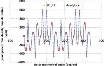
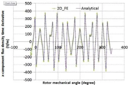
Fig. 7 to Fig. 10 compare the analytically and 2D FE predicted variations of the magnetic flux density components and their time derivatives with angular position at a given time instant of ωt = 15o (elec.) when the machine operates at the maximum speed of 4500 r/min and rated current, where ω is the fundamental electric angular frequency of the operation. It can be seen that the analytical predictions agrees very well with those obtained from the 2D FEAs. This ensures the accuracy of the source of excitation of the eddy current distribution to be analytically predicted by the proposed method. The dominant time varying harmonics of the source for eddy current field can be assessed from these results, but because of the length limit, they are not included in this paper.

Fig. 7. y-component variation of flux density with angular position

along the mean radius of magnets at ωt = 15o (elec.)

Fig. 8. y-component variation of flux density time-derivative with

angular position along the mean radius of magnets at ωt = 15o (elec.)

Fig. 9. x-component variation of flux density with angular position

Fig. 10. x-component variation of flux density time-derivative with

angular position along the mean radius of magnets at ωt = 15o _(elec.)

C. Comparisons of eddy current distribution and eddy current loss with 3D FEAs

A 3D FE model of the machine, as shown in Fig. 11, has been built to predict the 3D eddy current distribution and resultant eddy current loss induced in the magnets. Since the machine employs fractional slot per pole topology, circumferential symmetry exists only over 180 mechanical degrees. Thus, a quarter of the machine has to be modelled in 3D FEAs. Tangential magnetic field boundary condition is imposed on the two end surfaces perpendicular to the axial direction. Consequently, the magnetic field will be confined in the 2D x-y plane. This implies that the end (3D) effect of magnetic field distribution is neglected. In addition, perfect insulation boundaries are applied to the end surfaces of the magnets. The time-stepped 3D FEs considers the BH curves of the real iron laminations. The field in the conducting parts of magnets is governed by:

× ( × / ) = ( / + ) (21)

= ( / + ) (22)

in which Am, and are the magnetic vector potential,

permeability and electric scalar potential, respectively. The model is meshed to make sure the predicted eddy current loss being sufficiently accurate. The total number of the nodes for the model without axial segmentation is approximately 2×106.

Fig. 12 compares analytically and 3D FE predicted z-component eddy current density distributions at ωt = 15o (elec.) on the surface (defined by y = 0.5Ly, 0 < x < Lx, 0.5Lz <

z < Lz) of the second magnet piece on the right in Fig. 11 when

the machine operates at the maximum speed and rated current. Each magnet per pole is segmented into 2 pieces circumferentially and 14 pieces axially. Fig. 13 compares analytically and 3D FE predicted variations of z-component eddy current density with circumferential position (x) at ωt = 15o (elec.) y = 0.5Ly and z = 0.75Lz. Good agreement between

the two can be observed albeit the effect of mesh discretization is clearly visible in the 3D FE predictions.

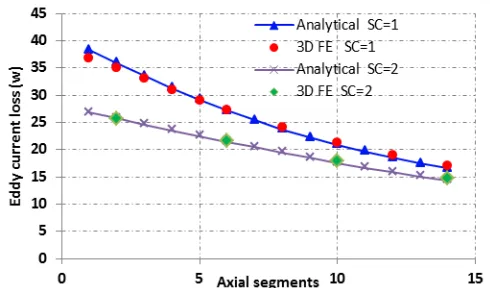
Fig. 14 compares analytically and 3D FE predicted total eddy current loss variations with time when the machine operates at the maximum speed and rated current with each magnet per pole segmented by 2 circumferentially. Fig. 15

compares analytically and 3D FE predicted eddy current loss variations with number of axial and circumferential segments per pole. It can be seen that in all cases, good agreements are obtained between the 3D FE and analytical results. Owing to neglect of the magnet curvature effect, the analytical results deviate slightly from the FE predictions when the magnets in each pole are not circumferentially segmented (SC=1).

Fig. 11. 3D FE machine model

(a)

(b)

Fig. 12. Z-component eddy current density contours on the surface defined by (y = 0.5Ly, 0 < x < Lx and 0.5Lz < z < Lz) at ωt = 15o (elec.): (a): Analytical;

Fig. 13. Variations of analytically and 3D FE predicted z-component eddy current density with circumferential position x at ωt = 15o _{(elec.), y = 0.5L}

y

and z = 0.75Lz.

Fig. 14. Comparison of 3D FE and analytically predicted total eddy current loss variations with time when machine operates at the maximum speed and rated current with each magnet per pole segmented by 2 circumferentially

Fig. 15. Analytically and 3D FE predicted eddy current loss variations with the number of axial and circumferential segments. The number of circumferential segments is denoted by SC

VII. CONCLUSIONS

A computationally efficient and accurate means for predicting 3D eddy current loss in rotor magnets of PM machines has been developed based on the generalized image theory. The developed method has been validated by 3D FEAs on an 18-slot, 8-pole SPM machine. It has been shown that the developed method only takes about 10 seconds for computing 3D eddy current loss in contrast to more than 24 hours of computation time required by 3D FEA, representing computational efficiency improvement by 5 orders of magnitude.

Although the effectiveness of the developed method is only demonstrated on a SPM machine in the paper due to length limit, the method can be used to evaluate 3D eddy current loss

in a variety of PM machines which have complex geometry and exhibit high level of magnetic saturation when it is combined with 2D FE analysis of the magnetic field distributions. The utility of the method for assessing 3D eddy current loss in IPM machines will be reported in future publications. The method is also applicable to PM machines in which the magnets are placed on the stator, such as flux-switching PM machines, etc.

Since the method is derived for the magnets with rectangular shapes, for PM machines with circular shaped magnets, the predictions may incur small errors in PM machines with low number of pole-pairs and when circumferential segmentation is not employed. However, these conditions are in minority. Nevertheless, modifications of the method in a cylindrical co-ordinate system need to be further studied.

The developed method provides a very efficient and effective tool for assessing the influence of axial and circumferential segmentations of magnets on eddy current loss as a part of design optimization process.

APPENDIX I:DERIVATION OF THE GENERALIZED IMAGE METHOD FOR 3DEDDY CURRENT FIELD

A. Images for 3D eddy current field in two infinite conducting regions

Without loss of generality, consider two infinitely large conducting regions as shown in Fig. 16 (a). Region 1 has conductivity and occupies the space where > 0 and the rest is denoted as region 2 with conductivity . A source of excitation, ( , , ), is located in region 1.

(a)

(b) (c)

Fig. 16. (a) Two semi-infinite conductors with sources in region 1; (b) equivalent image sources in region 2 for eddy current field in region 1; (c) equivalent image sources in region 1 for eddy current field in region 2.

To quantify the field distribution in region 1, the effect of the boundary conditions may be represented by the image,

{ ( , , ), ( , , ), ( , , )}, in region 1 with the conductivity in region 2 being set to , as shown in Fig. 16 (c). , , and , , are image

coefficients to be determined to satisfy the boundary conditions given in appendix I-B.

Since the field region in Fig. 16 (b) is now homogenous and extends to infinite, the current vector potential A which satisfies = in region 1 can be obtained from the volume integration:

=

4 + 4 d d d

= ( ) + ( ) + ( )

= ( ) + ( ) + ( + )

(23)

=

4 + 4 d d d (24)

= (

4 + 4 )d d d (25)

The current vectors in region 2 are similarly derived as:

=

4 + 4 d d d

(26)

=

4 + 4 d d d (27)

= (

4 + 4 )d d d (28)

B. Image coefficients satisfying boundary conditions

The interface conditions at the boundary between regions 1 and 2 that eddy current density J and electric field strength E must satisfy are given by:

= (29)

= (30)

= ₍₃₁₎

which can be further expressed in terms of the current vector potentials as

= (32)

1

= 1 (33)

1

= 1 ₍₃₄₎

Applying the current vector potentials given in (23)-(28) to (32)-(34), the image coefficients are determined and given in (35) and (36).

= = = =

+ (35)

= =

+ (36)

When region 2 is non-conductive, = 0, then

= = 1, = 1 (37)

In summary, to represent the effect of an infinite boundary at z = 0 on the eddy current field, the boundary may be removed and an extra image source is placed in the symmetrical position with respect to the boundary plane in non-conducting region 2. The three components of the image vector have the same amplitude. The z component has the same sign as the source, while the x and y components whose directions are in parallel with the boundary plane have the opposite signs to the source.

APPENDIX II:SOLUTIONS TO THE EDDY CURRENT FUNCTIONS The coefficients, c(m,n,k), d(m,n,k), e(m,n,k), h(m,n,k), q(m,n,k) for the

current vector potential and eddy current densities, and p1(m,n,k)

- p5(m,n,k) for the eddy current loss are defined as follows:

Let = ( ) + ( ) + ( ) (38)

( , , )=

( , , )

(39)

( , , )=

( , , ) ₍₄₀₎

( , , )=

( , , )( ) ₍₄₁₎

( , , )=

( , , )( ) ₍₄₂₎

( , , )=

( , , ) ( , , )( )

(43)

( , , )= ( , , ) ₈ (44)

( , , )= ( , , ) ₈ (45)

( , , )= ( , , ) ₈ (46)

( , , )= ( , , ) ₈ (47)

( , , )= 2 ( , , ) ( , , )

1

8 (48)

REFERENCES

[1] K. Yoshida, Y. Hita, K. Kesamaru, "Eddy-current loss analysis in PM of surface-mounted-PM SM for electric vehicles," IEEE Trans. Magnetics, vol.36, no.4, pp. 1941-1944, Jul. 2000

[2] N. Zhao, Z. Q. Zhu, W. Liu, "Rotor eddy current loss calculation and thermal analysis of permanent magnet motor and generator," IEEE

Trans. Magnetics, vol.47, no.10, pp.4199-4202, Oct. 2011

[3] H. V. Xuan, D. Lahaye, M. J. Hoeijmakers, H. Polinder, J. A. Ferreira, "Studying rotor eddy current loss of PM machines using nonlinear FEM including rotor motion," in Proc. XIX International Conference on

Electrical Machines (ICEM), 2010, pp.1-7, Sept. 2010

[4] L. Chen, J. Wang, " Evaluation of rotor eddy current loss in permanent magnet machines employing fractional-slot windings with low space harmonics", in Proc. IEEE International Magnetics Conference,

Intermag Europe 2014, Dresden, Germany, May 4-8, 2014

[5] J. Wang; K. Atallah; R. Chin, W. M. Arshad, H. Lendenmann, "Rotor Eddy-Current Loss in Permanent-Magnet Brushless AC Machines,"

[6] A. Rahideh, T. Korakianitis, "Analytical magnetic field distribution of slotless brushless permanent magnet motors – Part 1. Armature reaction field, inductance and rotor eddy current loss calculations,", IET Electric

Power Applications, vol.6, no.9, pp.628-638, November 2012

[7] K. Yamazaki, Y. Fukushima, "Effect of Eddy-Current Loss Reduction by Magnet Segmentation in Synchronous Motors With Concentrated Windings," IEEE Trans. Industry Application, vol.47, no.2, pp.779-788, March-April 2011

[8] P. Sergeant, Van Den Bossche, "Segmentation of Magnets to Reduce Losses in Permanent-Magnet Synchronous Machines," IEEE Trans.

Magnetics, vol.44, no.11, pp.4409-4412, Nov. 2008

[9] F. Dubas, A. Rahideh, "Two-Dimensional Analytical Permanent-Magnet Eddy-Current Loss Calculations in Slotless PMSM Equipped With Surface-Inset Magnets," IEEE Trans. Magnetics, vol.50, no.3, pp.54-73, March 2014

[10] Y. Amara, P. Reghem, G. Barakat, "Analytical Prediction of Eddy-Current Loss in Armature Windings of Permanent Magnet Brushless AC Machines," IEEE Trans. Magnetics, vol.46, no.8, pp.3481-3484, Aug. 2010

[11] K. Yamazaki, Y. Kanou, "Rotor Loss Analysis of Interior Permanent Magnet Motors Using Combination of 2-D and 3-D Finite Element Method," IEEE Trans. Magnetics, vol.45, no.3, pp.1772-1775, March 2009

[12] T. Okitsu, D. Matsuhashi, Yanhui Gao; K. Muramatsu, "Coupled 2-D and 3-D Eddy Current Analyses for Evaluating Eddy Current Loss of a Permanent Magnet in Surface PM Motors," IEEE Trans. Magnetics, vol.48, no.11, pp.3100-3103, Nov. 2012

[13] J. D. Ede, K. Atallah, G. W. Jewell, J. B. Wang, D. Howe, "Effect of Axial Segmentation of Permanent Magnets on Rotor Loss in Modular Permanent-Magnet Brushless Machines," IEEE Trans. Industry

Application, vol.43, no.5, pp.1207-1213, Sept.-oct. 2007

[14] Y. Aoyama, K. Miyata, K. Ohashi, "Simulations and experiments on eddy current in Nd-Fe-B magnet," IEEE Trans. Magnetics, vol.41, no.10, pp.3790-3792, Oct. 2005

[15] K. Yamazaki, A. Abe, "Loss Investigation of Interior Permanent-Magnet Motors Considering Carrier Harmonics and Magnet Eddy Currents,"

IEEE Trans. Industry Application, vol.45, no.2, pp.659-665,

March-April 2009

[16] K. Yamazaki, M. Shina, Y. Kanou, M. Miwa, J. Hagiwara, "Effect of Eddy Current Loss Reduction by Segmentation of Magnets in Synchronous Motors: Difference Between Interior and Surface Types,"

IEEE Trans. Magnetics, vol.45, no.10, pp.4756-4759, Oct. 2009

[17] S. Ruoho, T. Santa-Nokki, J. Kolehmainen, A. Arkkio, "Modeling Magnet Length In 2-D Finite-Element Analysis of Electric Machines,"

IEEE Trans. Magnetics, vol.45, no.8, pp.3114-3120, Aug. 2009

[18] W.-Y. Huang; A. Bettayeb, R. Kaczmarek, J. C. Vannier, "Optimization of Magnet Segmentation for Reduction of Eddy-Current Losses in Permanent Magnet Synchronous Machine," IEEE Trans. Energy

Conversion, vol.25, no.2, pp.381-387, June 2010

[19] M. Mirzaei, A. Binder, C. Deak, "3D analysis of circumferential and axial segmentation effect on magnet eddy current losses in permanent magnet synchronous machines with concentrated windings," in Proc.

XIX International Conference on Electrical Machines (ICEM), 2010,

Sept. 2010

[20] M. Mirzaei, A. Binder, B. Funieru, M. Susic, "Analytical Calculations of Induced Eddy Currents Losses in the Magnets of Surface Mounted PM Machines With Consideration of Circumferential and Axial Segmentation Effects," IEEE Trans. Magnetics, vol.48, no.12, pp.4831-4841, Dec. 2012

[21] J. Pyrhonen, H. Jussila, Y. Alexandrova, P. Rafajdus, J. Nerg, "Harmonic Loss Calculation in Rotor Surface Permanent Magnets— New Analytic Approach," IEEE Trans. Magnetics, vol.48, no.8, pp.2358-2366, Aug. 2012

[22] B. Aslan, E. Semail, J. Legranger, "Analytical model of magnet eddy-current volume losses in multi-phase PM machines with concentrated winding," in Proc. Energy Conversion Congress and Exposition

(ECCE), 2012 IEEE , pp.3371-3378, Sept. 2012

[23] Sang-Yub Lee; Hyun-Kyo Jung, "Eddy current loss analysis in the rotor of permanent magnet traction motor with high power density," in Proc.

Vehicle Power and Propulsion Conference (VPPC), 2012 IEEE ,

pp.210-214, Oct. 2012

[24] Peng Zhang; G. Y. Sizov, Jiangbiao He; D. M. Ionel, N. A. O. Demerdash, "Calculation of magnet losses in concentrated-winding permanent magnet synchronous machines using a Computationally Efficient - Finite Element method," in Proc. Energy Conversion

Congress and Exposition (ECCE), 2012 IEEE , pp.3363-3370, Sept.

2012

[25] B. Aslan, E. Semail, J. Legranger, "General Analytical Model of Magnet Average Eddy-Current Volume Losses for Comparison of Multiphase PM Machines With Concentrated Winding," IEEE Trans. Energy

Conversion, vol.29, no.1, pp.72-83, March 2014

[26] H. Vansompel, P. Sergeant, L. Dupre, "A Multilayer 2-D–2-D Coupled Model for Eddy Current Calculation in the Rotor of an Axial-Flux PM Machine," IEEE Trans. Energy Conversion, vol.27, no.3, pp.784-791, Sept. 2012

[27] L. J. Wu, Z. Q. Zhu, D. Staton, M. Popescu, D. Hawkins, "Analytical prediction of electromagnetic performance of surface-mounted PM machines based on subdomain model accounting for tooth-tips," IET

Electric Power Applications, vol.5, no.7, pp.597-609, August 2011

[28] T. Lubin, S. Mezani, A. Rezzoug, "2-D Exact Analytical Model for Surface-Mounted Permanent-Magnet Motors With Semi-Closed Slots,"

IEEE Trans. Magnetics, vol.47, no.2, pp.479-492, Feb. 2011

[29] B. Hannon, P. Sergeant, L. Dupré, "2-D Analytical Subdomain Model of a Slotted PMSM With Shielding Cylinder," IEEE Trans. Magnetics, vol.50, no.7, pp.1-10, July 2014

[30] B. N. Cassimere, S. D. Sudhoff, D. H. Sudhoff, "Analytical Design Model for Surface-Mounted Permanent-Magnet Synchronous Machines," IEEE Trans. Energy Conversion, vol.24, no.2, pp.347-357, June 2009

[31] P. Hammond, "Electric and magnetic images," in Proc. the IEE - Part

C: Monographs , vol.107, no.12, pp.306-313, September 1960

[32] C. J. Carpenter, "The application of the method of images to machine end-winding fields," in Proc. the IEE - Part A: Power Engineering, vol.107, no.35, pp.487-500, October 1960

[33] B. Hague, The Principles of Electromagnetism Applied to Electrical

Machines, Dover, 1962

[34] K. J. W. Pluk, T. A. van Beek, J. W. Jansen, and E. A. Lomonova, " Modeling and Measurements on a Finite Rectangular Conducting Plate in an Eddy Current Damper," IEEE Trans. Ind. Electron., vol. 61, no. 8, pp. 4061–4072, August 2014

[35] H. Bolton, "Transverse Edge Effect in Sheet-rotor Induction Motors," in

Proceedings of the Institution of Electrical Engineers, vol.116, no.5,

pp.725-731, May 1969

[36] T. W. Preston, A. B. J. Reece, "Transverse Edge Effects in Linear Induction Motors," in Proceedings of the Institution of Electrical

Engineers, vol.116, no.6, pp.973-979, June 1969

[37] Ranran Lin, A. Arkkio, "Calculation and Analysis of Stator End-Winding Leakage Inductance of an Induction Machine," IEEE Trans.

Magnetics, vol.45, no.4, pp.2009-2014, April 2009

[38] Dong Li, Weili Li, Xiaochen Zhang, Jin Fang, Hongbo Qiu, Jiafeng Shen, Likun Wang, "A New Approach to Evaluate Influence of Transverse Edge Effect of a Single-Sided HTS Linear Induction Motor Used for Linear Metro," IEEE Trans. Magnetics, vol.51, no.3, pp.1-4, March 2015

[39] J. Wang, V. I. Patel, W. Wang, "Fractional-Slot Permanent Magnet Brushless Machines with Low Space Harmonic Contents," IEEE Trans.