Forensic Face Sketch Recognition

IJEDR1904007 International Journal of Engineering Development and Research (www.ijedr.org) 29

Forensic Face Sketch Recognition

1Divya T M 1Guest faculty

1University Visvesvaraya College of Engineering

_____________________________________________________________________________________________________

Abstract - A forensic sketch is matched with a database of images. A professional forensic sketch artist draws a sketch of a suspect’s face by listening to a description given by witness. A database has a collection of sketches and images. A much efficient recognition system is implemented in this paper in order to recognize a forensic sketch. firstly, the feature vectors of the face are extracted from both the sketches and images using SIFT & MLBP descriptors. Later the nearest neighbor matching is implemented to match the feature vectors of sketches and images. secondly, the same feature vectors obtained from SIFT & MLBP are further revised to reduce the dimension of SIFT & MLBP feature vectors. A linear Discriminant Analysis is implemented. In this approach, A multiple projection of slices of feature vectors are made. The images in the database are first converted into pseudo-sketches, then the matching of pseudo-sketches with the forensic sketch is done by minimum distance recognition. The two standard databases are CUHK & IIIT-D of sketches and images are used. The recognition rates for both the approaches are compared.

keywords - Forensic sketch, Recognition, CUHK database, IIIT-D database, SIFT, MLBP, LFDA.

_____________________________________________________________________________________________________

I. INTRODUCTION

A wide range of techniques and algorithms have been proposed and implemented for Face recognition under different pose, lighting and expression of faces. However, there has been relatively less attraction towards sketch recognition. This Sketch Recognition plays a very important role in the law enforcement. However, in many cases of crimes like murder, Robbery, Accident, Sexual assault, the only witness is the victim. A professional sketch artist draws a sketch by the verbal description stated by the victim. These sketches are called as forensic sketch. Once the sketch is completed, an automated Recognition system that would match the drawn sketch with the images in the database maintained by law enforcement officials.

In this paper, a combined technique to match a forensic sketch with the database is proposed. The normal face recognition system needs modification because the sketches and images are two different entities. This Recognition system poses a great challenge because A witness may not exactly remember the criminal’s appearance. These sketches are often incomplete and inaccurate. The remaining sections of this paper are organized as follows. Section II states a related work of the algorithm. Section III explains SIFT & MLBP feature descriptor based Nearest Neighbor Matching. Section IV explains LFDA based Minimum Distance Matching. Section V gives Result analysis using Matlab simulation. Finally, section VI conclusion of this paper.

Figure 1: Viewed Sketch and its photograph Figure 2: Forensic sketch and its photograph II.RELATED WORK

The Forensic Face Sketch Recognition System requires a database of forensic sketches and these are not much easily available. Most of the face sketch recognition system is implemented for the viewed sketches, sketched that are drawn by looking at the person not just by the verbal description. A small number of sketches were used in the database. Major research work in matching these viewed sketches was done by Tang et al. [3], [2], [5], [6], [7]. In his approach, a digital image obtained from a sketch and face is matched using recognition algorithm. In SIFT based approach, the feature vectors are extracted from sketches and images, and used for matching though the face and sketches modalities are different, the feature vectors extracted from an image and sketch contains the information necessary for recognition. [13].

In this paper, A similar feature based SIFT is used to match the sketches with image. In addition to SIFT, A Multi-scale local binary pattern, histogram based feature description is also used. A similar matching algorithm is used by Liao. [14].

And finally both these large feature vectors are arranged into many slices of smaller dimension using an efficient discriminant classifiers, LFDA proposed by Lei & Li.[15].

III. SIFT AND MLBP BASED SKETCH RECOGNITION

IJEDR1904007 International Journal of Engineering Development and Research (www.ijedr.org) 30 uniformly distributed sub-regions of the face, these vectors are sampled. The sampling points are selected by two entities, a patch size ‘p’ and a displacement size ‘d’. The patch size ‘p’ is the size of the square window over which the feature vector of an image is computed. The displacement size ‘d’ is the patch displacement for each sample in terms of number of pixels. The difference (p-d) gives the overlapping pixels of two adjacent patches.

The sampling points are computed. A PXP size window slides across the image. An image is of size HXW. The horizontal sampling locations(M) given by M=(H-P)/(d+1) and similarly vertical locations points (N), N=(W-P)/(d+1), next an image feature vector ‘ɸ’ is computed of size ‘t’. These feature vectors are concatenated into one dimensional feature vector ɸ of size (MXNXt). Later a Nearest Neighbor sketch matching is implemented on the feature vectors.

A. Scale Invariant Feature Transform feature Descriptor Algorithm

SIFT is a Scale-invariant feature transform [11]. SIFT is a feature descriptor algorithm which is used to extract the necessary feature vectors from an image. This was published by David Lowe. The important points of an image are the feature description vectors. These vectors should be detectable even if there is any different in scaling, noise and background interference and lighting of an image, such invariant vectors extracted from test sketch are compared with the feature vectors of an image in the database. The vectors which are invariant under any conditions extracted will lie in high contrast regions like in the edges of an image. SIFT is one such feature vector extraction algorithm and the vectors extracted are invariant under any circumstances and reduces errors caused due to variations.

The steps involved in the extraction are Step 1: Building a Blurred image:

The original image is I (x, y) where x, y are coordinates of an image I. A several octaves of the original image is generated. Every octave generated is half the size of the previous octave. In an octave, images are blurred using the Gaussian blur.

B (x, y, σ) represents the blurred image. G (x, y, σ) represents blur operator. Where σ is the amount of blur parameter. Mathematically, the blurred image is obtained by convoluting Gaussian blur G (x, y, σ) and original image I (x, y).

B (x, y, σ) = G (x, y, σ) * I (x, y) (1) where σ being the blur operator, higher the value, higher the blur.

Step 2: Detecting keypoint locations

The two consecutive images in an octave are subtracted and repeat this process for all the octaves. These images are the

approximated scale invariant of Gaussian. These are useful for detecting keypoints. The difference of Gaussian images is D(x, y, σ).

D(x, y, σ)= B(x, y, kσ)- B(x, y, σ). (2) where B(x, y, kσ) is scaled k times the B(x, y, σ).

Step 3: Locate Maxima and minima points

Each point of D (x, y, σ) is compared neighbor points up with its eight neighbor point which lie in the same scale and nine neighbor points up and down which lie in different scale as shown in figure 4. The Extrema point is the minimum or maximum value of these point, these are the keypoints generated.

IJEDR1904007 International Journal of Engineering Development and Research (www.ijedr.org) 31 Step 4: Elimination of Low Contrast and Edgy Regions

In this step firstly, the keypoints which have low contrast and keypoints along edges are eliminated. The keypoints are further refined using Taylor expansion. The magnitude of the intensity of the current pixel of a difference of Gaussian image is less than the defined value, that keypoint is eliminated. Secondly, two gradients are calculated for a keypoint which is perpendicular to each other. The keypoints obtained can be flat, in these flat region, the two gradients will be small. Along an edge, one gradient will be large and another gradient will be small and the last region is corners, in this both gradients are large. The corner region gradients are retained, other edges and flat gradients are rejected. This can be mathematically obtained by hessian matrix.

Step 5: Assigning Orientation to keypoints using histogram.

Histogram is an estimation of probability distribution of gradients of keypoints. It identifies the most prominent gradient. A group of gradients are assigned to one keypoint if there is only one peak. Suppose there are many peaks above 80 to 85% mark, these are all converted to new keypoint. A distinct feature vector of 128 numbers is generated from this.

B. Generation of Multiscale Local Binary Pattern Feature vectors

An image is partitioned into sub-windows. In each window Multiscale Local Binary pattern histograms are obtained, normalized and concatenated into one feature vector of that window. A 16 X 16 window of pixels is taken, this is further split into 16, 4 X 4 subwindows, A histogram of 8 equal parts called bins are generated. The gradient orientation from the above 4 X 4 sub -window is placed into appropriate 8 bins, this is repeated for 16, 4 X 4 sub--windows. The value 128 number of feature vectors are normalized. Finally, these features obtained have sufficient information to determine an image identity. This features are well suited for Sketch Recognition.

Figure 5: Sampling Scheme Figure 6: Histogram levels of MLBP

C. System Architecture of SIFT and MLBP

A sketch or corresponding photos are pre-processed. An image is split into patches. Each patch with a size of P X P. The SIFT feature vectors are computed for each patch of an image. An image of size W X H, hence many such features has to be computed for a single image because image has high resolution. A window of size P X P slides across the image in raster scan technique. An M X N SIFT features are computed as discussed in section III. Finally, a set of V-128 dimensional features for each image V= M-N.

Figure7: System Architecture of SIFT & MLBP features

(a)Training set of sketch/photo correspondence; (b) pre-processed image; (c)SIFT & MLBP features

D. Nearest Neighbor Matching Approach

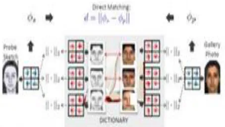
For Nearest Neighbor Matching, The difference between a sketch and an image is given by D. 𝑫 = ||∅𝒔 − ∅𝒑||𝟐 (3)

IJEDR1904007 International Journal of Engineering Development and Research (www.ijedr.org) 32

Figure 8: Nearest Neighbor Matching Approach

IV. Linear Feature Discriminant Analysis

Each image is divided into 16 X 16 patch, this produces 128 SIFT feature vectors, these feature vectors are further refined using LFDA technique. In this Linear Feature Discriminant Analysis, each feature vectors are arranged into slices. These slices are of smaller dimension. These smaller dimension slices are concatenation of feature vectors of each column of a patch. A LFDA is applied on each slice. This involves Principal Component Analysis to remove redundant information in the slices and a final feature vector is extracted.

A. System Architecture of LFDA

There are M X N array of patches consisting of SIFT vectors. A slice for each of N columns of the patch is created. For a feature vector of d-dimension, a (M*d) dimensional N slices are created. A training set has a sketch and images of n persons. This results in 2n training set. The feature vector of sketch is represented as ∅𝑠𝑖 = 𝐹(𝐼𝑠𝑖) and similarly image is ∅𝑝𝑖 = 𝐹(𝐼𝑝𝑖), these feature vectors are combined as column vector. This is represented as 𝑋𝑠= [∅1𝑠, ∅2𝑠… … ∅𝑠𝑛] for the sketch and 𝑋𝑝=

[∅1𝑝, ∅𝑝2… … ∅𝑝𝑛] for images. The combined column vector is 𝑋 = [∅1𝑠, ∅𝑠2… … ∅𝑠𝑛 ∅𝑝1, ∅𝑝2… … ∅𝑝𝑛] finally PCA whitening is performed on these combined vectors.

(a) (b) (c) (d) Figure 9: System Architecture of LFDA features showing

(a)Training set of sketch/photo correspondence; (b) pre- processed image;(c)SIFT & MLBP features; (d)LFDA features B. Face Sketch Synthesis System

The images in the database are first synthesized into sketches using photo Eigen space synthesis system then matching is performed in the same modality that is sketch Eigen space using Minimum distance. This section deals with photo to sketch transformation. The sketch differs from an image in texture and shape. The texture and shape are separated. The Eigen transformation is done separately for the shape and the texture as shown in figure 10. The shape of the face is represented as a graph. A graph contains a set of fiducial points shown in figure11. The shape of the sketch and an image are linear. The fiducial

points of sketch and image will be in same position. The texture transformation is based on grayscale around the fiducial points.

Figure 10: Framework of the Face Sketch Synthesis System. Figure 11: Fiducial graph model.

The steps involved in the synthesis of sketch are as follows:

IJEDR1904007 International Journal of Engineering Development and Research (www.ijedr.org) 33 2) Apply transformation of shape and texture for a sketch 𝑮𝒔.

𝑮𝒔= 𝑬(𝑮𝒑− 𝑮𝒑𝒎) + 𝑮𝒑 (4)

(a) (b) (c) Figure 12: Face Sketch Synthesis Results

Face photo (b) synthesized sketches using separate Eigen transformation on texture and shape (c) real sketch

C. Minimum Distance Matching

The Eigen vectors of the images and the input sketch are computed and compared.

Figure 13: Minimum Distance Matching Step 1: Compute the image Eigenspace 𝐄𝐩= 𝐀𝐩𝐕𝐩𝐀𝐩

−𝟏_𝟐

using image training set, where 𝐀𝐩= [𝐩𝟏 − 𝐦𝐩, … . , 𝐩𝐌 − 𝐦𝐩] =

[𝐏𝟏′′_{, … , 𝐏𝐌]}

is the image sample matrix. Similarly compute the sketch Eigen space 𝑬𝒔 using 𝑨𝒔 for the sketch. Step 2 : Use 𝑬𝒑 to compute the pseudo sketch 𝑺𝒓′ where 𝑺𝒓 = ∑𝑴𝒊=𝟏𝒄𝒊𝑺𝒊 + 𝒎𝒔 for each image in the database.

Step 3 : Compute Eigen weight vector 𝑾𝒑′ = 𝑬𝒔𝑻𝑺𝒓′ for 𝑺𝒓′ in 𝑬𝒔. Similarly for Eigen weight vector 𝑾𝒔′ = 𝑬𝒔𝑻𝑺𝒌′ for 𝑺𝒌′ (probe sketch ) in 𝑬𝒔.Finally the one with the minimum distance between 𝑾𝒔′ and 𝑾𝒑′ is classified as sketch with its corresponding face.

V. RESULTS and DISCUSSIONS

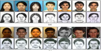
The two databases were used: CUHK database shown in Figure 14(a) and IIIT-D sketch database shown in Figure 14(b) Database

The CUHK sketch dataset has sketches and image pairs. They have same background and constant illumination. The IIIT-D dataset has also sketches and image pairs.

Figure 14: Sketch-digital image pairs from the (a) CUHK database and (b) IIIT-D database Result Analysis

IJEDR1904007 International Journal of Engineering Development and Research (www.ijedr.org) 34 Table 1.1: Recognition Rates for the proposed methods

Database Training/Testing Images Algorithm Accuracy

CUHK 78/233 SIFT & MLBP 97.33%

LFDA 99.47%

IIT-D

58/173 SIFT & MLBP 75.24%

LFDA 76.24%

VI. CONCLUSION

Recognition of face image photographs from the sketches is a challenging task. The sketches are inaccurate and incomplete. Matching these sketches with digital face offers many difficulties because of grey level changes and even the shape of the sketch and image. The key contribution of the above proposed combined algorithm is making use of SIFT and MLBP feature vectors of sketches and images. This offered a good performance rates. Later A Discriminant Analysis is applied on these SIFT and MLBP vectors to reduce the dimensionality. The performance was further improved by LFDA. A large database need to be collected to understand and analyze the complexity in Forensic sketch recognition.

REFERENCES

[1] B. Klare and A. Jain, “Sketch to Photo Matching: A Feature-Based Approach,” Proc. SPIE Conf. Biometric Technology for Human Identification VII, 2010.

[2] X. Tang and X. Wang, “Face Sketch Recognition,” IEEE Trans. Circuits and Systems for Video Technology, vol. 14, no. 1, pp. 50-57, Jan. 2004.

[3] Q. Liu, X. Tang, H. Jin, H. Lu, and S. Ma, “A Nonlinear Approach for Face Sketch Synthesis and Recognition,” Proc. IEEE Conf. Computer Vision and Pattern Recognition, pp. 1005-1010, 2005.

[4] J. Zhong, X. Gao, and C. Tian, “Face Sketch Synthesis Using E-HMM and Selective Ensemble,” Proc. IEEE Conf. Acoustics, Speech, and Signal Processing,2007.

[5] X. Wang and X. Tang, “Face Photo-Sketch Synthesis and Recognition,”IEEE Trans. Pattern Analysis and Machine Intelligence, vol. 31, no. 11,pp. 1955-1967, Nov. 2009.

[6] X. Tang and X. Wang, “Face Sketch Synthesis and Recognition,” Proc. IEEE Int’l Conf. Computer Vision, pp. 687-694, 2003.

[7] D. Lin and X. Tang, “Inter-Modality Face Recognition,” Proc. European Conf.Computer Vision, 2006.

[8] X. Gao, J. Zhong, J. Li, and C. Tian, “Face Sketch Synthesis Algorithm Based on E-HMM and Selective Ensemble,” IEEE Trans. Circuits and Systems for Video Technology, vol. 18, no. 4, pp. 487-496, Apr. 2008.

[9] B. Xiao, X. Gao, D. Tao, and X. Li, “A New Approach for Face Recognition by Sketches in Photos,” Signal Processing, vol. 89, no. 8, pp. 1576-1588, 2009.

[10] W. Liu, X. Tang, and J. Liu, “Bayesian Tensor Inference for Sketch-Based facial Photo Hallucination,” Proc. 20th Int’l

Joint Conf. Artificial Intelligence,2007.

[11] Y. Li, M. Savvides, and V. Bhagavatula, “Illumination Tolerant Face Recognition Using a Novel Face from Sketch

Synthesis Approach and Advanced Correlation Filters,” Proc. IEEE Int’l Conf. Acoustics, Speech and Signal Processing, 2006.

[12] H. Nizami, J. Adkins-Hill, Y. Zhang, J. Sullins, C. McCullough, S. Canavan,and L. Yin, “A Biometric Database with

Rotating Head Videos and Hand-Drawn Face Sketches,” Proc. IEEE Conf. Biometrics: Theory, Applications, and Systems, 2009.

[13] D. Lowe, “Distinctive Image Features from Scale- Invariant Keypoints,” Int’l J. Computer Vision, vol. 60, no. 2, pp.

91-110, 2004.

[14] S. Liao, D. Yi, Z. Lei, R. Qin, and S. Li, “Heterogeneous Face Recognition from Local Structures of Normalized Appearance,”

Proc. Third Int’l Conf. Biometrics, 2009.

[15] Z. Lei and S. Li, “Coupled Spectral Regression for Matching Heterogeneous Faces,” Proc. IEEE Conf. Computer Vision

and Pattern Recognition, pp. 1123- 1128, June 2009.

[16] B. Klare and A. Jain, “Heterogeneous Face Recognition: Matching NIR to Visible Light Images,” Proc. Int’l Conf. Pattern

Recognition, 2010.

[17] T. Ojala, M. Pietika¨inen, and T. Ma¨enpa¨a¨, “Multiresolution Gray-Scale and Rotation Invariant Texture Classification

with Local Binary Patterns,” IEEE Trans. Pattern Analysis and Machine Intelligence, vol. 24, no. 7, pp. 971-987,July 2002.

[18] K. Mikolajczyk and C. Schmid, “A Performance Evaluation of Local Descriptors,” IEEE Trans. Pattern Analysis and

Machine Intelligence, vol. 27, no. 10, pp. 1615-1630, Oct. 2005.

[19] T. Ahonen, A. Hadid, and M. Pietikainen, “Face Description with Local Binary Patterns: Application to Face

Recognition,” IEEE Trans. Pattern Analysis and Machine Intelligence, vol. 28, no. 12, pp. 2037-2041, Dec. 2006.

[20] B. Klare, Z. Li, and A. Jain, “On Matching Forensic Sketches to Mug Shot Photos,” MSU Technical Report