Pattern formation in large domains

This is a repository copy of

Pattern formation in large domains

.

White Rose Research Online URL for this paper:

http://eprints.whiterose.ac.uk/176/

Article:

Rucklidge, A.M. (2003) Pattern formation in large domains. Philosophical Transactions Of

The Royal Society Of London Series A - Mathematical Physical and Engineering Sciences,

361 (1813). pp. 2649-2664. ISSN 1471-2962

https://doi.org/10.1098/rsta.2003.1267

[email protected] https://eprints.whiterose.ac.uk/ Reuse

See Attached

Takedown

If you consider content in White Rose Research Online to be in breach of UK law, please notify us by

Pattern formation in large domains

B y A. M. R u c k l i d g e

Department of Applied Mathematics, University of Leeds, Leeds LS2 9JT, UK

Published online 3 November 2003

Pattern formation is a phenomenon that arises in a wide variety of physical, chemical and biological situations. A great deal of theoretical progress has been made in understanding the universal aspects of pattern formation in terms of amplitudes of the modes that make up the pattern. Much of the theory has sound mathematical justi¯cation, but experiments and numerical simulations over the last decade have revealed complex two-dimensional patterns that do not have a satisfactory theoretical explanation. This paper focuses on quasi-patterns, where the appearance of small divisors causes the standard theoretical method to fail, and ends with a discussion of other outstanding problems in the theory of two-dimensional pattern formation in large domains.

Keywords: pattern formation; quasi-patterns; small divisors

1. Introduction

There is a diverse collection of physical, chemical and biological systems that natu-rally organize themselves into patterns. In these various situations, the same types of qualitative behaviour appear repeatedly, and universal mathematical models have been developed to understand each characteristic situation. These mathematical models of pattern formation provide a unifying viewpoint and have, in turn, stim-ulated further research in the relevant experimental disciplines. Pattern formation remains a topic of great current interest that spans diverse areas of pure mathematics, applied mathematics and experimental science.

One well-studied example of a pattern-forming instability is the Faraday wave problem of the formation of waves on the surface of a layer of °uid as it is driven by vertical vibrations. This system has been subjected to intensive scrutiny in lab-oratory experiments and has come to be regarded as an archetypal pattern-forming system. Clear examples of pattern formation occur in a wide range of other systems, including Rayleigh{B¶enard convection, liquid crystals in externally imposed electric ¯elds, nonlinear optics, directional solidi¯cation, vibrated granular media, chemical reactions, and catalytic oxidation.

Laboratory experiments in pattern formation have continually prompted theoret-ical developments, and the phystheoret-ical insights that they reveal are essential to a com-plete understanding of these phenomena. Numerical simulations have also played a central role, and with advances in experimental technique and computing power,

One contribution of 22 to a Triennial Issue `Mathematics, physics and engineering’.

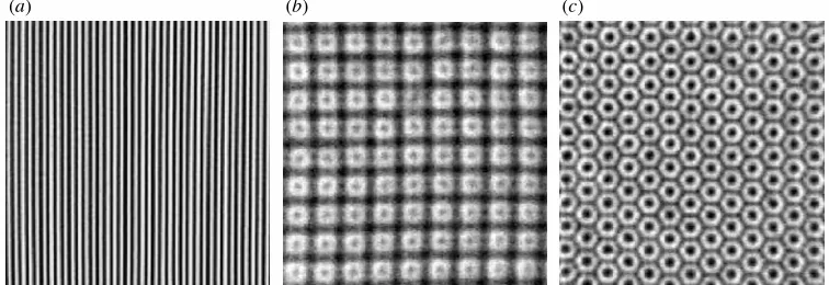
(a) (b) (c)

Figure 1. Examples of experimentally observed patterns, viewed from above. (a) Stripes (straight rolls) in Rayleigh{B¶enard convection. (Reproduced with permission from Cakmuret al. (1997). Copyright (1997) American Physical Society.). (b), (c) Squares and hexagons in a two-frequency forced Faraday wave experiment. (Reproduced with permission from Arbell & Fineberg (2002). Copyright (2002) American Physical Society.) Note the extraordinary degree to which the pat-terns display spatial periodicity, as well as rotation and re°ection symmetry.

attention has turned from smaller to larger domains. Many new types of behaviour have been discovered in recent years, including quasi-patterns and spiral defect chaos. Theoretical understanding of these new types of behaviour is very much lacking, in some cases, apparently, for deep mathematical reasons.

The simplest patterns|stripes, squares and hexagons|have re°ection, rotation and translation symmetries; experimentally observed examples of these are shown in ¯gure 1. A comprehensive and very successful theory has been developed to analyse the creation of these patterns from an initial featureless state. This theory, which is based on computing the amplitudes of the various waves (or modes) that make up the pattern, is known as equivariant bifurcation theory, and is expounded in detail in a series of texts (see, for example, Golubitsky & Stewart 2002).

In order to apply rigorous mathematical theories to explain experimental results and other occurrences of pattern formation in the natural world, there are naturally a series of idealizations and approximations that must be made. The ¯rst assumption concerns modelling: the experimental con¯guration is supposed to be describable in terms of some set of equations that predict the future evolution of the system, given its current state. The evolution laws often take the form of partial di®erential equations (PDEs), particularly when the system under consideration involves a °uid. In many situations, the next idealization is to suppose that in the absence of any driving force, the system will remain featureless, and that if the forcing is turned up, it must reach a critical level before it can overcome any inherent dissipation in the system. If the level of forcing (which is a parameter under the control of the experimentalist) exceeds this critical value, the featureless state will be unstable, and any small disturbances will grow. These cannot grow for ever, and one possible outcome is that the system will settle down to a steady state with some degree of spatial structure: a pattern.

con-(a) (b) (c)

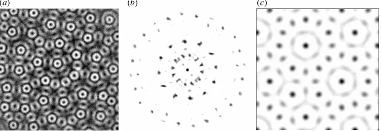
Figure 2. Quasi-patterns: (a) 12-fold quasi-pattern observed in a two-frequency forced Faraday wave experiment; (b) spatial Fourier transform, showing the 12-fold rotational order in spite of the absence of any translation symmetry. ((a) and (b) reproduced with permission from Arbell & Fineberg (2002). Copyright (2002) American Physical Society.) (c) Synthetic quasi-pattern, constructed from the sum of 12 modes with wavevectors spaced equally around a circle (see equation (2.6)).

sidering patterns that are periodic in space, rigorous theory can be applied to prove the existence of stripe, square and hexagon (and other) solutions of the nonlinear PDEs that model the experimental situation. Given that in some highly controlled experiments the idealization of spatial periodicity appears to hold over dozens of repeats of the pattern (as in ¯gure 1), these assumptions are perfectly reasonable when the objective is to understand the nature of these periodic patterns.

However, experiments that are carried out in large domains are quite capable of producing patterns that cannot be analysed in this way. A notable example of this is quasi-patterns, which are most readily found in Faraday wave experiments in which a tray of liquid is subjected to vertical vibrations with two commensurate forcing frequencies (Edwards & Fauve 1994). A recent survey of experimental results can be found in Arbell & Fineberg (2002), and one experimental example of a quasi-pattern is shown in ¯gure 2a. This pattern is quasi-periodic in any horizontal direction, that is, the amplitude of the pattern (taken along any direction in the plane) can be regarded as a sum of modes with incommensurate spatial frequencies. In gen-eral, quasi-patterns exhibit long-range rotational order, most evident in their spatial Fourier transform (¯gure 2b), but they lack spatial periodicity. In this respect, there are obvious similarities with quasi-crystals, which were discovered about a decade earlier (Levine & Steinhardt 1984). Examples of quasi-crystals that are quasi-periodic in one, two or three spatial directions have been found (Janot 1994).

(a)

0

q_n

0

p (b)

I_n

/2

p

- /p 2

-p

/2

p p 3 p/2 2p 0

q_n

/2

p p 3 p/2 2p

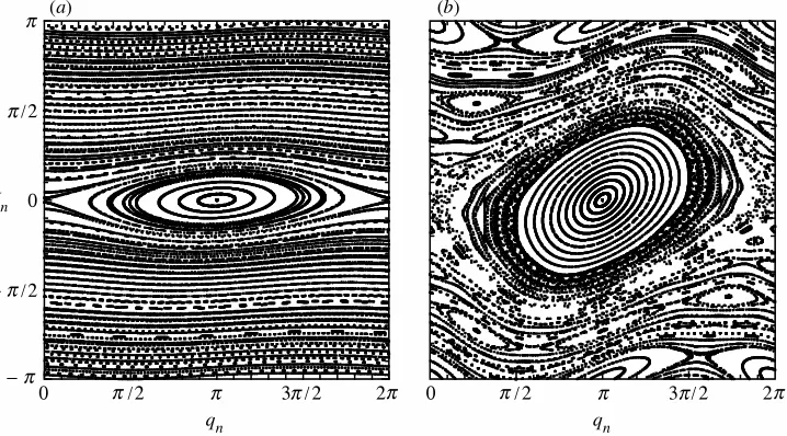
Figure 3. Trajectories in the standard map (1.1): (a)° = 0:1; (b) ° = 0:8. For small°, several features are apparent: there are ¯xed points (at (³; I) = (0;0) and (º;0)), periodic orbits and two types of quasi-periodic orbit|those that have a bounded range of³(in an island centred on (º;0)), and those for which³increases or decreases monotonically. For larger°, more islands are visible, as well as chaotic dynamics between the islands, and yet some quasi-periodic trajectories persist.

of spatially periodic patterns, it can be proved that this process, if carried to the limit, will indeed converge to a true solution. However, in the case of quasi-periodic behaviour, the corrections turn out not to be uniformly small, owing to the appear-ance of small numbers in the denominators, and convergence is called into question. This di±culty was faced ¯rst by Poincar¶e in the context of celestial mechanics in the late nineteenth century. In the absence of any gravitational interaction between planets, each planet in the Solar System orbits the Sun with its own period, and the system as a whole is quasi-periodic in time. Poincar¶e considered the question of whether or not the Solar System is quasi-periodic given the presence of weak interactions between the planets. Formally, the problem could be solved by pertur-bation theory, but Poincar¶e realized that small divisors called convergence of the perturbation series into question.

The small-divisor issue was resolved for this type of problem by Kolmogorov, Arnol’d & Moser (KAM) in the 1950s and 1960s, who showed under what circum-stances quasi-periodic behaviour would be found (see, for example, Moser 1973). To take an example, consider the so-called standard map:

In+ 1=In+°sin(³n); ³n+ 1=³n+In+ 1 mod 2º; (1.1)

which models a freely rotating pendulum in the absence of gravity, subjected to periodic impulsive forces. The map also models a chain of particles connected by springs and subjected to a sinusoidal potential (Aubry 1983). Here,nplays the role of time (or space in the particle model). When°= 0, all trajectories are of the form (³n; In) = (³0+nI0; I0) mod 2º, and are periodic with period q if I0=2º = p=q is

quasi-periodic orbits lie on horizontal lines (invariant curves) in the (³; I)-plane, but the lines are made up of individual periodic points in the ¯rst case, while a quasi-periodic orbit will eventually visit a neighbourhood of each point on the line. When°

is perturbed away from zero (see ¯gure 3a), the question is which of these families of trajectories will persist as invariant curves of the map? The essential content of the KAM theorem is that, for small enough perturbations, and for almost every irrational value of I0=2º, there will be an invariant curve close to the unperturbed invariant

curve, and the corresponding quasi-periodic trajectory survives the perturbation. The curves that persist are those that satisfy a Diophantine condition, that is, for which there are constantsK >0 and¯ >0 such thatI₀=2ºsatis¯es

¯ ¯ ¯ ¯

p_¡ I0

2ºq ¯ ¯ ¯ ¯

> K

(jp_j+jq_j)¯ (1.2)

for every pair of integerspandq, apart from (0;0). The exponent¯is an indication of the `irrationality’ ofI0=2º, so, for example, (

p

5¡1)=2 satis¯es (1.2) with¯= 1. In general, curves with smaller values of¯persist to larger values of the perturbation °. Invariant curves with rational values ofI0=2ºare immediately broken up into elliptic

and hyperbolic periodic points, with a web of chaotic trajectories near the hyperbolic equilibria (see ¯gure 3b).

KAM theory has been applied successfully to a variety of problems in which small divisors arise, for instance quasi-periodicity in the Solar System and in the dynam-ics of charged particles in tokamak magnetic ¯elds. However, the methods of KAM (based around canonical coordinate transformations) were developed for problems in which quasi-periodicity occurs in only one direction (time), whereas quasi-patterns are quasi-periodic in two spatial directions. For this reason, KAM theory is not applicable to quasi-patterns, at least not directly, and either the theory must be extended to cover this case, or alternative methods must be developed. In prin-ciple, similar issues arise in solid-state quasi-crystals, though the main theoretical approaches for these are developed around aperiodic Penrose tilings of the plane or three-dimensional space, and around projecting higher-dimensional periodic lattices down to three dimensions (Janot 1994), whereas a wave-based approach is more natural for the °uid dynamical quasi-patterns.

s |k_{| = 1}

|k|

k 12

k 1

(a) (b)

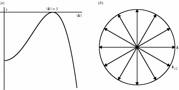
Figure 4. (a) Schematic growth (decay) rates of a mode ei ¢ _{, as a function of j}k_{jat·= 0.} Modes withjk_{j= 1 are marginally stable. (b) Twelve wavevectors on the circlej}k_{j= 1. Adding} equal amounts of 12 modes with these wavevectors (numberedk_1tok_{12) results in the synthetic} pattern in ¯gure 2c.

2. Model equations

One of the key mathematical questions concerning quasi-patterns is one ofexistence: do PDEs that model pattern-forming problems have solutions that are quasi-periodic in space, along the lines of the experimentally observed pattern in ¯gure 2a? Rather than try to answer this question in the context of a PDE that speci¯cally models the Faraday wave problem, it seems sensible to start with the simplest possible pattern-forming PDE: the Swift{Hohenberg equation (Swift & Hohenberg 1977). In fact, considering the Swift{Hohenberg equation is not such a simpli¯cation, since many pattern-forming problems can be cast into this form, or variations (Melbourne 1999). The simplest variant is

@U

@t =·U ¡(1 +r

2₎2_U¡U3_{: (2.1)}

The equation is posed on the plane, withx_{= (x; y)2R}2_{, andU(x; y; t)2Rsupposed}

to be bounded as (x; y)_{! 1}. The parameter · represents the force that will drive the pattern formation.

This PDE has a spatially uniform trivial solution U(x; y; t) = 0, and the stability of this solution can be investigated by linearizing (2.1). The linearized equation has wavelike solutions: U= est_eik¢x

, with growth rate s and wavevectork_{, with the}

growth rate related to · and _jk_{j by s=·¡(1¡ j}k_j2₎2_{. This relation is plotted in}

¯gure 4ain the case·= 0: with this value of·, all modes are damped (have negative growth rate) apart from those with wavenumber _jk_{j equal to 1. With · just above}

zero, modes with_jk_{jclose to 1 will grow, until the nonlinear term in (2.1) causes the}

amplitudes of these modes to saturate at a level related to the value of·.

degree of smallness is explicitly introduced as a small parameter ° _½ 1, and U is written in the form

U =°U1+°3U3+°5U5+¢ ¢ ¢ : (2.2)

The absence of even terms (°2_U

2) is because of the symmetry U ! ¡U in

equa-tion (2.1). The connecequa-tion between the small forcing · and the small parameter °

is made explicit by setting ·=°2_{. The expansion (2.2) is inserted into the Swift{}

Hohenberg equation (2.1) and like powers of° are collected together:

0 =°_L (U1) +°3(U1+L (U3)¡U13) +°5(U3+L (U5)¡3U12U3) +¢ ¢ ¢;

where, to make the presentation simpler, only steady patterns are considered. The linear di®erential operator L (U) is ¡(1 +r2₎2_U.

In order for this equation to be satis¯ed for all parameter values, the coe±cient of each power of°must separately be zero, and so the equation can be solved formally by considering each power of° in turn. The leading-order equation is

L (U1) = 0: (2.3)

The operator L acting on a mode eik¢x

yields ¡(1¡ jk_j2₎2_eik¢x

, which is zero only when _jk_{j= 1, so equation (2.3) has non-trivial solutions that are made up of}

lin-ear combinations of modes with wavevectors k _{on the unit circle. Any set of such}

wavevectors is possible at this level, but a natural choice to make when studying quasi-patterns is

U₁(x; y) =

12

X

j= 1

Ajei

k_j¢x

;

where the 12 vectors k_{1 to} k_{12 are equally spaced around the circle (¯gure 4b).}

This choice of modes is inspired by the evidence in the Fourier transforms of exper-imentally observed quasi-patterns (as in ¯gure 2b). In order for U to be real, the amplitudes must satisfy Aj+ 6= ¹Aj. Setting each Aj to the same real value results

in a quasi-pattern of the form depicted in ¯gure 2c. At third order in °, the equation to solve is

L (U3) =¡U1+U13=¡ 12

X

j= 1

Ajei

k_j¢x

+

12

X

j= 1 12

X

k= 1 12

X

l= 1

AjAkAlei(

k_j+ k_k+ k_l)¢x

: (2.4)

Notice thatU3

1 contains cubic interactions between the modes inU1, which take the

form of modes with all possible combinations of three of the 12 original wavevectors (allowing repeats). Some combinations (for example, k₁₊k₁₊k_{7 =} k_{1) lie on the}

unit circle, but most (k₁₊k₂₊k_{3) do not. Modes with di®erent wavevectors are}

orthogonal, so the coe±cients of each mode on the left and the right of equation (2.4) must be equal. In particular, the coe±cient of modes with wavevectors on the unit circle is zero on the left, since_L acting on such a mode is zero. Setting the coe±cient of (for example) eik₁¢x

to zero on the right-hand side results in an equation relating the amplitudes of the modes:

0 =A1¡3(jA1j2+ 2jA2j2+ 2jA3j2+ 2jA4j2+ 2jA5j2+ 2jA6j2)A1; (2.5)

solution is A1=¢ ¢ ¢=A12= 1=

p

33, and so, in terms of the original variables, the pattern is

U(x; y) =

r ·

33

12

X

j= 1

eik_j¢x

+_{¢ ¢ ¢}: (2.6)

This result suggests that the quasi-pattern solution is created when · increases through zero, with an amplitude proportional top·.

This might appear to be the end of the story: the amplitude of the quasi-pattern has been computed as a function of the driving force, and a little more e®ort leads to an estimate of the stability of the pattern. This kind of calculation has been carried out in a variety of situations, starting either from equations describing the Faraday wave experiment or other experiments, or just using considerations of the symmetry of the quasi-pattern. All these calculations result in amplitude equations similar to (2.5), and all su®er from two severe drawbacks.

The ¯rst drawback is that equation (2.5) determines only the amplitudes of the complex numbers Aj, and not their phase. In all, there are six free phases: two of these are ¯xed by considering resonances that occur at ¯fth order; two are genuinely free, and are associated with translating (but not changing) the pattern; and two phases (called phason modes) are not determined even by high-order resonances. In this context, the phason modes describe relative translations of two hexagonal sublattices generated byk_1,k_3, k_{5 and}k_2,k_4,k_{6, and may play a role in long-wave}

instabilities of the quasi-pattern (Echebarria & Riecke 2001). However, as they have a marked e®ect on the appearance of the pattern, they ought to be determined in a satisfactory theory without long-wave considerations.

The second drawback becomes apparent only when an attempt is made to compute higher-order corrections to the pattern. Returning to equation (2.4), all modes with wavevectors on the unit circle have already been taken into account by solving (2.5). The remaining modes all have wavevectors o® the unit circle (jk_{j 6= 1), and so the}

linear operator L can be inverted to ¯ndU₃:

U3 =¡

X

jkj+ kk+ klj6= 1

AjAkAl

(1_{¡ j}k_j+k_k+k_lj2₎2e

i(kj+ kk+ kl)¢x_;

since the operator L ¡1 _{acting on a mode e}ik¢x

yields ¡eik¢x₌

(1¡ jk_j2₎2_{, de¯ned as}

long asjk_{j 6= 1.}

However, if jk_{j is close to one, L} ¡1_(eik_¢x

) can be arbitrarily large. This does not pose di±culties for computing U3, but continuing the calculation to higher-order

results in combinations of vectors that can come arbitrarily close to the unit circle. Speci¯cally,U3 involves sums of three of the original 12 vectors, andUN will involve

integer combinations of up to N of the 12 vectors k_{1 to} k_{12. If the original choice}

100 101 102 103 104 105 N

10-10 10-8 10-6 10-4 10-2 100

(a) (b) (c)

(d)

||

k

|

1

|

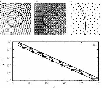
Figure 5. Positions of combinations of up toN of the original 12 vectors on the unit circle, with (a)N = 11, (b)N = 15; (c) detail of (b). The circle indicates the unit circle,jk_{j= 1, the} large dots are the original 12 wavevectors, and the small dots are integer combinations of these. Note how the density of points increases withN, and the proximity of points to the unit circle decreases withN. (d) Smallest non-zero distances from the unit circle jjk_{mj ¡1jas a function} of the total number of modes jm_{j=N. Stars mark distances calculated from equation (3.2),} and straight lines indicate the scalingN¡ 2_{. (After Rucklidge & Rucklidge (2003).)}

3. Small divisors

Does the smallness of the small divisors arising from inverting_L cause the sum (2.2)

for U(x; y; t) to diverge? To answer this question, the ¯rst stage is to derive a

Diophantine-like condition for integer combinations of up to N of the 12 original vectors on the unit circle (such combinations arising at orderN in the power series for U). It turns out that, for a given N, the smallest non-zero distance from the unit circle of a combination of N vectors is bounded above and below by a constant timesN¡2_.

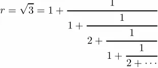
Table 1.Continued-fraction approximations tor=p3, as a function of the orderlof the truncation

l 0 1 2 3 4 5 6 7 8 9 10

r=p3 pl

ql 1 1 2 1 5 3 7 4 19 11 26 15 71 41 97 56 265 153 362 209 989 571

circle is of order N¡2_{, and the stars represent explicit combinations of wavevectors}

close to the unit circle, which were found as follows.

The vectors k_1;k_{2; : : : ;}k_{12 are labelled anticlockwise around the circle starting}

with k_{1 = (1;0), with}k_{j+ 6 = ¡}k_{j (¯gure 4b). Integer combinations ofN of these}

vectors can be written as

k_{m =}

12

X

j= 1

mjkj; with jmj= X

j

jmjj=N:

Including equal and opposite vectors, k_{j and} k_{j+ 6 will only increase N without}

coming any closer to the unit circle, so onlym1; : : : ; m6are considered, but these are

allowed to be negative. With this restriction, the squared length of a vectork_mis

jk_mj2 _=m2

1+m22+m23+m24+m25+m26

+m1m3+m2m4+m3m5+m4m6¡m5m1¡m6m2

+p3(m1m2+m2m3+m3m4+m4m5+m5m6¡m6m1):

This is of the form jk_mj2 _{= 1 +p¡rq, where r=}p_{3 is irrational and pand q are}

integers. Ifp_¡rqis close to zero (that is, ifris well approximated by the rationalp=q), thenjk_mj2 _{can come close to 1 (but can only be exactly 1 ifp=q= 0).}

It is clear that the theory of continued-fraction approximations of irrationals will be useful here. The continued-fraction expression forr=p3 is

r=p3 = 1 + 1

1 + 1

2 + 1

1 + 1 2 +_{¢ ¢ ¢}

:

That the value of this continued fraction isp3 can readily be shown by solving

r= 1 + 1

1 + 1

2 + (r_¡1)

= 3 + 2r 2 +r :

This equation can be rearranged to give r2_{¡3 = 0, sor=}p_{3 is the positive root.}

Since this irrational satis¯es a quadratic equation with integer coe±cients, p3 is called a quadratic irrational.

If the fraction is truncated afterlterms, the successive fractionspl=qlthat

irrationals (Hardy & Wright 1960) shows that K₁ q2 l < ¯ ¯ ¯ ¯ pl ql ¡r

¯ ¯ ¯ ¯

< K2 q2 l and ¯ ¯ ¯ ¯ pl ql ¡r

¯ ¯ ¯ ¯ < ¯ ¯ ¯ ¯ p

q ¡r

¯ ¯ ¯ ¯

; (3.1)

where K₁, K₂ are constants, and q is any integer satisfying 0 < q < ql. These

inequalities mean that the truncated continued-fraction expansions pl=ql approxi-mater well, but not too well, asl becomes large, and that ifpl=ql is the truncation of the continued-fraction approximation of an irrational r, no other fraction with a smaller denominator comes closer tor.

Apart from those vectors k_{m that fall exactly on the unit circle (which would}

havep=q= 0), the relations in (3.1) can be used to show thatjk_mj2_{can approach 1}

no faster than orderN¡2_:

jjk_mj2_¡1j> K N2;

where_jm_{j=N and K is a constant|this lower limit is shown as a straight line in}

¯gure 5d (see Rucklidge & Rucklidge (2003) for more details).

The order N¡2 _{rate of approach is indeed achieved by special combinations of}

vectors, which were found after a prolonged examination of the distances plotted in ¯gure 5d. Choosing

k_m=plk_{4+ (ql¡1)}k_{9+ (ql+ 1)}k_{11= (1; pl¡}p_{3ql); (3.2)}

with _jm_{j = N = pl+ 2ql and j}k_mj2_{¡1 = (pl¡}p_3ql)2_{. As N (or, equivalently, l}

or ql) increases, pl and ql are related by pl_¹p3ql+_O(1=ql), so ql = _O(N), and

jk_mj2_{¡1 = O(N}¡2_{). These particular choices of} k_{m are plotted on the graphs in}

¯gure 5d as stars. A little numerology suggests that pl+ 2ql = ql+ 2, so the values

ofN at which there is sudden drop injk_mj2_{¡1 areN = 3;4;11;15; : : :.}

In summary, given an integer N, the vector k_{m withj}m_{j=N that comes closest}

to the unit circle (without being on the unit circle) satis¯es

K

N2 6jjkmj 2

¡1_j6 K

0

N2;

for constants K and K0_{, for 12 equally spaced original vectors. The numerical}

evi-dence in ¯gure 5dsuggests values K = 0:56 andK0_{= 4:34.}

4. The question of convergence

The results of the previous two sections imply that whenk_{mis close to the unit circle,}

L ¡1_(eik ¢x_{) can be as large as a constant times N}4_eik ¢x_{, with N =}

jm_{j. This is}

so large that it clearly could lead to divergence of the power series (2.2) for U, particularly when nonlinear interactions of these large contributions are taken into account. This problem of small divisors is not just a feature of the particular Swift{ Hohenberg equation (2.1) used for illustration here, but arises in any calculation of the properties of quasi-patterns based on perturbation theory.

0 0.02 0.04

m

0.1 0.2

A(N)

N = 31

N = 29 N = 17 N = 13

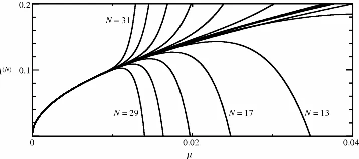
Figure 6. Amplitude A(N) _{as a function of·, for di®erent levels of truncation N = 1; : : : ;31.}

Increasing the order of truncation leads to graphs ofA(N)_{that diverge for·closer and closer to}

zero asN becomes larger. The amplitude has been scaled to remove a factor of 1=p33. (From Rucklidge & Rucklidge (2003).)

(33rd order in this case). If the series (2.2) is truncated to include powers of°up to and includingN + 2, the resulting expression for U(N) _{is of the form}

U(N)_=A(N) 12

X

j= 1

eikj¢x_{+ other modes;}

soA(1)₌p

·=33, from (2.6). The amplitudeA(N)_{of the basic quasi-pattern is shown}

as a function of · in ¯gure 6, for N = 1; : : : ;31. In this calculation, only modes with wavenumbers up to p5 were kept, to keep the total number of modes within manageable limits. Even so, there were more than 15 000 modes generated at the highest order|without this truncation, there would have been almost 2 000 000. Since the modes that were dropped from the calculation were the most heavily damped, their contribution to the total amplitude was quite small (of the order of 1%), and restricting the number of modes in this way had no e®ect on how close combinations of wavevectors could get to the unit circle.

It is clear in ¯gure 6 that, at each level of truncationN, the graph ofA(N)_against·

diverges at a value of·that decreases asN becomes larger. The value of·at which the sum up to orderN diverges is related to the smallest distance from the unit circle achieved by combinations of N of the 12 original wavevectors. Since this distance goes to zero asN increases, the sumA(N) _{will continue to diverge closer and closer}

to·= 0. In contrast, the equivalent calculation for spatially periodic patterns has a non-zero radius of convergence (Rucklidge & Rucklidge 2003).

5. Discussion and speculation

non-zero·, a low-order truncation may still give a useful asymptotic approximation of the quasi-pattern, assuming that the equations do have a quasi-pattern solution. It is on this basis that other researchers have proceeded.

There are two related issues at stake. First, existence: do pattern-forming PDEs (like the two-dimensional Swift{Hohenberg equation) have quasi-pattern solutions? A more general formulation of this question, using the Swift{Hohenberg equation as an example, becomes apparent by setting·=°2 _{in (2.1), scalingU by°and seeking}

a steady solution. The resulting equation can be written as

L (U) =°2(_¡U+U3);

which incidentally demonstrates that this is not a singularly perturbed problem. When ° = 0, any linear combination of waves with wavevectors on the unit circle solves this equation. The question is: which of these solutions persist to small but positive °? Current theory can so far only answer this question for those solutions that are spatially periodic. The limits on the rate of approach of wavevectors to the unit circle will play a central role in an eventual existence theory for quasi-patterns. The second issue is, given the small-divisor problem, are there methods that yield useful approximations to quasi-pattern solutions? Standard perturbation theory does not converge su±ciently rapidly (or slowly) to provide an answer unequivocally one way or the other. However, if quasi-pattern solutions exist, then the series ought to provide an asymptotic approximation to those solutions. Nonetheless, this approach will be left with di±culties, such as the undetermined phason modes, and so should not be regarded as a reliable way of computing properties of quasi-patterns.

What is needed is a method that converges more rapidly. Each order in the stan-dard theory gains a factor of°2 _{as well as large factors from any small divisors that}

arise. There are other methods, developed for proofs of KAM theory, that converge more rapidly, and these may be required for a rigorous treatment of quasi-patterns as well. The di®erence between the KAM situation and that of quasi-patterns is that in the KAM case, the solutions of interest are quasi-periodic in only one dimension (time), while in the second, quasi-patterns are quasi-periodic in two space directions. The problems that confront a proper mathematical theory of quasi-patterns are related to the di±culties that have arisen in other aspects of pattern formation: long-wave modulation of two-dimensional patterns, and the coexistence of spirals and spiral defect chaos with straight rolls. At the heart of this is the question of why, given that there is always a range of excited wavenumbers, spatially periodic pat-terns, characterized by asingle wavenumber, are often observed in spatially extended (e®ectively in¯nite) domains.

This last question has been answered rigorously in the context of one-dimensional patterns (stripes) in an in¯nite domain. Just above the onset of pattern formation, a range of wavenumbers close to _jk_{j = 1 are linearly unstable. Periodic patterns}

(a) (b) (c)

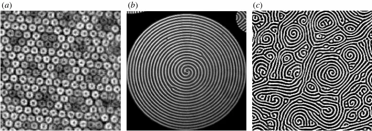
Figure 7. Other experimentally observed examples of pattern formation. (a) Spatially modulated hexagons in a two-frequency forced Faraday wave experiment. (Reproduced with permission from Arbell & Fineberg (2002). Copyright (2002) American Physical Society.) (b) Giant two-armed spiral in Rayleigh{B¶enard convection. (Reproduced with permission from Plappet al. (1998). Copyright (1998) American Physical Society.) (c) Spiral defect chaos in Rayleigh{B¶enard con-vection. (Reproduced with permission from Morris et al. (1993). Copyright (1993) American Physical Society.)

The di±culty in an in¯nite two-dimensional domain is that the linear stability problem is highly degenerate: patterns can form with any orientation, since all modes close to the circlejk_{j= 1 are linearly unstable. This leads to di±culties when trying to}

justify the use of two-dimensional versions of the Ginzburg{Landau equation, which only allow for a selection of these unstable modes. The modes that are not included in this approach could nonetheless be excited by nonlinear interactions between those that are included. It may be that the Ginzburg{Landau approach does provide a qualitatively correct description of numerical and laboratory experiments, but there is as yet no satisfactory justi¯cation for this. As a result, long wave modulations of two-dimensional patterns (as in, for example, ¯gure 7a) remain beyond reach. In particular, long-range changes in the orientation of a pattern are not captured by any current theory.

It seems unlikely, though perhaps possible, that a theory of two-dimensional pat-terns based on amplitudes of individual modes will be able to satisfy the two very dif-ferent requirements of mathematical rigour and of having su±cient °exibility to allow patterns of di®erent orientations, mixtures of (for example) squares and hexagons, quasi-patterns, defects, and so on. Allowing for all these possibilities would mean that amplitudes of all modes within a band around the circle_jk_{j= 1 would have to}

be included, and this would make the convergence problems discussed above much worse. There are patterns that do have modes with wavevectors of all orientations: giant spirals, for example (see ¯gure 7b). Even more puzzling and striking is spiral defect chaos (¯gure 7c), which has been observed in convection experiments with low-viscosity °uids. This pattern is made up of fragments of rolls and spirals, of size intermediate between the domain size and the scale of the pattern. This disordered state can occur close to the onset of convection and at the same parameters, the straight roll state is also stable. It is a challenge to see how amplitude-based models might be able to explain this phenomenon.

promis-ing way of understandpromis-ing pattern formation as a universal, problem-independent, phenomenon.

I am grateful to many people who have helped shape these ideas, in one way or another, over a period of several years. This research is supported by the Engineering and Physical Sciences Research Council.

References

Arbell, H. & Fineberg, J. 2002 Pattern formation in two-frequency forced parametric waves. Phys. Rev.E65, 036224.

Aubry, S. 1983 The twist map, the extended Frenkel{Kontorova model and the devil’s staircase. Physica D7, 240{258.

Cakmur, R. V., Egolf, D. A., Plapp, B. B. & Bodenschatz, E. 1997 Bistability and competition of spatiotemporally chaotic and ¯xed point attractors in Rayleigh{B¶enard convection.Phys. Rev. Lett.79, 1853{1856.

Echebarria, B. & Riecke, H. 2001 Sideband instabilities and defects of quasipatterns. Physica D158, 45{68.

Edwards, W. S. & Fauve, S. 1994 Patterns and quasi-patterns in the Faraday experiment. J. Fluid Mech.278, 123{148.

Golubitsky, M. & Stewart, I. 2002The symmetry perspective: from equilibrium to chaos in phase space and physical space. Basel: Birkhauser.

Hardy, G. H. & Wright, E. M. 1960An introduction to the theory of numbers, 4th edn. Oxford: Clarendon.

Janot, C. 1994Quasicrystals: a primer, 2nd edn. Oxford: Clarendon.

Levine, D. & Steinhardt, P. J. 1984 Quasicrystals: a new class of ordered structures.Phys. Rev. Lett.53, 2477{2480.

Melbourne, I. 1999 Steady-state bifurcation with Euclidean symmetry.Trans. Am. Math. Soc. 351, 1575{1603.

Morris, S. W., Bodenschatz, E., Cannell, D. S. & Ahlers, G. 1993 Spiral defect chaos in large aspect ratio Rayleigh{B¶enard convection.Phys. Rev. Lett.71, 2026{2029.

Moser, J. 1973Stable and random motions in dynamical systems. Princeton University Press. Plapp, B. B., Egolf, D. A., Bodenschatz, E. & Pesch, W. 1998 Dynamics and selection of giant

spirals in Rayleigh{B¶enard convection.Phys. Rev. Lett.81, 5334{5337.

Rucklidge, A. M. & Rucklidge, W. J. 2003 Convergence properties of the 8, 10 and 12 mode representations of quasipatterns.Physica D178, 62{82.

A U T H O R P R O F I L E

A. M. Rucklidge