Adriano Peron and Carla Piazza (Eds.):
Proceedings of the Fifth International Symposium on
Games, Automata, Logics and Formal Verification (GandALF 2014) EPTCS 161, 2014, pp. 60–73, doi:10.4204/EPTCS.161.8
c
Peter Faymonville and Martin Zimmermann This work is licensed under the
Creative Commons Attribution License. Peter Faymonville Martin Zimmermann
Reactive Systems Group, Saarland University, 66123 Saarbr¨ucken, Germany {faymonville, zimmermann}@react.uni-saarland.de
We introduce Parametric Linear Dynamic Logic (PLDL), which extends Linear Dynamic Logic (LDL) by temporal operators equipped with parameters that bound their scope. LDL was proposed as an extension of Linear Temporal Logic (LTL) that is able to express allω-regular specifications while still maintaining many of LTL’s desirable properties like an intuitive syntax and a translation into non-deterministic B¨uchi automata of exponential size. But LDL lacks capabilities to express timing constraints. By adding parameterized operators to LDL, we obtain a logic that is able to ex-press allω-regular properties and that subsumes parameterized extensions of LTL like Parametric LTL and PROMPT-LTL.
Our main technical contribution is a translation of PLDL formulas into non-deterministic B¨uchi word automata of exponential size via alternating automata. This yields a PSPACE model checking algorithm and a realizability algorithm with doubly-exponential running time. Furthermore, we give tight upper and lower bounds on optimal parameter values for both problems. These results show that PLDL model checking and realizability are not harder than LTL model checking and realizability.
1
Introduction
Linear temporal logic (LTL) is a popular specification language for the verification and synthesis of re-active systems. It provides semantic foundations for industrial logics like PSL [5]. LTL has a number of desirable properties contributing to its ongoing popularity: it does not rely on the use of variables, it has an intuitive syntax and thus gives a way for practitioners to write declarative and concise specifications. Furthermore, it is expressively equivalent to first-order logic over the natural numbers with successor and order [10] and enjoys an exponential compilation property: one can efficiently construct a language-equivalent non-deterministic B ¨uchi automaton of exponential size in the size of the specification. The exponential compilation property yields a PSPACE model checking algorithm and a 2EXPTIME algo-rithm for realizability. Both problems are complete for the respective classes.
Model checking of properties described in LTL or its practical descendants is routinely applied in industrial-sized applications, especially for hardware systems [2, 5]. Due to its complexity, the real-izability problem has not reached industrial acceptance (yet). First approaches used a determinization procedure forω-automata, which is notoriously hard to implement efficiently [16]. More recent algo-rithms for realizability follow a safraless construction [6, 7], which avoids explicitly constructing the deterministic automaton, and are showing promise on small examples.
Despite the desirable properties, two drawbacks of LTL remain and are tackled by different ap-proaches in the literature: first, LTL is not able to express allω-regular properties. For example, the property “p holds on every even step” (but may or may not hold on odd steps) is not expressible in LTL, but easily expressible as anω-regular expression. This drawback is a serious one, since the combination of regular properties and linear-time operators is common in hardware verification languages. Several
extensions of LTL [12, 20, 21] with regular expressions, finite automata, or grammar operators have been proposed as a remedy.
A second drawback of classic temporal logics like LTL is the inability to natively express timing constraints. The standard semantics are unable to enforce the fulfillment of eventualities within finite time bounds, e.g., it is impossible to require that requests are granted within a fixed, but arbitrary, amount of time. While it is possible to unroll an a-priori fixed bound for an eventuality into LTL, this requires prior knowledge of the system’s granularity and incurs a blow-up when translated to automata, and is thus considered impractical. A more practical way of fixing this drawback has been the purpose of a long line of work in parametric temporal logics, such as parametric LTL [1], PROMPT–LTL [11] and parametric metric interval temporal logic [9]. All of them add parameters to the temporal operators to express time bounds, and either test the existence of a global time bound, like PROMPT–LTL, or of individual bounds on the parameters, like parametric LTL.
Recently, the first drawback was revisited by De Giacomo and Vardi [4, 19] by introducing an extension of LTL called linear dynamic logic (LDL), which is as expressive as ω-regular languages. The syntax of LDL is inspired by propositional dynamic logic (PDL) [8], but the semantics follow linear-time logics. In PDL and LDL, programs are expressed by regular expressions with tests, and temporal requirements are specified by two basic modalities: hriϕ and [r]ϕ, stating thatϕ should hold at some position where r matches, or at all positions where r matches, respectively. The operators to specify regular expressions from propositional formulas are as follows: sequential composition (r1; r2),
nondeterministic choice (r1+r2), repetition (r∗), and test (ϕ?) of a temporal formula. On the level
of the temporal operators, conjunction and disjunction are allowed. The tests allow to check temporal properties within programs, and are needed to encode LTL into LDL.
As an example, the program “while q do a” with property p holding after the execution of the loop is expressed in PDL/LDL as follows:[(q? ; a)∗;¬q?]p. Intuitively, the loop condition q is tested on every
loop entry, the loop body a is executed/consumed until¬q holds, and then the post-condition p has to
hold. A request-response property (i.e., every request should eventually be followed by a response) can be formalized as follows:[tt∗](req→ htt∗iresp).
Both aforementioned drawbacks of LTL, the inability to express all ω-regular properties and the missing capability to specify timing constraints, have been tackled individually in a successful way in previous work, but not at the same time. Here, we propose a logic called PLDL that combines the expressivity of LDL with the parametricity of PLTL on infinite traces.
In PLDL, we are for example able to parameterize the eventuality of the request-response condition, denoted as[tt∗](req→ htt∗i≤xresp), which states that every request has to be followed by a response
within x steps. In the PLDL model checking problem, we determine whether there exists a valuation α(x)for x such that all paths of the system respond to requests withinα(x)steps. If we take the property as a specification for the PLDL realizability problem, and define req as input, resp as output, we compute whether there exists a winning strategy that adheres to a valuationα(x)and is able to ensure the delivery of responses to requests in a timely manner.
The main result of this paper is the translation of PLDL to alternating B ¨uchi automata. By an exten-sion of the alternating color technique of [11], and by very similar algorithms, we obtain the following results: PLDL model checking is PSPACE-complete and realizability is 2EXPTIME-complete. Thus, both problems are no harder than their corresponding variants for LTL. Finally, we give tight exponen-tial and doubly-exponenexponen-tial bounds on satisfying valuations for model checking and realizability.
2
PLDL
LetV be an infinite set of variables and let us fix a finite1set P of atomic propositions which we use to
build our formulas and to label transition systems in which we evaluate them. For a subset A∈2Pand a propositional formulaφ over P, we write A|=φ, if the variable valuation mapping elements in A to true and elements not in A to false satisfiesφ. The formulas of PLDL are given by the grammar
ϕ::=p| ¬p|ϕ∧ϕ|ϕ∨ϕ| hriϕ|[r]ϕ| hri≤zϕ|[r]≤zϕ r ::=φ|ϕ?|r+r|r ; r|r∗
where p∈P, z∈V, and whereφ stands for arbitrary propositional formulas over P. We use the
abbre-viationstt=p∨ ¬p andff=p∧ ¬p for some atomic proposition p. The regular expressions have two
types of atoms: propositional formulas φ over the atomic propositions and tests ϕ?, whereϕ is again a PLDL formula. Note that the semantics of the propositional atomφ differ from the semantics of the testφ?: the former consumes an input letter, while tests do not make progress on the word. This is why both types of atoms are allowed.
The set of subformulas ofϕis denoted by cl(ϕ). Note that regular expressions are not subformulas, but the formulas appearing in the tests are, e.g., we have cl(hp? ; qi≤xr) ={p,r,hp? ; qi≤xr}. The size|ϕ|
ofϕis the sum of|cl(ϕ)|and the sum of the lengths of the regular expressions appearing inϕ (counted with multiplicity). We define var♦(ϕ) ={z∈V | hri≤zψ∈cl(ϕ)}to be the set of variables
parameteriz-ing diamond operators inϕ, var(ϕ) ={z∈V |[r]≤zψ∈cl(ϕ)}to be the set of variables parameterizing
box operators inϕ, and set var(ϕ) =var♦(ϕ)∪var(ϕ). Usually, we will denote variables in var♦(ϕ)by
x and variables in var(ϕ)by y, ifϕis clear from the context. A formulaϕis variable-free, if var(ϕ) =/0. The semantics of PLDL are defined inductively with respect to anω-word w=w0w1w2· · · ∈(2P)ω,
a position n∈N, and a variable valuationα:V →Nvia
• (w,n,α)|=p if p∈wnand dually for¬p,
• (w,n,α)|=ψ0∧ψ1if(w,n,α)|=ψ0and(w,n,α)|=ψ1,
• (w,n,α)|=ψ0∨ψ1if(w,n,α)|=ψ0or(w,n,α)|=ψ1,
• (w,n,α)|=hriψ if there exists j∈Ns.t.(n,n+j)∈R(r,w,α)and(w,n+j,α)|=ψ,
• (w,n,α)|= [r]ψ if for all j∈Nwith(n,n+j)∈R(r,w,α)we have(w,n+j,α)|=ψ,
• (w,n,α)|=hri≤zψif there exists 0≤ j≤α(z)s.t.(n,n+j)∈R(r,w,α)and(w,n+j,α)|=ψ,
• (w,n,α)|= [r]≤zψ if for all 0≤ j≤α(z)with(n,n+j)∈R(r,w,α)we have(w,n+j,α)|=ψ.
Here, the relation R(r,w,α) ⊆N×Ncontains all pairs (m,n) such that wm· · ·wn−1 matches r (α is needed to evaluate tests in r, which might have parameterized subformulas) and is defined inductively by
• R(φ,w,α) ={(n,n+1)|wn|=φ}for propositionalφ,
• R(ψ?,w,α) ={(n,n)|(w,n,α)|=ψ},
• R(r0+r1,w,α) =R(r0,w,α)∪R(r1,w,α),
• R(r0; r1,w,α) ={(n0,n2)| ∃n1s.t.(n0,n1)∈R(r0,w,α)and(n1,n2)∈R(r1,w,α)}, and
• R(r∗,w,α) ={(n,n)|n∈N} ∪ {(n0,nk+1)| ∃n1, . . . ,nk s.t.(nj,nj+1)∈R(r,w,α)for all j≤k}.
We write(w,α)|=ϕ for(w,0,α)|=ϕ and say that w is a model ofϕ with respect toα.
Example 1.
• The formulaθ∞p:=[tt∗]htt∗ip expresses that p holds true infinitely often.
• In general, every PLTL formula [1] (and thus every LTL formula) can be translated into PLDL, e.g., F≤xp is expressible ashtt∗i≤xp and p U q ashp∗iq orhp∗qitt.
• The formula [tt∗](q→ h(tt;tt)∗pi) requires that every request (a position where q holds) is followed by a response (a position where p holds) after an even number of steps.
As usual for parameterized temporal logics, the use of variables has to be restricted: bounding dia-mond and box operators by the same variable leads to an undecidable satisfiability problem (cp. [1]).
Definition 1. A PLDL formulaϕis well-formed, if var♦(ϕ)∩var(ϕ) =/0.
In the following, we only consider well-formed formulas and drop the qualifier “well-formed”. We consider the following fragments of PLDL. Letϕ be a PLDL formula: ϕ is an LDL formula [4], ifϕ is variable-free, ϕ is a PLDL♦ formula, if var(ϕ) = /0, and ϕ is a PLDL formula, if var♦(ϕ) = /0. Every LDL, PLDL♦, and every PLDL formula is well-formed by definition. As satisfaction of LDL formulas is independent of variable valuations, we write(w,n)|=ϕand w|=ϕinstead of(w,n,α)|=ϕ and(w,α)|=ϕ, respectively, ifϕis an LDL formula.
LDL is as expressive asω-regular languages, which can be proven by a straightforward translation of ETLf [20], which expresses exactly theω-regular languages, into LDL.
Theorem 1 ([19]). For everyω-regular language L⊆(2P)ω there exists an effectively constructible LDL formulaϕsuch that L={w∈(2P)ω|w|=ϕ}.
Note that we define PLDL formulas to be in negation normal form. Nevertheless, a negation can be pushed to the atomic propositions using dualities allowing us to define the negation of a formula.
Lemma 1. For every PLDL formulaϕ there exists an efficiently constructible PLDL formula¬ϕ s.t.
1. (w,n,α)|=ϕif and only if(w,n,α)6|=¬ϕ,
2. |¬ϕ|=|ϕ|.
3. Ifϕis well-formed, then so is¬ϕ. and vice versa.
Proof. We construct¬ϕ by structural induction overϕ using the dualities of the operators:
• ¬(p) =¬p
• ¬(ϕ∧ψ) = (¬ϕ)∨(¬ψ)
• ¬(hriϕ) = [r]¬ϕ
• ¬(hri≤xϕ) = [r]≤x¬ϕ
• ¬(¬p) =p
• ¬(ϕ∨ψ) = (¬ϕ)∧(¬ψ)
• ¬([r]ϕ) =hri¬ϕ
• ¬([r]≤yϕ) =hri≤y¬ϕ
The latter two claims of Lemma 1 follow from the definition of¬ϕwhile the first one can be shown by a straightforward structural induction overϕ.
A simple, but very useful property of PLDL is the monotonicity of the parameterized operators: in-creasing (dein-creasing) the values of parameters bounding diamond (box) operators preserves satisfaction.
Lemma 2. Letϕbe a PLDL formula and letα andβ be variable valuations satisfyingβ(x)≥α(x)for every x∈var♦(ϕ)andβ(y)≤α(y)for every y∈var(ϕ). If(w,α)|=ϕ, then(w,β)|=ϕ.
Lemma 3. For every PLDL formulaϕ there is an efficiently constructible PLDL♦ formula ϕ′ of the
same size asϕsuch that
1. for everyα there is anα′such that for all w: if(w,α)|=ϕthen(w,α′)|=ϕ′, and
2. for everyα′there is anαsuch that for all w: if(w,α′)|=ϕ′then(w,α)|=ϕ.
Proof. We construct a single test ˆr such thatR(r,w,α)∩ {(n,n)|n∈N}=R(ˆr,w,α)for every w and
everyα, which suffices to prove the equivalence of[r]≤yψ and[ˆr]ψ provided we haveα(y) =0, which
is sufficient due to monotonicity. We apply the following rewriting rules (in the given order) to r:
1. Replace every subexpression of the form r′∗bytt?, until no longer applicable.
2. Replace every subexpression of the formφ; r′ or r′;φ byff? and replace every subexpression of the formφ+r′or r′+φby r′, whereφis a propositional formula, until no longer applicable.
3. Replace every subexpression of the formψ0?+ψ1? by(ψ0∨ψ1)? and replace every subexpression
of the formψ0? ;ψ1? by(ψ0∧ψ1)?, until no longer applicable.
After step 2, r contains no iterations and no propositional atoms unless the expression itself is one. In the former case, applying the last two rules yields a regular expression which is a single test, which we denote by ˆr. In the latter case, we define ˆr=ff?.
Each rewriting step preserves the intersectionR(r,w,α)∩ {(n,n)|n∈N}. As ˆr is a test, we conclude
R(r,w,α)∩{(n,n)|n∈N}=R(ˆr,w,α)for every w and everyα. Note that ˆr can be efficiently computed
from r and is of the same size as r. Now, replace every subformula[r]≤yψ ofϕ by[ˆr]ψ and denote the
formula obtained byϕ′, which is a PLDL♦formula that is efficiently constructible and of the same size. Given anα, we defineα0 byα0(z) =α(z), if z∈var♦(ϕ)andα0(z) =0 otherwise. If(w,α)|=ϕ,
then(w,α0)|=ϕ due to monotonicity. By construction ofϕ′, we also have(w,α0)|=ϕ′. On the other
hand, if(w,α′)|=ϕ′, then(w,α′
0)|=ϕ′as well, whereα0′ is defined as above. By construction ofϕ′, we
conclude(w,α0)|=ϕ.
2.1 The Alternating Color Technique and LDLcp
In this subsection, we repeat the alternating color technique, which was introduced by Kupferman et al. to solve the model checking and the realizability problem for PROMPT–LTL, amongst others. Let
p∈/P be a fresh proposition and define P′=2P∪{p}. We think of words in(2P′)ω as colorings of words
in (2P)ω, i.e., w′ ∈(2P′)ω is a coloring of w∈(2P)ω, if we have w
n′∩P=wn for every position n.
Furthermore, n is a changepoint, if n=0 or if the truth value of p differs at positions n−1 and n. A block is a maximal infix that has exactly one changepoint, which is at the first position of the infix. By maximality, this implies that the first position after a block is a changepoint. Let k≥1. We say that w′is
k-bounded, if every block has length at most k, which implies that w′has infinitely many changepoints. Dually, w′ is k-spaced, if it has infinitely many changepoints and every block has length at least k.
The alternating color technique replaces a parameterized diamond operatorhri≤xψ by an
unparam-eterized one that requires the formulaψ to be satisfied within at most one color change. To this end, we introduce a changepoint-bounded variant h·icp of the diamond operator. Since we need the dual
operator[·]cpto allow for negation via dualization, we introduce it here as well. We define
• (w,n,α)|=hricpψ′if there exists a j∈Ns.t.(n,n+j)∈R(r,w,α), wn· · ·wn+j−1contains at most
one changepoint, and(w,n+j,α)|=ψ, and
• (w,n,α)|= [r]cpψ′if for all j∈Nwith(n,n+j)∈R(r,w,α)and where wn· · ·wn+j−1contains at
We denote the logic obtained by disallowing parameterized operators, but allowing changepoint-bounded operators, by LDLcp. Note that the semantics of LDLcp formulas are independent of
vari-able valuations. Hence, we drop them from our notation for the satisfaction relations|=andR. Also,
Lemma 1 can be extended to LDLcpby adding the rules¬(hricpψ) = [r]cp¬ψand¬([r]cpψ) =hricp¬ψ
to the proof.
Now, we are ready to introduce the alternating color technique. Given a PLDL♦formulaϕ, let rel(ϕ) be the formula obtained by inductively replacing every subformulahri≤xψ byhrel(r)icprel(ψ), i.e., we
replace the parameterized diamond operator by a changepoint-bounded one. Note that this replacement is also performed in the regular expressions, i.e., rel(r)is the regular expression obtained by applying the replacement to every testψ′? in r.
Given a PLDL♦formulaϕlet c(ϕ) =rel(ϕ)∧θ∞p∧θ∞¬p (cf. Example 1), which is an LDLcp
for-mula and only linearly larger thanϕ. On k-bounded and k-spaced colorings of w there is an equivalence betweenϕ and c(ϕ). The proof is similar to the original one [11].
Lemma 4 (cp. Lemma 2.1 of [11]). Letϕ be a PLDL♦formula and let w∈(2P)ω.
1. If(w,α)|=ϕ, then w′|=c(ϕ)for every k-spaced coloring w′of w, where k=maxx∈var(ϕ)α(x). 2. Let k∈N. If w′ is a k-bounded coloring of w with w′|=c(ϕ), then(w,α)|=ϕ, whereα(x) =2k
for every x.
3
From LDL
cpto Alternating B ¨uchi Automata
In this section, we show how to translate LDLcp formulas into alternating B ¨uchi word automata of
linear size using an inductive bottom-up approach. These automata allow us to use automata-based constructions to solve the model checking and the realizability problem for PLDL via the alternating color technique which links PLDL and LDLcp.
An alternating B ¨uchi automatonA= (Q,Σ,q0,δ,F)consists of a finite set Q of states, an alphabetΣ, an initial state q0∈Q, a transition functionδ: Q×Σ→B+(Q), and a set F⊆Q of accepting states.
Here,B+(Q)denotes the set of positive boolean combinations over Q, which contains in particular the
formulastt(true) and ff(false). A run ofAon w=w0w1w2· · · ∈Σω is a directed graphρ = (V,E) with V ⊆Q×Nand((q,n),(q′,n′))∈E implies n′=n+1 such that the following two conditions are satisfied: (q0,0)∈V and for all(q,n)∈V : Succρ(q,n)|=δ(q,wn). Here Succρ(q,n)denotes the set of
successors of(q,n)inρprojected to Q. A runρ is accepting if all infinite paths (projected to Q) through ρvisit F infinitely often. The language L(A)contains all w∈Σω that have an accepting run ofA.
Theorem 2. For every LDLcpformulaϕ, there is an alternating B¨uchi automatonAϕ with linearly many
states (in|ϕ|) such that L(Aϕ) ={w∈(2P′)ω|w|=ϕ}.
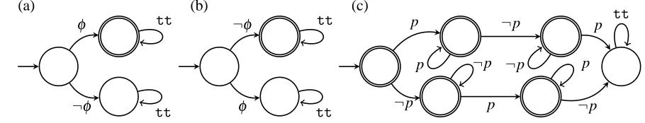
To prove the theorem, we inductively construct automataAψ for every subformulaψ∈cl(ϕ) satisfy-ing L(Aψ) ={w∈(2P′)ω |w|=ψ}. The automata for atomic formulas are straightforward and depicted
in Figure 1(a) and (b). To improve readability, we allow propositional formulas over P′ as transition labels: the formulaφ stands for all sets A∈2P′ with A|=φ. Furthermore, given automataAψ
0 andAψ1,
using a standard construction, we can build the automatonAψ
0∨ψ1 by taking the disjoint union of the two
automata, adding a new initial state q0withδ(q0,A) =δ0(q00,A)∨δ1(q10,A). Here, qi0is the initial state
andδi is the transition function ofAψ
i. The automatonAψ0∧ψ1 is defined similarly, the only difference
beingδ(q0,A) =δ0(q00,A)∧δ1(q10,A).
(a) (b) (c) φ ¬φ tt tt ¬φ φ tt tt p ¬p
p ¬p
[image:7.612.76.531.69.156.2]¬p p p ¬p ¬p p tt
Figure 1: The automataAp(a),A¬p(b), andAcp(c), which tracks color changepoints.
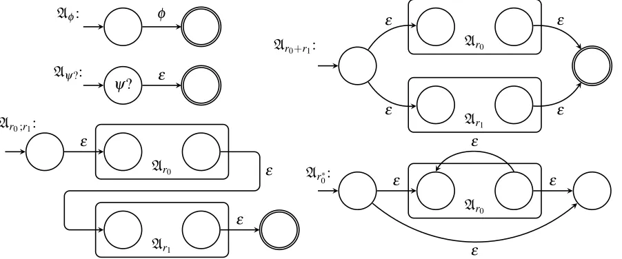
defining the transition function, but we label states at which the test has to be executed by this test. We use the Thompson construction [18] to turn r into Ar, i.e., we obtain an ε-NFA. Then, we show how to combineAr with the automatonAψ and the automataAψ
1, . . . ,Aψk, whereψ1?, . . . ,ψk? are the test occurring in r. Theε-transitions introduced by the Thompson construction are then removed, since alternating automata do not allow them. During this process, we also ensure that the transition relation takes tests into account by introducing universal transitions that lead from a state marked withψj? into
the corresponding automatonAψ j.
Formally, an ε-NFA with markings A= (Q,Σ,q0,δ,C,m) consists of a finite set Q of states, an alphabetΣ, an initial state q0∈Q, a transition functionδ: Q×Σ∪ {ε} →2Q, a set C of final states (C,
since we use them to concatenate automata), and a partial marking function m, which assigns to some states q∈Q an LDLcpformula m(q). We write q−→a q′, if q′∈δ(q,a)for a∈Σ∪ {ε}. Anε-pathπfrom
q to q′inAris a sequenceπ=q1· · ·qkof k≥1 states with q=q1−→ · · ·ε −→ε qk=q′. The set of allε-paths from q to q′is denoted byΠ(q,q′). Let m(π) ={m(qi)|1≤i≤k}be the set of markings visited byπ.
A run ofAon w0· · ·wn−1∈Σ∗is a sequence q0q1· · ·qnsuch that for every i in the range 0≤i≤n−1 there is a state q′i reachable from qi via anε-path πi and with qi+1∈δ(q′i,wi). The run is accepting if
there is a q′n∈C reachable via anε-pathπnfrom qn. This slightly unusual definition (but equivalent to
the standard one) simplifies our reasoning below. Also, the definition is oblivious to the marking. We begin by defining the automatonArby induction over the structure of r as depicted in Figure 2. Note that the automata we construct have no outgoing edges leaving the unique final state and that we mark some states with testsψj? (denoted by labeling states with the test).
Lemma 5. Let w=w0w1w2· · · ∈(2P
′
)ω and let w0· · ·wn−1be a (possibly empty, if n=0) prefix of w. The following two statements are equivalent:
1. Arhas an accepting run q0q1· · ·qnon w0· · ·wn−1withε-pathsπifor i in the range 0≤i≤n such
that wiwi+1wi+2· · · |=Vm(πi)for every i. 2. (0,n)∈R(r,w).
Fixψ and r (with tests ψ1?, . . . ,ψk?) and letAr= (Qr,2P
′
,qr0,δr,Cr,m),A
ψ = (Q′,2P′,q′0,δ′,F′),
andAψ j = (Q
j,2P′,qj
0,δj,Fj)for j=1, . . . ,k be the corresponding automata, which we assume to have
pairwise disjoint sets of states. Next, we show how to constructAhriψ,A[r]ψ,Ahri
cpψ, andA[r]cpψ. We begin withhriψ: we defineAhriψ = (Qr∪Q′∪Q1∪ · · · ∪Qk,2P′,qr
0,δ,F1∪ · · · ∪Fk)with
δ(q,A) =
δ′(q,A) if q∈Q′,
δj(q,A) if q∈Qj,
W
q′∈Qr\CrWπ∈Π(q,q′)Wp∈δr(q′,A)(p∧Vψ
j∈m(π)δ
j(qj 0,A))
∨ if q∈Qr.
W
q′∈CrWπ∈Π(q,q′)(δ′(q′0,A)∧Vψ
j∈m(π)δ
Aφ:
Aψ?:
Ar0+r1:
Ar0;r
1:
Ar∗
0:
φ
ψ? ε
[image:8.612.85.536.66.254.2]Ar0 Ar1 ε ε ε ε Ar0 Ar1 ε ε ε Ar0 ε ε ε ε
Figure 2: The inductive definition ofArvia the Thompson construction.
So, Ahriψ is the union of the automata for the regular expression, the tests, and forψ with a modified transition function. The transitions of the automataAψ and Aψ
j are left unchanged and the transition function for states in Qr is obtained by removing ε-transitions. First consider the upper disjunct: it ranges disjunctively over all non-final states p that are reachable via an initialε-path and an A-transition in the end. To account for the tests visited during theε-path (but not the test at p), we add conjunctively transitions that lead into the corresponding automata. The lower disjunct is similar, but ranges over paths that end in a final state. Since we concatenate the automatonArwith the automatonAψ, all edges leading into final states ofArare rerouted to the initial state ofAψ. The tests along theε-path are accounted for as in the first case. Finally, note that Qrdoes not contain any (B ¨uchi) accepting states, i.e., every accepting
run on w has to leave Qr after a finite number of transitions. Since this is only possible via transitions that would leadArinto a final state, this ensures the existence of a position n such that(0,n)∈R(r,w).
The definition of A[r]ψ is dual, i.e., we have to use automata A¬ψ j = (Q
j,2P′,qj
0,δj,Fj) for j=
1, . . . ,k for the negated tests andε-transitions are removed in a universal manner. Formally, we define A[r]ψ = (Qr∪Q′∪Q1∪ · · · ∪Qk,2P′,qr
0,δ,Qr∪F1∪ · · · ∪Fk)where
δ(q,A) =
δ′(q,A) if q∈Q′,
δj(q,A) if q∈Qj,
V
q′∈Qr\CrVπ∈Π(q,q′)Vp∈δr(q′,A)(p∨Wψ
j∈m(π)δ
j(qj 0,A))
∧ if q∈Qr.
V
q′∈CrVπ∈Π(q,q′)(δ′(q′0,A)∨Wψ
j∈m(π)δ
j(qj 0,A))
Note that we add Qrto the (B ¨uchi) accepting states, since a run on w might stay in Qrforever, as it has to consider all positions n with(0,n)∈R(r,w).
For the changepoint-bounded operators, we have to modifyAr to make it count color changes. Let Acp= (Qcp,2P′,qcp
0 ,δcp,Ccp)be the DFA depicted in Figure 1(c). We define the product ofArand Acp
as ˆAr= (Qˆr,2P′,qˆr
0,δˆr,Cˆr,mˆ)where ˆQr=Qr×Qcp, ˆqr0= (qr0,q cp 0 ),
δ((q,q′),A) =
(
{(p,δcp(q′,A))|p∈δr(q,A)} if A6=ε,
ˆ
Cr=Cr×Ccp, and ˆm(q,q′) =m(q). Using this, we defineAhri
cpψ as we definedAhriψ, but using ˆAr instead ofAr. Similarly,A[r]cpψ is defined asA[r]ψ, but using ˆArinstead ofAr.
Proof of Theorem 2. First, we consider the size ofAϕ. Boolean operations add one state while a temporal operator with regular expression r adds a number of states that is linear in the size of r (which is its length), even when we take the intersection with the automaton checking for color changes. Note that we do not need to complement the automataAψ
j to obtainA¬ψj, instead we rely on Lemma 1. Hence, the size ofAϕ is linear in the size ofϕ. It remains to prove L(Aϕ) ={w∈(2P′)ω |w|=ϕ}by induction over the structure ofϕ. The induction start for atomic formulas and the induction step for disjunction and conjunction are trivial, hence it remains to consider the temporal operators.
Considerhriψ. If w|=hriψ, then there exists a position n such that wnwn+1wn+2· · · |=ψ and(0,n)∈ R(r,w). Hence, there is a run ofAron w0· · ·wn−1such that the tests visited during the run are satisfied by the appropriate suffixes of w. Thus, applying the induction hypothesis yields accepting runs of the test automata on these suffixes. Furthermore, there is an accepting run ofAψ on wnwn+1wn+2· · ·, again by induction hypothesis. These runs can be “glued” together to build an accepting run ofAhriψ on w.
For the other direction, consider an accepting run ρ ofAhriψ on w. Let n≥0 be the last level of ρ that contains a state from Qr. Such a level has to exist since states in Qr are not accepting and they have no incoming edges from states of the automata Aψ and Aψ
j, but the initial state of Ahriψ is in
Qr. Furthermore, Ahriψ is non-deterministic and complete when restricted to states in Qr\Cr. Hence, we can extract an accepting run ofAr fromρ on w0· · ·wn−1that satisfies additionally the requirements formulated in Statement 1 of Lemma 5, due to the transitions into the test automata and an application of the induction hypothesis. Hence, we have (0,n)∈R(r,w). Furthermore, from the remainder of ρ (levels greater or equal to n) we can extract an accepting run of Aψ on wnwn+1wn+2· · ·. Hence,
wnwn+1wn+2· · · |=ψ by induction hypothesis. Altogether, we conclude w|=hriψ.
The case for[r]ψ is dual, while the cases for the changepoint-bounded operatorshricpψ and[r]cpψ
are analogous, using the fact thatAcponly accepts words which have at most one changepoint.
Note that the size ofAϕ is linear in|ϕ|, but it is not clear that it can be computed in polynomial time in|ϕ|, since the transition functions of subautomata of the form Ahriψ contain disjunctions that range over the set of ε-paths. Here, it suffices to consider paths that do not contain a state twice, but even this restriction still allows for an exponential number of different paths. Fortunately, we do not need to computeAϕ in polynomial time. It suffices to do it in polynomial space, which is sufficient for the applications in the next sections, which is clearly possible.
Furthermore, using standard constructions (e.g., [13, 15]), we can turn the alternating B ¨uchi au-tomaton Aϕ into a non-deterministic B ¨uchi automaton of exponential size and a deterministic parity automaton2 of doubly-exponential size with linearly many colors.
4
Model Checking
In this section, we consider the PLDL model checking problem. A (P-labeled) transition systemS =
(S,s0,E, ℓ)consists of a finite set S of states, an initial state s0, a (left-)total edge relation E ⊆S×S,
and a labeling ℓ: S→2P. An initial path through S is a sequence π =s0s1s2· · · of states satisfying
(sn,sn+1)∈E for every n. Its trace is defined as tr(π) =ℓ(s0)ℓ(s1)ℓ(s2)· · ·. We say thatS satisfies a
2The states of a parity automaton are colored byΩ: Q→N. It accepts a word w, if it has a run q
0q1q2· · · on w such that
PLDL formulaϕwith respect to a variable valuationα, if we have(tr(π),α)|=ϕfor every initial pathπ ofS. The model checking problem asks, given a transition systemS and a formulaϕ, to determine
whetherS satisfiesϕwith respect to some variable valuationα.
Theorem 3. The PLDL model checking problem is PSPACE-complete.
To solve the PLDL model checking problem, we first notice that we can restrict ourselves to PLDL♦ formulas. Letϕ and ϕ′ be due defined as in Lemma 3. Then,S satisfiesϕ with respect to some α if
and only ifS satisfiesϕ′ with respect to someα′.
Our algorithm is similar to the one presented for PROMPT–LTL in [11] and uses the alternating color technique. Recall that p∈/P is the fresh atomic proposition used to specify the coloring and induces the
blocks, maximal infixes with its unique changepoint at the first position. Let G= (V,E,v0, ℓ,F)denote
a colored B ¨uchi graph consisting of a finite directed graph(V,E), an initial vertex v0, a labeling
func-tion ℓ: V →2{p} labeling vertices by p or not, and a set F⊆V of accepting states. A path v0v1v2· · ·
through G is pumpable, if all its blocks have at least one state that appears twice in this block. Further-more, the path is fair, if it visits F infinitely often. The pumpable non-emptiness problem asks, given a colored B ¨uchi graph G, whether it has a pumpable fair path starting in the initial state.
Theorem 4 ([11]). The pumpable non-emptiness problem for colored B¨uchi graphs is NLOGSPACE -complete and can be solved in linear time.
The following lemma reduces the PLDL♦model checking problem to the pumpable non-emptiness problem for colored B ¨uchi graphs of exponential size. Given a non-deterministic B ¨uchi automatonA= (Q,2P∪{p},q0,∆,F)recognizing the models of¬rel(ϕ)∧θ∞p∧θ∞¬p (note that rel(ϕ)is negated) and a
transition systemS = (S,s0,E, ℓ), we define the productA×S to be the colored B ¨uchi graph
A×S = (Q×S×2{p},E′,(q0,s0,/0), ℓ′,F×S×2{p})
where((q,s,C),(q′,s′,C′))∈E′if and only if(s,s′)∈E and q′∈δ(q, ℓ(s)∪C), and whereℓ′(q,s,C) =C.
Each initial path(q0,s0,C0)(q1,s1,C1)(q2,s2,C2)· · · through the productA×S induces a coloring
(L(s0)∪C0)(L(s1)∪C1)(L(s2)∪C2)· · · of the trace of the path s0s1s2· · · through S. Furthermore, q0q1q2· · · is a run ofAon the coloring.
Lemma 6 (cp. Lemma 4.2 of [11]). S does not satisfyϕwith respect to anyαif and only ifA×S has a pumpable fair path.
Proof. Letϕ not be satisfied byS with respect to anyα, i.e., for everyα there exists an initial pathπ
through S such that(tr(π),α)6|=ϕ. Pickα∗such that α∗(x) =2· |Q| · |S|+1 and letπ∗ be the
cor-responding path. Applying Lemma 4.2 yields w6|=c(ϕ) for every|Q| · |S|-bounded coloring of tr(π∗). Now, consider the unique |Q| · |S|-bounded and|Q| · |S|-spaced coloring w of tr(π∗) that starts with p not holding true in the first position. As argued above, w6|=c(ϕ), and we have w|=θ∞p∧θ∞¬p, as w is
bounded. Hence, w|=¬rel(ϕ)∧θ∞p∧θ∞¬p, i.e., there is an accepting run q0q1q2· · · ofAin w. This
suf-fices to show that(q0,π0,w0∩ {p})(q1,π1,w1∩ {p})(q1,π1,w2∩ {p})· · ·is a pumpable fair path through A×S, since every block has length greater than|Q| · |S|. This implies the existence of a repeated state
in every block, since there are exactly|Q| · |S|vertices of each color.
Now, letA×S contain a pumpable fair path(q0,s0,C0)(q1,s1,C1)(q2,s2,C2)· · ·, fix some arbitrary α, and define k=maxx∈var♦ϕα(x). There is a repetition of a vertex ofA×S in every block, each of
which can be pumped k times. This path is still fair and induces a coloring w′k of a trace wkof an initial
path ofS. Since the run encoded in the first components is an accepting one on w′
k, we conclude that
Towards a contradiction assume we have(w,α)|=ϕ. Applying Lemma 4.1 yields w′|=c(ϕ), which contradicts¬c(ϕ). Hence, for everyα we have constructed a path ofS whose trace does not satisfyϕ
with respect toα, i.e.,S does not satisfyϕwith respect to anyα.
We can deduce an upper bound on valuations that satisfy a formula in a given transition system.
Corollary 1. If there is a variable valuation such that S satisfies ϕ, then there is also one that is bounded exponentially in|ϕ|and linearly in the number of states ofS.
Proof. LetS satisfy ϕ with respect toα, but not with the valuation α∗ with α∗(x) =2· |Q| · |S|+1.
In the preceding proof, we constructed a pumpable fair path inA×S starting from this assumption.
This contradicts Lemma 6, sinceS satisfyingϕ with respect toα is equivalent toA×S not having a
pumpable fair path. Since 2· |Q| · |S|+1 is exponential in|ϕ|and linear in|S|, the result follows.
A matching lower bound of 2ncan be proven by implementing a binary counter with n bits using a formula of polynomial size in n. This holds already true for PROMPT–LTL, as noted in [11].
It remains to prove the main result of this section: PLDL model checking is PSPACE-complete.
Proof of Theorem 3. PSPACE-hardness follows directly from the PSPACE-hardness of the LTL model checking problem [17], as LTL is a fragment of PLDL.
The following is a PSPACE algorithm: constructA×S and check whether it contains a pumpable
fair path, which is correct due to Lemma 6. Since the search for such a path can be implemented on-the-fly without having to construct the full product [11], it can be implemented using polynomial space.
5
Realizability
In this section, we consider the realizability problem for PLDL. Throughout the section, we fix a parti-tion(I,O)of the set of atomic propositions P. An instance of the PLDL realizability problem is given by a PLDL formulaϕ (over P) and the problem is to decide whether Player O has a winning strategy in the following game, played in rounds n∈N: in each round n, Player I picks a subset in ⊆I and then Player O picks a subset on⊆O. Player O wins the play with respect to a variable valuationα, if
((i0∪o0)(i1∪o1)(i2∪o2)· · ·,α)|=ϕ.
Formally, a strategy for Player O is a mapping σ: (2I)∗→2O and a play ρ =i
0o0i1o1i2o2· · · is
consistent with σ, if we have on=σ(i0· · ·in) for every n. We call (i0∪o0)(i1∪o1)(i2∪o2)· · · the
outcome ofρ, denoted by outcome(ρ). We say that a strategyσ for Player I is winning with respect to a variable valuationα, if we have(outcome(ρ),α)|=ϕfor every playρ that is consistent withσ. The PLDL realizability problem asks for a given PLDL formulaϕ, whether Player O has a winning strategy with respect to some variable valuation, i.e., there is a singleα such that every outcome satisfiesϕwith respect toα. If this is the case, then we say thatσ realizesϕand thus thatϕis realizable.
We show the PLDL realizability problem to be 2EXPTIME-complete: hardness follows easily from the 2EXPTIME-completeness of the LTL realizability problem, which is a special case of the PLDL realizability problem. Membership in 2EXPTIME on the other hand is shown by a reduction to the realizability problem forω-regular specifications.
It is well-known thatω-regular specifications are realizable by finite-state transducers (if they are realizable at all) [3]. A transducer T = (Q,Σ,Γ,q0,δ,τ) consists of a finite set Q of states, an input
alphabetΣ, an output alphabet Γ, an initial state q0, a transition functionδ: Q×Σ→Q, and a output
where δ∗ is defined as usual: δ∗(ε) =q0 and δ∗(wv) =δ(δ∗(w),v). To implement a strategy by a
transducer, we useΣ=2IandΓ=2O. Then, we say that the strategyσ= fT is finite-state. The size of
σ is the number of states ofT. The following proof is analogous to the one for PROMPT–LTL [11]. Theorem 5. The PLDL realizability problem is 2EXPTIME-complete.
When proving membership in 2EXPTIME, we restrict ourselves without loss of generality to PLDL♦ formulas, as this special case is sufficient as shown in Lemma 3. First, we use the alternating color tech-nique to show that the PLDL♦ realizability problem is reducible to the realizability problem for speci-fications in LDLcp. When considering the LDLcp realizability problem, we add the fresh proposition p
used to specify the coloring to O, i.e., Player O is in charge of determining the color of each position.
Lemma 7 (cp. Lemma 3.1 of [11]). A PLDL♦ formulaϕ over I and O is realizable if and only if the LDLcpformula c(ϕ)over I and O∪ {p}is realizable.
Proof. Letϕ be realizable, i.e., there is a winning strategyσ:(2I)+→2Ofor Player O with respect to
someα. Now, consider the strategyσ′:(2I)+→2O∪{p}defined by
σ′(i
0· · ·in−1) = (
σ(i0· · ·in−1) if n mod 2k<k, σ(i0· · ·in−1)∪ {p} otherwise,
where k=maxx∈var♦(ϕ)α(x). We show thatσ
′ realizes c(ϕ). To this end, letρ′=i
0o0i1o1i2o2· · · be
a play that is consistent withσ′. Then, ρ=i0(o0\ {p})i1(o1\ {p})i2(o2\ {p})· · · is by construction
consistent withσ, i.e.,(outcome(ρ),α)|=ϕ. Asρ′is a k-spaced p-coloring ofρ, we deduceρ′|=c(ϕ) by applying Lemma 4.1. Hence,σ′realizes c(ϕ).
Now, assume c(ϕ)is realized by σ′: (2I)+→2O∪{p}, which we can assume to be finite-state, say
it is implemented byT with n states. We first show that every outcome that is consistent with σ′ is n+1-bounded. Such an outcome satisfies c(ϕ) and has therefore infinitely many changepoints. Now, assume it has a block of length strictly greater than n+1, say between changepoints at positions i and j. Let q0q1q2· · · be the states reached during the run ofT on the projection ofρto 2I. Then, there are two
positions i′and j′satisfying i≤i′<j′< j in the block such that qi′=qj′. Hence, q0· · ·qi′−1(qi′· · ·qj′−1)ω
is also a run ofT. However, the output generated by this run has only finitely many changepoints, since
the output at the states qi′, . . . ,qj′−1 coincides when restricted to {p}. This contradicts the fact that
T implements a winning strategy, which implies in particular that every output has infinitely many
changepoints, as required by the conjunctθ∞p∧θ∞¬pof c(ϕ). Hence,ρis(n+1)-bounded.
Now, consider the strategyσ:(2I)+→2Odefined byσ(i
0· · ·in−1) =σ′(i0· · ·in−1)∩O. By
defini-tion, for every playρ consistent with σ, there is a(n+1)-bounded p-coloring of ρ that is consistent withσ′. Hence, applying Lemma 4.2 yields(ρ,β)|=ρ, whereβ(x) =2n+2. Hence,σ realizesϕwith respect toβ. Note thatσ is also finite-state and of the same size asσ′.
Proof of Theorem 5. As already mentioned above, 2EXPTIME-hardness of the LDL realizability prob-lem follows immediately from the 2EXPTIME-hardness of the LTL realizability problem [14], as LTL is a fragment of PLDL.
Now, consider membership and recall that we have argued that it is sufficient to consider PLDL♦. Thus, letϕbe a PLDL♦formula. By Lemma 7 we know that it is sufficient to consider the realizability of c(ϕ). LetA= (Q,2I∪O∪{p},q0,δ,Ω)be a deterministic parity automaton recognizing the models of
c(ϕ). We turnAinto a parity gameG such that Player 1 winsG from some dedicated initial vertex if and
i⊆I and Player O picks a subset o⊆O, which in turn triggers the (deterministic) update of the state
stored in the vertices. Finally, we define the coloringΩA of the arena viaΩA(q) =ΩA(q,i) =Ω(q).
It is straightforward to show that Player O has a winning strategy from q0in the parity game(A,ΩA)
if and only if c(ϕ)(and thus ϕ) is realizable. Furthermore, if Player 1 has a winning strategy, thenA
can be turned into a transducer implementing a strategy that realizes c(ϕ)using V as set of states. Note that|V|is doubly-exponential in|ϕ|, if we assume that I and O are restricted to propositions appearing inϕ. As the parity game is of doubly-exponential size and has linearly many colors, we can solve it in doubly-exponential time in the size ofϕ. This concludes the proof.
Also, we obtain a doubly-exponential upper bound on a variable valuation that allows to realize a given formula. A matching lower bound already holds for PLTL [22].
Corollary 2. If a PLDL♦formulaϕis realizable with respect to someα, then it is realizable with respect
to someα that is bounded doubly-exponentially in|ϕ|.
Proof. Ifϕ is realizable, then so is c(ϕ). Using the construction proving the right-to-left implication of Lemma 7, we obtain thatϕis realizable with respect to someα that is bounded by 2n+2, where n is the size of a transducer implementing the strategy that realizes c(ϕ). We have seen in the proof of Theorem 5 that the size of such a transducer is at most doubly-exponential in|c(ϕ)|, which is only linearly larger than|ϕ|. The result follows.
6
Conclusion
We introduced Parametric Linear Dynamic Logic, which extends Linear Dynamic Logic by temporal operators equipped with parameters that bound their scope, similarly to Parametric Linear Temporal Logic, which extends Linear Temporal Logic by parameterized temporal operators. Here, the model checking problem asks for a valuation of the parameters such that the formula is satisfied with respect to this valuation on every path of the transition system. Realizability is defined in the same spirit.
We showed PLDL model checking to be complete for PSPACE and the realizability problem to be complete for 2EXPTIME, just as for LTL. Thus, in a sense, PLDL is not harder than LTL. Finally, we were able to give tight exponential respectively doubly-exponential bounds on the optimal valuations for model checking and realizability.
We did not consider the assume-guarantee model checking problem here, but the algorithm solving the problem for PROMPT–LTL presented in [11] should be adaptable to PLDL as well. Another open problem concerns the computation of optimal valuations for PLDL♦and PLDLformulas. By exhaus-tive search within the bounds mentioned above, one can determine the optima. We expect this to be possible in polynomial space for model checking and in triply exponential space for realizability, which is similar to the situation for PLTL [1, 22]. Note that it is an open question whether optimal valuations for PLTL realizability can be determined in doubly-exponential time.
References
[1] Rajeev Alur, Kousha Etessami, Salvatore La Torre & Doron Peled (2001): Parametric Temporal Logic for
“Model Measuring”.ACM Trans. Comput. Log.2(3), pp. 388–407, doi:10.1145/377978.377990. [2] Roy Armoni, Limor Fix, Alon Flaisher, Rob Gerth, Boris Ginsburg, Tomer Kanza, Avner Landver, Sela
Logic: A New Temporal Property-Specification Language. In Joost-Pieter Katoen & Perdita Stevens, editors:
TACAS,LNCS2280, Springer, pp. 296–211, doi:10.1007/3-540-46002-0_21.
[3] J. Richard B¨uchi & Lawrence H. Landweber (1969): Solving Sequential Conditions by Finite-State Strategies.
Trans. Amer. Math. Soc.138, pp. pp. 295–311, doi:10.2307/1994916.
[4] Giuseppe De Giacomo & Moshe Y. Vardi (2013): Linear Temporal Logic and Linear Dynamic Logic on
Finite Traces. In Francesca Rossi, editor:IJCAI, IJCAI/AAAI. Available athttp://www.aaai.org/ocs/ index.php/IJCAI/IJCAI13/paper/view/6997.
[5] C. Eisner & D. Fisman (2006): A Practical Introduction to PSL. Integrated Circuits and Systems, Springer, doi:10.1007/978-0-387-36123-9.
[6] Emmanuel Filiot, Naiyong Jin & Jean-Franc¸ois Raskin (2011): Antichains and compositional algorithms for
LTL synthesis.Formal Methods in System Design39(3), pp. 261–296, doi:10.1007/s10703-011-0115-3. [7] Bernd Finkbeiner & Sven Schewe (2013): Bounded Synthesis. STTT15(5-6), pp. 519–539, doi:10.1007/
s10009-012-0228-z.
[8] Michael J. Fischer & Richard E. Ladner (1979): Propositional Dynamic Logic of Regular Programs.Journal
of Computer and System Sciences18(2), pp. 194 – 211, doi:10.1016/0022-0000(79)90046-1.
[9] Barbara Di Giampaolo, Salvatore La Torre & Margherita Napoli (2010): Parametric Metric Interval
Tem-poral Logic. In Adrian Horia Dediu, Henning Fernau & Carlos Mart´ın-Vide, editors: LATA,LNCS6031, Springer, pp. 249–260, doi:10.1007/978-3-642-13089-2_21.
[10] Hans W. Kamp (1968): Tense Logic and the Theory of Linear Order. Ph.D. thesis, Computer Science Department, University of California at Los Angeles, USA.
[11] Orna Kupferman, Nir Piterman & Moshe Y. Vardi (2009): From Liveness to Promptness.Formal Methods in
System Design34(2), pp. 83–103, doi:10.1007/s10703-009-0067-z.
[12] Martin Leucker & C´esar S´anchez (2007): Regular Linear Temporal Logic. In Cliff Jones, Zhiming Liu & Jim Woodcock, editors: ICTAC’07,LNCS4711, Springer-Verlag, Macau, China, pp. 291–305, doi:10. 1007/978-3-540-75292-9_20.
[13] Satoru Miyano & Takeshi Hayashi (1984): Alternating Finite Automata onω-Words. Theor. Comput. Sci.
32, pp. 321–330, doi:10.1016/0304-3975(84)90049-5.
[14] Amir Pnueli & Roni Rosner (1989): On the Synthesis of an Asynchronous Reactive Module. In Giorgio Ausiello, Mariangiola Dezani-Ciancaglini & Simona Ronchi Della Rocca, editors: ICALP,LNCS 372, Springer, pp. 652–671, doi:10.1007/BFb0035790.
[15] Sven Schewe (2009): Tighter Bounds for the Determinisation of B¨uchi Automata. In Luca de Alfaro, editor:
FOSSACS,LNCS5504, Springer, pp. 167–181, doi:10.1007/978-3-642-00596-1_13.
[16] Christoph Schulte Althoff, Wolfgang Thomas & Nico Wallmeier (2006): Observations on Determinization
of B¨uchi Automata.Theor. Comput. Sci.363(2), pp. 224 – 233, doi:10.1016/j.tcs.2006.07.026. [17] A. Prasad Sistla & Edmund M. Clarke (1985): The Complexity of Propositional Linear Temporal Logics. J.
ACM32(3), pp. 733–749, doi:10.1145/3828.3837.
[18] Ken Thompson (1968): Programming Techniques: Regular Expression Search Algorithm. Commun. ACM
11(6), pp. 419–422, doi:10.1145/363347.363387.
[19] Moshe Y. Vardi (2011): The Rise and Fall of LTL. In Giovanna D’Agostino & Salvatore La Torre, editors:
GandALF,EPTCS54, doi:10.4204/EPTCS.54. Invited presentation.
[20] Moshe Y. Vardi & Pierre Wolper (1994): Reasoning About Infinite Computations. Inf. Comput.115(1), pp. 1–37, doi:10.1006/inco.1994.1092.
[21] Pierre Wolper (1983): Temporal Logic Can be More Expressive. Information and Control56(1–2), pp. 72 – 99, doi:10.1016/S0019-9958(83)80051-5.