Exploiting correlogram structure for robust speech recognition with multiple speech sources

This is a repository copy of Exploiting correlogram structure for robust speech recognition with multiple speech sources .

White Rose Research Online URL for this paper: http://eprints.whiterose.ac.uk/3531/

Article:

Ma, N., Green, P., Barker, J. et al. (1 more author) (2007) Exploiting correlogram structure for robust speech recognition with multiple speech sources. Speech Communication, 49 (12). pp. 874-891. ISSN 0167-6393

https://doi.org/10.1016/j.specom.2007.05.003

[email protected] https://eprints.whiterose.ac.uk/

Reuse

Unless indicated otherwise, fulltext items are protected by copyright with all rights reserved. The copyright exception in section 29 of the Copyright, Designs and Patents Act 1988 allows the making of a single copy solely for the purpose of non-commercial research or private study within the limits of fair dealing. The publisher or other rights-holder may allow further reproduction and re-use of this version - refer to the White Rose Research Online record for this item. Where records identify the publisher as the copyright holder, users can verify any specific terms of use on the publisher’s website.

Takedown

If you consider content in White Rose Research Online to be in breach of UK law, please notify us by

promoting access to White Rose research papers

White Rose Research Online

Universities of Leeds, Sheffield and York

http://eprints.whiterose.ac.uk/

This is an author produced version of a paper published in Speech

Communication.

White Rose Research Online URL for this paper: http://eprints.whiterose.ac.uk/3531/

Published paper

Ma, N., Green, P., Barker, J. and Coy, A. (2007) Exploiting correlogram structure for robust speech recognition with multiple speech sources, Speech

Exploiting correlogram structure for robust

speech recognition with multiple speech

sources

Ning Ma

∗

, Phil Green, Jon Barker, Andr´

e Coy

Department of Computer Science, University of Sheffield, Regent Court, 211

Portobello Street, Sheffield, S1 4DP, UK

Abstract

se-quences. The paper presents evaluations based on artificially mixed simultaneous speech utterances. A coherence-measuring experiment is first reported which quan-tifies the consistency of the identified fragments with a single source. The system is then evaluated in a speech recognition task and compared to a conventional frag-ment generation approach. Results show that the proposed system produces more coherent fragments over different conditions, which results in significantly better recognition accuracy.

Key words: Speech separation, Robust speech recognition, Multiple pitch tracking,

Computational auditory scene analysis, Correlogram, Speech fragment decoding

1 Introduction

In realistic listening conditions, speech is often corrupted by competing sound

sources. The presence of acoustic interference can cause the quality or the

in-telligibility of speech to degrade; the performance in automatic speech

recog-nition (ASR) often drops dramatically. Many systems have been proposed to

separate noise from speech using cues from multiple sensors, e.g. blind source

separation by independent component analysis (Parra and Spence, 2000), but

separating and recognising speech in single-channel signals, the problem

con-sidered in this article, still remains a challenging problem. Human listeners,

however, are adept at recognising target speech in such noisy conditions,

mak-ing use of cues such as pitch continuity, spacial location, and speakmak-ing rate

∗ _{Corresponding author. Tel.: +44 114 222 1878, fax: +44 114 222 1810.}

Email addresses: [email protected] (Ning Ma),[email protected]

(Phil Green),[email protected] (Jon Barker), [email protected]

(Cooke and Ellis, 2001). They are able to effectively extract target audio

streams from monaural acoustic mixtures with little effort, e.g. listening to

speech/music mixtures on a mono radio program. It is believed that there

are processes in the auditory system that segregate the acoustic evidence into

perceptual streams based on their characteristics, allowing listeners to

selec-tively attend to whatever stream is of interest at the time (Bregman, 1990;

Cooke and Ellis, 2001). This offers an alternative to techniques which require

the noise to be effectively removed from the speech, e.g. spectral subtraction

based methods (Lim and Oppenheim, 1979), and allows the noise to be treated

as streams that can be ignored while the target speech is attended to.

This ability of listeners has motivated extensive research into the perceptual

segregation of sound sources and has resulted in much theoretical and

ex-perimental work inauditory scene analysis(ASA) (Bregman, 1990). Auditory

scene analysis addresses the problem of how the auditory system segregates the

mixture of sound reaching the ears into packages of acoustic evidence in which

each package is likely to have been produced from a single source of sound.

The analysis process, described by Bregman (1990), is interactively governed

by ‘primitive’ bottom-up grouping rules, which are innate constraints driven

by the incoming acoustic data and the physics of sound, and ‘schema-based’

top-down constraints, which employ the knowledge of familiar patterns that

have been learnt from complex acoustic environments. Computational

audi-tory scene analysis (CASA) aims to develop computational models of ASA.

Many researchers have proposed automatic sound separation systems based

on the known principles of human hearing and have achieved some success

(Brown and Cooke, 1994; Wang and Brown, 1999; Ellis, 1999). A good review

1.1 Correlogram-based CASA models

One important representation of auditory temporal activity that combine both

spectral and temporal information is the autocorrelogram (ACG). The

auto-correlogram, or simplycorrelogram, is a three-dimensional volumetric function,

mapping a frequency channel of an auditory periphery model, temporal

auto-correlation delay (or lag), and time to the amount of periodic energy in that

channel at that delay and time. Correlograms are normally sampled across

time to produce a series of two-dimensional graphs, in which frequency and

autocorrelation delay are displayed on orthogonal axes. Fig. 1 shows three

correlograms of a clean speech signal uttered by a female speaker, taken at

time frames of 300 ms, 700 ms and 2100 ms. Each correlogram has been

nor-malised and plotted as an image for illustration. The periodicity of sound is

well represented in the correlogram. If the original sound contains a signal that

is approximately periodic, such as voiced speech, then each frequency channel

excited by that signal will have a high similarity to itself delayed by the period

of repetition. The ACG frequency channels also all respond to the

fundamen-tal frequency (F0) and this can be emphasised by summing the ACG over

all frequency channels, producing a ‘summary ACG’ (see the bottom panel in

Fig. 1). The position of the largest peak in the summary ACG corresponds to

the pitch of the periodic sound source. Primarily because it is well-suited to

detecting signal periodicity, the correlogram is widely considered as the

pre-ferred computational representation of early sound processing in the auditory

system.

The correlogram was first suggested as a model for pitch perception by

sub-T = 2100 ms

0.0 2.5 5.0 7.5 10.0 12.5 15 0.5

1

Autocorrelation Delay (ms) T = 700 ms

0.0 2.5 5.0 7.5 10.0 12.5 15 0.5

1

Autocorrelation Delay (ms)

C e n tr eF re q u e n c y( H z )

T = 300 ms

50 395 1246 3255 8000

0.0 2.5 5.0 7.5 10.0 12.5 15 0.5

1

Autocorrelation Delay (ms)

Fig. 1. Three correlograms of a clean speech signal uttered by a female speaker, taken at time frame 300, 700 and 2100 ms, respectively. Each correlogram has been

normalised and plotted as an image. A corresponding summary ACG is shown at

the bottom of each correlogram.

band periodicity detection was discussed. The model was then reintroduced

by Slaney and Lyon (1990), among others (e.g. (Meddis and Hewitt, 1991)),

as a computational approach to pitch detection. Slaney and Lyon employed

the correlogram computed from the output of a cochlear model to model how

humans perceive pitch. The pitch was estimated based on locating the peaks in

the summary correlogram. The ACG model has subsequently been extended

as a popular mechanism for segregating concurrent periodic sounds and the

primary methods have been based on inspection of the summary correlogram.

Assmann and Summerfield (1990) reported a place-time model on a

concur-rent vowel segregation task. The model estimated the pitch of each vowel as

corresponding to the autocorrelation delays with the two largest peaks in the

summary correlogram. Meddis and Hewitt (1992) proposed a residual-driven

approach. They first selected the largest peak in the summary ACG, the

channels that respond to this F0 were grouped and removed from the

cor-relogram. The rest of the channels were integrated together and the largest

peak in the residue corresponds to the F0 of a second (and weaker) source.

Recently, neural oscillator models have been successful at providing accounts

of the interaction of cue combinations, such as common onset and proximity

(Brown and Cooke, 1994; Wang and Brown, 1999), in which the summary

correlogram model was also employed as a front end.

One limitation of the methods which are based on the summary correlogram

is that when speech is corrupted by competing sounds, locating peaks in the

summary is often difficult. The position of the largest peak in the summary

would not always correspond to the pitch of the target speech and peaks

indi-cating pitches of different sound sources may be correlated. Another limitation

is that these models cannot account for the effect of harmonic components of

the weaker source being dominated by the stronger source, where all

correlo-gram channels will be assigned to the stronger source (de Cheveign´e, 1993).

To address these limitations, Coy and Barker (2005) proposed to keep the

four largest peaks in the summary ACG as pitch candidates for each time

frame and then employed a multi-pitch tracker to form smooth pitch tracks

from these candidates. Frequency channels that respond to pitch values in the

same pitch track are grouped together. By keeping multiple pitch candidates

they show that better sound segregation can be achieved. However, their

sys-tem relies on a robust multipitch tracker and keeping an arbitrary number of

pitch candidates is not effective when dealing with different competing sources.

The summary ACG is not the only way to reveal pitch information. The

methods based on the summary ACG discard the rich representation of the

Visually there are clear pitch-related ‘dendritic structures’ in the correlogram.

The ‘dendrites’ are tree-like structures whose stems are centred on the delay

of multiple pitch periods across frequency channels. Slaney and Lyon (1990)

discussed this dendritic structure in their perceptual pitch detector. They

con-volved the correlogram with an operator to emphasise the structure before

in-tegrating all ACG channels together. Summerfield et al. (1990) also proposed a

convolution-based strategy for the separation of concurrent synthesised vowels

with F0 not harmonically related in the correlogram. By locating the dendritic

structure in the correlogram they demonstrated that multiple fundamentals

can be recognised.

1.2 Linking CASA with speech recognition systems

The success of CASA has inspired research into developing a new

genera-tion of automatic speech recognigenera-tion systems for natural listening condigenera-tions

where competing sounds are often present. In these adverse conditions not all

the acoustic evidence from the target source will be recovered. One successful

approach to this problem is ‘missing data ASR’ (Cooke et al., 2001), which

adapts the conventional probabilistic formalism of ASR to deal with the

‘miss-ing data’. The miss‘miss-ing data approach assumes that some acoustic data in the

mixture will remain uncorrupted and can be identified as reliable evidence for

recognition. Cooke et al. (1997) demonstrated that recognition can indeed be

based on a small amount (10% or less) of the original time-frequency ‘pixels’

if they can be correctly identified.

The limitation of the missing data approach is that accurate identification of

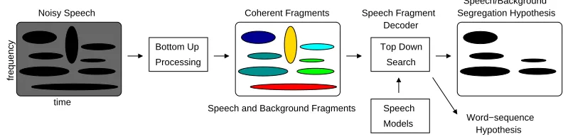
Speech Fragment Decoder

Speech Models Search Top Down

Word−sequence Hypothesis

frequency

time

Noisy Speech Segregation Hypothesis

Speech/Background

Processing Bottom Up

Coherent Fragments

Speech and Background Fragments

Fig. 2. An overview of the speech fragment decoding system (after Barker et al. (2005)). Bottom-up processes are employed to identify spectro-temporal regions

where each region is likely to have originated from a single source (coherent

frag-ments). A top-down search with access to speech models is then used to search for

the most likely combination of fragment labelling and speech model sequence.

is poor if the ‘missing data’ is not correctly identified. There is evidence that

listeners make use of both primitive and schema-based constraints when

per-ceiving speech signals (Bregman, 1990). Barker et al. (2005) proposed a Speech

Fragment Decoding (SFD) technique which treats segregation and recognition

as coupled problems. Primitive grouping processes exploit common

character-istics to identify sound evidence arising from a single source. Top-down search

utilises acoustic models of target speech to find the best acoustic combinations

which jointly explain the observation sequence without deciding the identity

of different sources. The SFD technique therefore provides a bridge that links

auditory scene analysis models with conventional speech recognition systems.

An overview of the SFD system is provided in Fig. 2.

1.3 Summary of the paper

In this article we are concerned with the use of primitive CASA models to

address the problem of separating and recognising speech in monaural acoustic

correlogram structure is exploited to separate a spectrogram representation

of the acoustic mixture into spectro-temporal regions such that the acoustic

evidence in each region is likely to have originated from a single source of

sound. These regions are referred to as ‘coherent fragments’ in this study.

Some of these fragments will arise from the target speech source while others

may arise from noise sources. These coherent fragments are passed to the

speech fragment decoder to identify the best subset of fragments as well as

the word sequence that best matches the target speech models. We evaluate

the system using a challenging simultaneous speech recognition task1_.

The remainder of this article is organised as follows: in the next section, the

overall structure of our system is briefly reviewed. Section 3 describes the

tech-niques used to integrate spectral components in each frame based on the ACG.

Section 4 presents methods which produce coherent fragments. Section 5

in-troduces a confidence map to soften the discrete decision of assigning a pixel to

a fragment. In Section 6 we evaluate the system and discuss the experimental

results. Section 7 concludes and presents future research directions.

2 System Overview

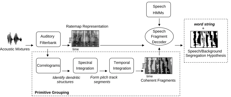
Fig. 3 shows the schematic diagram of our system. The input to the system is a

mixture of target speech and interfering sounds, sampled at a rate of 25 kHz. In

the first stage of the system, cochlear frequency analysis is simulated by a bank

of 64 overlapping bandpass Gammatone filters, with centre frequencies spaced

uniformly on the equivalent rectangular bandwidth (ERB) scale (Glasberg

Decoder Speech Fragment

Primitive Grouping

Auditory Filterbank

Integration Spectral

Integration

Speech/Background Segregation Hypothesis

+

Correlograms

structures segments Form pitch track

Speech HMMs

word string

Coherent Fragments Acoustic Mixtures time

freq

freq

time

Temporal

Identify dendritic

Ratemap Representation

Fig. 3.Schematic diagram of the proposed system.

and Moore, 1990) between 50 Hz and 8000 Hz. Gammatone filter modelling

is a physiologically motivated strategy to mimic the structure of peripheral

auditory processing stage (Cooke, 1991). The gains of the filters are chosen to

reflect the transfer function of the outer and middle ears. Having more filters

(e.g. 128) can offer a higher frequency resolution but bring more computational

cost. The output of each filter is then half-wave rectified.

The digital implementation of the Gammatone filter employed here was based

on the implementation of Cooke (1991) using the impulse invariant

transfor-mation. The sound is first multiplied by a complex exponential e−jωt _{at the}

desired centre frequency ω, then filtered with a baseband Gammatone filter,

and finally shifted back to the centre frequency region. The cost of computing

the complex exponential e−jωt _{for each sound sample t is a significant part of}

the overall computation. In our implementation, the exponential computation

is transformed into simple multiplication to reduce the cost by rearranging

e−jωt _to

The terme−jω _{can be pre-computed ande}−jω(t−1) _{is the result of the previous}

samplet−1. Therefore only one complex exponential calculation is needed for

the first sample and for the rest of samples the exponentials can be computed

by simple multiplication. Experiments showed that using this implementation

the Gammatone computation speed can be increased by a factor of 4.

Spectral features are then computed in order to employ the ‘speech fragment

decoder’ (Barker et al., 2005). The instantaneous Hilbert envelope is computed

at the output of each Gammatone filter. This is smoothed by a first-order

low-pass filter with an 8 ms time constant, sampled at 10 ms intervals, and finally

log-compressed to give an approximation to the auditory nerve firing rate –

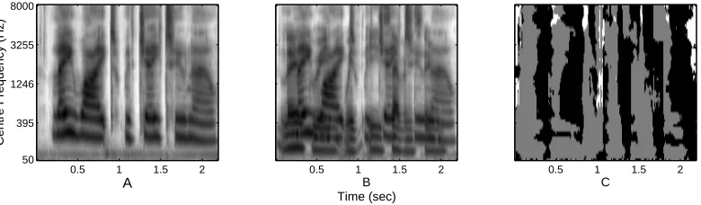
a ‘ratemap’ (Brown and Cooke, 1994). Fig. 4 gives an example of a ratemap

representation2_{, for (A) a female utterance ‘lay white with j 2 now’, and (B)}

the same utterance artificially mixed with a male utterance ‘lay green with e

7 soon’, with a target-to-masker ratio (TMR) of 0 dB. Panel (C) shows the

‘oracle’ segmentation, obtained by making use of the pre-mix clean signals.

Dark grey represents pixels where the value in the mixture is closer to that in

the target female speech; light grey represents pixels where the mixture value

is closer to that in the male speech; white pixels represent low energy regions.

These representations are called ‘missing data masks’.

The output of the auditory filterbank is also used to generate the

correlo-grams. A running short-time autocorrelation is computed on the output of

each cochlear filter, using a 30 ms Hann window. At a given time step t, the

2 _{All examples used in this study are utterances from the GRID corpus (Cooke}

A

Centre Frequency (Hz)

0.5 1 1.5 2 50

395 1246 3255 8000

B Time (sec)

0.5 1 1.5 2

C

0.5 1 1.5 2

Fig. 4. (A) A ‘ratemap’ representation for the utterance ‘lay white with j 2 now’ (target, female) without added masker. (B) Ratemap for the same utterance plus

‘lay green with e 7 soon’ (masker, male) with a TMR of 0 dB. (C) The ‘oracle’

segmentation: dark grey - the value in the mixture is close to that in the target

female speech; light grey - the mixture value is close to that in the male speech;

white pixels - low energy regions.

autocorrelation A(i, t, τ) for channeli with a time lag τ is given by

A(i, τ, t) =

K_X−1

k=0

g(i, t+k)w(k)g(i, t+k−τ)w(k−τ) (2)

where g is the output of the Gammatone filterbank and w is a local Hann

window of width K time steps. Here K = 750 corresponding to a window

width of 30 ms. The autocorrelation can be implemented using the efficient fast

Fourier transform (FFT), but has the disadvantage that longer autocorrelation

delays have attenuated correlation owing to the narrowing of the effective

window. We therefore use a scaled form of Eq. (2) with a normalisation factor

to compensate for the effect:

A(i, τ, t) = 1

K−τ

K_X−1

k=0

g(i, t+k)w(k)g(i, t+k−τ)w(k−τ) (3)

The autocorrelation delay τ is computed from 0 to L −1 samples, where

L = 375 corresponding a maximum delay of 15 ms. This is appropriate for

below 66.7 Hz. We compute the correlograms with the same frame shift as

when computing the ratemap features (10 ms), hence each one-dimensional

(frequency) ratemap frame has a corresponding two-dimensional (frequency

and autocorrelation delay) correlogram frame.

In the stage of spectral integration the dendritic structure is exploited in

the correlogram domain to segregate each frame of the mixture into spectral

groups, such that the partial spectra in each group is entirely due to a single

sound source in that frame. In the next stage local pitch estimates are

com-puted for each group and a multipitch tracker links these pitch estimates to

produce smooth pitch tracks. Spectral groups are integrated temporally based

on these pitch tracks. The processes separate the spectro-temporal

represen-tation of the acoustic mixture into a set of coherent fragments, which are then

employed in the ‘speech fragment decoder’, together with clean speech models,

to perform automatic speech recognition.

3 Spectral integration based on the ACG

3.1 The dendritic ACG structure

For a periodic sound source all autocorrelation channels respond to F0 (i.e.

the energy reaches a peak at the same frequency), forming vertical stems in

the correlogram centred on the delays corresponding to multiple pitch periods.

Meanwhile, because each filter channel also actively responds to the harmonic

component that is closest to its centre frequency (CF), the filtered signal in

each channel tends to repeat itself at an interval of approximately 1/CF, giving

Centre Frequency (Hz)

Clean female speech

50 395 1246 3255 8000

0.0 2.5 5.0 7.5 10.0 12.5 15 0.5

1

Autocorrelation Delay (ms)

Centre Frequency (Hz)

Female speech mixed with male speech

50 395 1246 3255 8000

0.0 2.5 5.0 7.5 10.0 12.5 15 0.5

1

Autocorrelation Delay (ms)

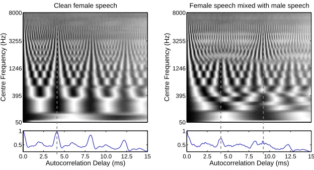
Fig. 5. A comparison of correlograms in clean and noisy conditions. Left – a cor-relogram and its summary of clean female speech, taken at time frame 60; right –

taken at the same frame when the female speech is mixed with male speech at a

TMR of 0 dB. The dendritic structures that correspond to theF_{0of different speech}

sources are marked using vertical dashed lines. It can be clearly seen that in the

noisy condition the dendrites do not extend across the entire frequency range.

in the correlogram. This produces symmetric tree-like structures appearing at

intervals of the pitch period in the correlogram (dendritic structures). When

only one harmonic source is present, the stem of each dendritic structure

extends across the entire frequency range (see the left panel in Fig. 5). The one

with the shortest autocorrelation delay is located at the position of the pitch

period of the sound source. When a competing sound source is also present,

some ACG channels may be dominated by the energy that has arisen from

the competing source, causing a gap in the stem of the dendritic structure

corresponding to the target source’s pitch. If the competing source is also

periodic, channels dominated by its energy may also form part of a dendritic

structure on the delay of its pitch period.

Fig. 5 compares two correlograms taken at the same time frame of a female

male speech at a target-to-masker ratio of 0 dB (right panel). The summary

ACGs are also shown correspondingly. The dendritic structures which

corre-spond to theF0 of sound sources are marked using dashed lines. In the clean

condition it is visually clear that the dendritic structure extends across the

entire frequency range except those ACG channels whose centre frequency is

much below the female speaker’sF0 (the bottom 5 channels). In the ACG on

the right, the dendritic structures corresponding to the two competing speech

sources both fail to dominate the whole frequency range. The one extending

from 400 Hz to 1300 Hz on the delay of 3.9 ms indicates that there exists a

harmonic source with an F0 of 256 Hz and the energy of the channels within

this range has originated from the female speaker source. The rest of channels

form part of another dendritic structure on the delay of 9.0 ms which

indi-cates a second harmonic source with anF0 of 111 Hz (the male speaker). This

information can be used to separate the two sound sources but is lost in the

summary ACG.

3.2 Pre-grouping

ACG channels are pre-grouped before the dendritic structures are extracted in

the correlogram. Gammatone filters have overlapping bandwidth and respond

to the harmonic with the highest energy. Therefore, ACG channels which are

dominated by the same harmonic share a very similar pattern of periodicity

(Shamma, 1985). Fig. 5 illustrates this phenomenon. For example, in the left

panel channels with a CF between 100 Hz and 395 Hz demonstrate a very

similar pattern of periodicity. This redundancy can be exploited to effectively

and Brown, 1999) where each ACG channel is correlated with its adjacent

channel as follows:

C(i, t) = 1

L

L_X−1

τ=0

ˆ

A(i, τ, t) ˆA(i+ 1, τ, t) (4)

whereLis the maximum autocorrelation delay and ˆA(i, τ, t) is the

autocorre-lation function of Eq. (3) after normalisation to zero mean and unit variance.

The normalisation ensures that the cross-channel correlation is sensitive only

to the pattern of periodicity of ACG channels, and not to their energy.

Chan-nel i and i+ 1 are grouped if C(i, t) > θ. We choose θ = 0.95 to ensure that

only ACG channels with a highly similar pattern are grouped together.

A ‘reduced ACG’ is obtained by summing pre-grouped channels across

fre-quency. Each set of grouped channels is referred to as a ‘subband’ in the

reduced ACG. The pre-grouping significantly reduces computational cost as

the average number of ACG subbands is 39 compared to 64 ACG channels

originally. Preliminary experiments also show that the process can effectively

reduce grouping errors in the later stages.

3.3 Extracting the dendritic structure

The essential idea in this study is to make use of the dendritic structure in the

full correlogram for the separation of sound sources. The technique of

extract-ing the pitch-related structure used here is derived from work by Summerfield

et al. (1990). For each subband in the reduced ACG, a two-dimensional cosine

operator is constructed, which approximates the local shape of the dendritic

structure around the subband. The operator consists of five Gabor functions

func-tion is aligned with the subband it operates on (see Fig. 6(C)). The Gabor

function is a sinusoid weighted by a Gaussian. If the sinusoid is a cosine, the

Gabor function is defined as:

gaborc(x;T, σ) = e−x 2_/2σ2

cos(2πx/T) (5)

where T is the period of the sinusoid and σ is the standard deviation of

the Gaussian. The frequency of each sinusoid used by Summerfield et al. is

the centre frequency of the channel with which it is aligned, and the standard

deviation of the Gaussian is 1/CF. This works well with the synthesised vowels

in their study. However, speech signals are only quasi-periodic and a filter

channel responds to a frequency component that is only an approximation to

its CF. Therefore the repeating frequency of the filtered signal in each ACG

channel is often off its CF depending on how close the nearest harmonic is

to the CF, and sometimes the shift is significant. Therefore in our study we

compute the actual repeating periodpi in each ACG subbandiby locating the

first valley (vi) and the first and second peaks (p′iandp′′i) of the autocorrelation

function. The repeating period pi of subband i is approximated as:

pi =

2vi+p′i+p′′i/2

3 (6)

To further enhance the dendrite stem pi/2 is used as the standard deviation

in the Gabor function, a value roughly half that used by Summerfield et al..

These changes have been very effective with realistic speech signals.

The autocorrelation function A(i, τ, t) for each subband i, with support of

its four adjacent subbands (two above and two below), is convolved with its

an initial enhanced autocorrelation function Ac(i, τ, t):

Ac(i, τ, t) =

2 X

m=−2 L

X

n=1

A(i+m, τ +n, t)gaborc(n;pi+m, pi+m/2) (7)

whereLis the maximum autocorrelation delay. The central part of the

convo-lution is saved for each subband3_{. When the operator is aligned with the stem}

of a dendrite, the convolution gives a large product, and the product is smaller

if misaligned. Unfortunately, ripples will occur as the cosine operator will also

align with peaks other than the stem. Following Summerfield et al. (1990),

these ripples are removed using a sine operator constructed by substituting

the cosine function in Eq. (5) for a sine function:

gabors(x;T, σ) =e−x 2_/2σ2

sin(2πx/T) (8)

The original correlogram is convolved with the sine operators to generate

a function As(i, τ, t) in the same manner as in Eq. (7). At each point the

results of the two convolutions are squared and summed, producing a final

autocorrelation function Ae(i, τ, t) with the peak in each subband located on

the stem of the dendritic structure:

Ae(i, τ, t) = Ac(i, τ, t)2+As(i, τ, t)2 (9)

In the enhanced correlogram,Ae, the stems of dendritic structures are greatly

emphasised, as illustrated in Fig. 6 (B). The correlogram is computed for a

frame in which a female speaker source is present simultaneously with a male

speaker source. The two black vertical lines in the enhanced correlogram (one

3 _{In practice the two-dimensional convolution is computed using the MATLAB}

around 3.9 ms and the other around 9.0 ms) are the stems of two dendritic

structures which correspond to the two speaker sources. To reduce

computa-tional cost, regions with autocorrelation delays less than 2.5 ms (corresponding

to regions with F0 higher than 400 Hz outside the speech F0 range) are not

computed.

Gabor cosine operator

i−2 i−1 i i+1 i+2

0 2.5 5 7.5 10 12.5 15 0.5

1

Summary correlogram

0 2.5 5 7.5 10 12.5 15 0.5

1

Summary − male source only

0 2.5 5 7.5 10 12.5 15 0.5

1

Autocorrelation Delay (ms) Summary − female source only

Centre Frequency (Hz)

Correlogram − male/female speech mixture

0 2.5 5 7.5 10 12.5 15 50

395 1246 3255 8000

Autocorrelation Delay (ms)

Centre Frequency (Hz)

Enhanced correlogram

0 2.5 5 7.5 10 12.5 15 50 395 1246 3255 8000 a b c d e f

Fig. 6. (A) A correlogram of a mixture of male and female speech. (B) Enhanced correlogram after the 2-D convolution. The region with delays less than 2.5 ms

(cor-responding to regions withF₀s_{higher than 400 Hz) is not computed. (C) An}

exam-ple of a Gabor cosine operator. (D) Summary correlogram. (E – F) Summaries of

spectral components in the correlogram dominated by energy from respective speaker

sources (male or female). Dotted line represents the high F_{0 region which is not}

computed.

The largest peak in each subband in the enhanced correlogram is selected and

a histogram with a bin width equivalent to 3 Hz is computed over these peak

dendrites corresponding to two harmonic sources. A bin is ignored if its count

is less than an empirically determined threshold (5 in this study), therefore in

each frame 2, 1 or 0 dendritic structures are found4_.

3.4 Spectral grouping

Once the dendritic structures are extracted from the correlogram, the

fre-quency bands can be divided into partial spectra: the ACG subbands with

their highest peak at the same position in the enhanced ACG are grouped

together. Each group of subbands therefore form an extracted dendritic

struc-ture. The number of simultaneous spectral groups depends on the number of

dendrites identified. If no such structures appear in the correlogram (e.g. for

an unvoiced speech frame), the system skips the frame and no spectral group

is generated.

After this grouping it is still possible that some ACG subbands remain isolated.

Although this is rare, it could happen because a subband may respond to a

different dendrite from the one formed by its adjacent subbands. Therefore

the subband will not be emphasised in the enhanced ACG. When only one

spectral group is formed, an isolated subband is assigned to the group only if it

matches the periodicity of the subband within a threshold of 5% in the original

ACG. When two spectral groups are formed, an isolated subband is assigned

to the group which better matches its periodicity within the threshold of 5%.

This spectral integration technique has the ability to deal with the situation

4 _{This technique can be extended to handle more sources provided the maximum}

Autocorrelation Delay (ms)

Centre Frequency (Hz)

Correlogram − male/female speech mixture

Female speech

Male speech

0 2.5 5 7.5 10 12.5 15 50

395 1246 3255 8000

0 2.5 5 7.5 10 12.5 15 0.5

1

Summary correlogram

0 2.5 5 7.5 10 12.5 15 0.5

1

Summary − female source only

0 2.5 5 7.5 10 12.5 15 0.5

1

Autocorrelation Delay (ms) Summary − male source only

Fig. 7. A correlogram of a mixture of male and female speech. The F_{0 of the male}

speaker is half of that of the female speaker. Subbands dominated by the energy from

different speaker sources are indicated using different shades of grey. The dendritic

structure with the shortest delay caused by the female source is marked using a

dashed vertical line. Summary of all ACG subbands and those dominated by energy

from the female and the male speaker source are shown respectively on the right.

where the fundamentals of two competing speakers are correlated. Fig. 7 shows

a correlogram computed for a frame in which a male speaker source with a

pitch period of 7.8 ms is present simultaneously with a female speaker source

with a pitch period approximately half of that (3.9 ms). Since the subbands

dominated by the energy from the female source have peaks at an interval

of 3.9 ms in the ACG, all the subbands have peaks at the delay of 7.8 ms,

causing the largest peak in the summary ACG to occur at that delay. When

the summary ACG is inspected, it is difficult to group subbands as they all

respond to the largest peak. However, the female speech subbands will form

a partial dendritic structure (marked using a dashed vertical line). The white

gaps in its stem clearly indicate that subbands within these gaps do not belong

to the female source as otherwise the dendrite would extend across the entire

frequency range. Those subbands are actually dominated by the energy from

separation of sources with correlated fundamentals can be performed. Fig. 7

also shows the summary of ACG subbands dominated by female and male

speaker sources, respectively. The position of the largest peak in each summary

clearly indicates the pitch period of each source.

4 Coherent Fragment Generation

4.1 Generating harmonic fragments

After the spectral integration in the correlogram domain, spectral groups that

are likely to have been produced by the same source need to be linked together

across time to form coherent spectro-temporal fragments. In each frame we

refer to the source that dominates more frequency channels as the ‘stronger’

source. If the stronger source were constant from frame to frame, the

prob-lem of temporal integration would be solved by simply combining the spectral

groups associated with the greater number of channels in each frame. However,

due to the dynamic aspects of speech, the dominating source will change as

the relative energy of the two sources changes over time. Although a speaker’s

pitch varies over a considerable range, and pitches from simultaneous

speak-ers may overlap in time, within a short period (e.g. 100 ms) the pitch track

produced by each speaker tends to be smooth and continuous. We therefore

4.1.1 Multiple pitch tracking

The original ACG channels grouped in the spectral integration stage are

summed and the largest peak in each summary is selected as its local pitch

estimate. As shown in Fig. 6 (E – F), it is easier to locate the largest peak after

spectral integration. The peak that corresponds to the pitch period of each

source is very clear in each summary, while locating them in the summary of

all ACG channels (panel (D)) is a more challenging problem. For the stronger

source the largest peak is selected as its pitch estimate. For the weaker source

(if one exists) up to three peaks are selected as its pitch candidates. Although

this is rare, there are situations where the position of the largest peak in the

summary of the weaker source does not correspond to its pitch period, due to

lack of harmonic energy or errors made in the spectral integration stage. In

this case the second and third largest peaks may be just slightly lower than

the largest peak and it is very likely that the position of one of them

repre-sents the pitch period. Keeping three pitch estimates for the weaker source

has proved beneficial to reducing this type of error. The pitch estimates are

then passed to a multipitch tracker to form smooth pitch track segments. The

problem is to find a frame-to-frame match for each pitch estimate. Here we

compare two different methods.

A. Model-based multipitch tracker

Coy and Barker (2006) proposed a model-based pitch tracker which models

the pitch of each source as a hidden Markov model (HMM) with one voiced

state and one unvoiced state. When in the voiced state the models output

observations that are dependent on the pitch of the previous observation.

analysing the pitch of the utterances in the Aurora 2 training set (Hirsch and

Pearce, 2000). In order to track two sources in a pitch space which contains

several candidates, two models are run in parallel along with a noise model to

account for the observations not generated by the pitch models. The Viterbi

algorithm is employed to return the pitch track segments that both models are

most likely to generate concurrently. In this study, the model-based tracker is

employed in a manner that does not make assumptions about the genders of

the speech sources that were made in Ma et al. (2006) and Barker et al. (2006).

In those papers the two simultaneous speakers were always assumed to be

dif-ferent genders and therefore two HMMs for difdif-ferent genders were used. This

manner of application is inappropriate as the genders of concurrent speakers

are not known. Therefore in this study three different model combinations

(male/male, female/female and male/female) are compared and the

hypoth-esis with the highest overall score (obtained using the Viterbi algorithm) is

selected.

B. Rule-based multipitch tracker

McAulay and Quatieri (1986) proposed a simple ‘birth-death’ process to track

rapid movements in spectral peaks. This method can be adapted to link pitch

estimates over time to produce smooth pitch track segments. A match is

at-tempted for a pitch estimate pt in frame t. If a pitch estimate pt+1 in frame

t+ 1 is the closest match to pt within a ‘matching-interval’ ∆ and has no

better match to the remaining unmatched pitch estimates in frame t, then it

is adjoined to the pitch track associated with pt. A new pitch track is ‘born’

if no pitch track is associated with pt and both pt and pt+1 are added into

the new track. Analysis of F0 trajectories using clean speech signals show

changes do not exceed 5% of the pitch of the preceding frame. Therefore, the

matching-interval ∆ used here is 5% of the pitch estimate the track is trying

to match. This rule-based process is repeated until the last frame.

An example of the output of the rule-based multipitch tracker is shown in

Fig. 10. Panel (C) shows the pitch estimates for a female(target)/male(masker)

speech mixture. Dots represent pitch estimates of the stronger source in each

frame and crosses represent those of the weaker source. The smooth pitch track

segments are displayed as circles in panel (D), with ground-truth pitch tracks5

of the pre-mix clean signals displayed as solid lines in the background. The

concurrent pitch track segments produced show a close match to the

ground-truth pitch estimates. The model-based tracker gives very similar output.

time

time

F0

F0

freq

time

time

freq

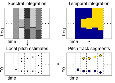
Spectral integration

Local pitch estimates Pitch track segments

Temporal integration

Fig. 8. In anticlockwise sequence, upper-left panel: Regions with different shades of grey represent different spectral groups in each frame. Lower-left panel: dots are

local pitch estimates for the spectral groups. Lower-right panel: two pitch track

seg-ments are produced by linking the local pitch estimates. Upper-right panel: two

spec-tro-temporal fragments are formed corresponding to the two pitch track segments.

5 _{The pitch analysis is based on the autocorrelation method in the ‘Praat’ program}

4.1.2 Temporal integration

Spectral groups produced in the spectral integration stage are combined across

time if their pitch estimates are linked together in the same pitch track

seg-ment, producing spectro-temporal fragments. Each fragment corresponds to

one pitch track segment. This process is illustrated in Fig. 8. The upper-left

panel shows integrated spectral groups for five frames. Regions with

differ-ent shades of grey represdiffer-ent differdiffer-ent spectral groups in each frame. Pitch

estimates for each group in each frame are shown in the lower-left panel. The

lower-right panel shows two smooth pitch track segments that are formed. The

two corresponding spectro-temporal fragments are shown in the upper-right

panel.

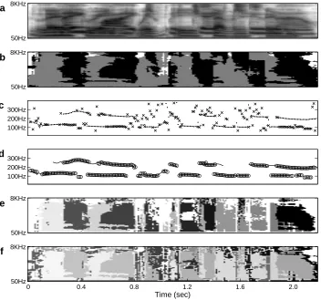
Fig. 10 panel (E) shows the fragments produced corresponding to the pitch

tracks (Fig. 10 panel (D)) in the example of the female(target)/male(masker)

speech mixture. Each fragment is represented using a different shade of grey. It

demonstrates a close match between the generated fragments and the ‘oracle’

segmentation (panel (B)).

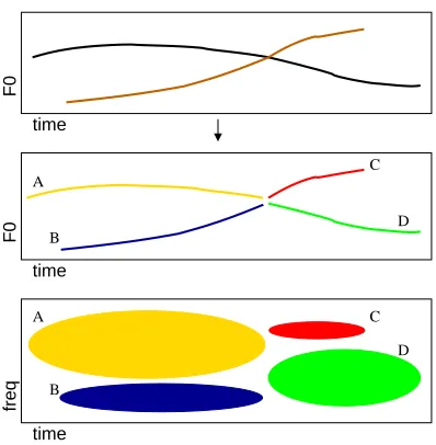
This temporal integration step also has the potential to deal with ambiguous

pitch tracks caused by a similar pitch range from different sound sources.

Consider the situation where two pitch tracks intersect, as illustrated at the

top panel in Fig. 9. The ambiguous pitch tracks will be represented as four

pitch track segments by the system and hence four corresponding

spectro-temporal fragments can be formed (the middle and bottom panel in Fig. 9).

This allows the decision on combining fragments (e.g. {AD, BC} or {AC,

D A

D A

B

B

C

C

freq

F0

F0

time time time

Fig. 9. Top panel: two intersecting pitch tracks. Middle panel: the ambiguous pitch tracks can be represented as four pitch track segments. Bottom panel: four

cor-responding spectro-temporal fragments can be formed allowing a later decision on

fragment combination (e.g. {AD, BC} or {AC, BD}) during the recognition

pro-cess.

4.2 Adding inharmonic fragments

Unvoiced speech lacks periodicity and thus does not produce dendritic

struc-tures in the correlogram domain. The proposed technique which exploits the

periodicity cue skips unvoiced regions and as a result spectro-temporal pixels

corresponding to these regions are missing (e.g. the white region at about 1.1

second in Fig. 10 (e)). The unvoiced regions of the speech signal are

impor-tant in distinguishing words which differ only with respect to their unvoiced

consonants (e.g. /pi:/ and /ti:/). Therefore it is necessary to include some

mechanism that can form coherent fragments for these unvoiced regions.

Hu (2006) gives a systematic study of unvoiced speech segregation. In the

current work, as the focus is on separation of periodic sounds, we employ a

a

50Hz 8KHz

b

50Hz 8KHz

100Hz 200Hz 300Hz

c

100Hz 200Hz 300Hz

d

e

50Hz 8KHz

Time (sec)

f

0 0.4 0.8 1.2 1.6 2.0

50Hz 8KHz

Fig. 10. (a) A ‘ratemap’ representation of the mixture of ‘lay white with j 2 now’ (target, female) plus ‘lay green with e 7 soon’ (masker, male) TMR = 0dB. (b) The

‘oracle’ segmentation. Dark grey: pixels where the value in the mixture is close to

that in the female speech; light grey: the mixture value is close to that in the male

speech; white: low energy regions. (c) Pitch estimates for each source segmentation.

Dots represent the pitch of the stronger source in each frame and crosses

repre-sent the weaker source at that frame. (d) Circles are pitch tracks produced by the

multipitch tracking algorithm; solid lines are the ground-truth pitch tracks. (e)

Frag-ments after temporal integration based on the smooth pitch tracks. (f ) Combining

inharmonic fragments.

(2005). Harmonic regions are first identified in the ‘ratemap’ representation

of the mixture using the techniques described in Section 4.1. The ‘ratemap’

pro-cessed by the ‘watershed algorithm’ (Gonzales et al., 2004). The watershed

algorithm is a standard region-based image segmentation approach. Imagine

the process of falling rain flooding a bounded landscape. The landscape will

fill up with water starting at local minima, forming several water domains.

As the water level rises, water from different domains meets along boundaries

(‘watersheds’). As a result the landscape is divided into regions separated

by these watersheds. The technique can be applied to segregate inharmonic

sources under the assumption that inharmonic sources generally concentrate

their energy in local spectro-temporal regions, and that these concentrations

of energy form resolvable maxima in the spectro-temporal domain. The

inhar-monic fragments produced using this technique are pooled together with the

harmonic fragment as illustrated, for example, in Fig. 10 (F).

5 Fragment-driven Speech Recognition

Given the set of source fragments produced by the processes described in

Section 4, speech recognition can be performed using the Speech Fragment

Decoding (SFD) technique. In brief, the technique works by considering all

possible fragment labellings and all possible word sequences. Each fragment

may be variously labelled as either being a fragment of the target (foreground)

or of the masker (background). A hypothesised set of fragment labels defines

a unique target/masker segmentation that can be represented by a ‘missing

data mask’, mtf – a spectro-temporal map of binary values indicating which

spectro-temporal elements are considered to be dominated by the target, and

which are considered to be masked by the competing sources. Given such a

evaluate the likelihood of each hypothesised word sequence. A Viterbi-like

algorithm is then used to find the most likely combination of labelling and

word-sequence. A full account of SFD theory is provided in Barker et al.

(2005), and for a detailed description of the application of the technique to

simultaneous speech see Coy and Barker (2007).

One weakness of the SFD technique, in the form described above, is that

it produces ‘hard’ segmentations, i.e. segmentation in which each

spectro-temporal element is marked categorically as either foreground or background.

If the early processing has incorrectly grouped elements of the foreground and

background into a single fragment, then there will be incorrect assignments

in the missing data mask that cannot be recovered in later processing. These

problems can be mitigated by using missing data techniques that use ‘soft

masks’ containing a value between 0 and 1 to express a degree of belief that the

element is either foreground or background (Barker et al., 2000). Such masks

can be used in the SFD framework by introducing a spectro-temporal map

to express the confidence that the spectro-temporal element belongs to the

fragment to which it has been assigned. This confidence map, ctf, uses value

in the range 0.5 (low confidence) to 1.0 (high confidence). Given a confidence

map, ctf, each hypothesised fragment labelling can be converted into a soft

missing data mask,mtf, by settingmtf to bectf for time-frequency points that

lie within foreground fragments, and to be 1−ctf for time-frequency points

within missing fragments. A fuller explanation of the soft SFD technique can

be found in Coy and Barker (2007).

In harmonic regions, the confidence map is based on a measure of the similarity

between a local periodicity computed at each spectro-temporal point, and a

fragment as a whole. For each spectro-temporal point the difference between

its periodicity and the global periodicity of the fragment measured at that time

is computed in Hertz, referred to as x. A sigmoid function is then employed

to derive a score between 0.5 and 1:

f(x) = 1

1 + exp(−α(x−β)) (10)

whereα is the sigmoid slope, andβ is the sigmoid centre. Appropriate values

for these parameters were determined via a series of tuning experiments using

a small development data set available in the GRID corpus (see Section 6). It

was found that the values of these parameters are not critical to the overall

performance andα = 0.6 and β =−10 were used in this study.

Confidence scores for the inharmonic fragments in our study are all set to 1.

These confidence scores were used in our coherence evaluation experiment and

also employed (as ‘soft’ masks) along with generated fragments in the SFD

system.

6 Experiments and Discussion

Experiments were performed in the context of the Interspeech 2006 ‘Speech

Separation Challenge’ using simultaneous speech data constructed from the

GRID corpus (Cooke et al., 2006). The GRID corpus consists of utterances

spoken by 34 native English speakers, including 18 male speakers and 16

fe-male speakers. The utterances are short sentences of the form<command:4>

<colour:4> <preposition:4> <letter:25> <number:10> <adverb:4>, as

pairs of end-pointed utterances which have been artificially added at a range

of target-to-masker ratios. All the mixtures are single-channel signals. In the

test set there are 200 pairs in which target and masker are the same speaker;

200 pairs of the same gender (but different speakers); and 200 pairs of

differ-ent genders. The ‘colour’ for the target utterance is always ‘white’, while the

‘colour’ of the masking utterance is never ‘white’. Table 1

Structures of the sentences in the GRID corpus

Verb Colour Prep. Letter Digit Adverb bin blue at a-z 1-9 again lay green by (no ‘w’) and zero now

place red on please

set white with soon

Three sets of coherent fragments were evaluated and compared on the same

task: ‘Fragments - Coy’ are fragments generated by the system reported in Coy

and Barker (2005); ‘Fragments - model’ and ‘Fragments - rule’ are coherent

fragments generated by the proposed system employing the model-based pitch

tracker and the rule-based pitch tracker, respectively.

6.1 Experiment I: Coherence measuring

The fragments are ultimately employed by the speech fragment decoding ASR

system and can be evaluated in terms of the recognition performance achieved.

the quality of fragments is to measure how closely they correspond to the

‘oracle’ segmentation, obtained with the access to the pre-mix clean signals

(see Fig. 10(B) for an example). To do this we derive the ‘coherence’ of a

fragment as follows. If each pixel in a fragment is associated with a weight,

the coherence of the fragment is,

100× max(

P

w1,Pw2) P

w1+Pw2

(11)

wherew1 are a set of weights for pixels in the fragment overlapping one source

and w2 are a set of weights for those which overlap the other source. The

fragments were compared with the ‘oracle’ segmentation to identify the

pix-els overlapping each source. When the decision of each pixel being present or

missing in the fragment is discrete (1 or 0), these weights are all simply ‘1’. In

this study we use the confidence scores described in Section 5 as the weights.

This choice of weight has the desirable effect that incorrect pixel assignments

in regions of low confidence cause less reduction in coherence than incorrect

assignments in regions of high confidence. Note that regardless of the

confi-dence score, some spectro-temporal pixels may be more important for speech

recognition than others. For instance, pixels with high energy representing

vowel regions may be of greater value than low energy pixels. It is less critical

that the latter pixels are correctly assigned, and ideally, the coherence score

should reflect this. In the current measurement, in the absence of a detailed

model of spectro-temporal pixel importance, we make the simple assumption

that each pixel has equal importance.

A histogram with a bin width of 10% coherence (hence 5 bins from

coher-ence 50% to 100%) is computed over the set of fragment cohercoher-ence values.

The fragments are different in size. As smaller fragments are less likely to

overlap different sources, their coherence is inherently higher. For example, at

one extreme, a single-pixel fragment must always have a coherence of 100%.

Although we can get higher coherence scores by generating more small

frag-ments, this would be at the expense of reducing the degree of constraint that

the primitive grouping processes are providing, i.e. a large number of small

fragments produces a much greater set of possible foreground/background

segmentation hypotheses. Furthermore, the increased hypothesis space leads

to an increase in decoding time. This increase can be quite dramatic,

espe-cially if fragments are over-segmented across the frequency axis (see Barker

et al. (2005)). Therefore the aim here is to producelarge and highly-coherent

fragments. With these considerations, in the coherence analysis, we reduce the

effect of the high coherence contributed by small fragments, by weighting each

fragment’s coherence value by its size when computing the histogram, i.e., a

fragment is countedS times if its size isS pixels. The histograms for the three

sets of fragments in all mixture conditions at a TMR of -9 dB are shown and

compared in the top three panels of Fig. 11. They have been normalised by

dividing the count in each bin by the total number of pixels.

The proposed system with either the model-based pitch tracker or the

rule-based pitch tracker produces fragments with very similar quality in terms of

coherence. When compared with the fragments generated by Coy and Barker’s

system, proportionally more fragments with high coherence are produced by

the proposed system. This is probably because pitch estimates of each source

are computed after the sources are separated. The pitch estimates are thus

more reliable and multipitch tracking becomes a much less challenging

50 60 70 80 90 100 0.1

0.2 0.3

Same Talker (ST)

Coherence Bin (%)

Normalised Bin Counts

50 60 70 80 90 100 0.1

0.2 0.3

Same Gender (SG)

Coherence Bin (%)

50 60 70 80 90 100 0.1

0.2 0.3

Different Gender (DG)

Coherence Bin (%)

50 60 70 80 90 100 100

150 200

ST

Coherence Bin (%)

Average Size (# of pixels)

50 60 70 80 90 100 100

150 200

SG

Coherence Bin (%)

50 60 70 80 90 100 100

150 200

DG

Coherence Bin (%)

Fragments − Coy Fragments − model Fragments − rule

Fragments − Coy Fragments − model Fragments − rule

Fig. 11.Coherence measuring results for the three sets of fragments. Top three pan-els: histograms of fragment coherence after normalisation (TMR = -9 dB). Each

fragment’s contribution is weighted by its size when computing the histogram. See

text for details. Bottom three panels: average size of fragments in each corresponding

histogram bin.

the summary of all ACG channels. The multipitch tracker possibly finds more

incorrect tracks through the noisier pitch data. Furthermore, unlike the

pro-posed system where spectral integration is performed before temporal

integra-tion, in Coy and Barker’s system spectral integration relies on the less reliable

pitch tracks. Therefore it is more likely to produce fragments with low

co-herence. Within each system, the best results were achieved in the ‘different

gender’ condition, presumably due to the larger difference in the average F0s

of the sources.

To examine the impact of fragment sizes on the fragment coherence, we also

measured the average size of fragments for each coherence histogram bin,

generated by the proposed system give a very similar pattern. In the coherence

bins higher than 80% their average fragment size is larger than that of Coy

and Barker’s system, although in the low coherence bins it is smaller. This

is, however, acceptable as there are proportionally less fragments with low

coherence in the proposed system.

6.2 Experiment II: Automatic speech recognition

The technique proposed here was also employing within the speech fragment

decoding system reported in Coy and Barker (2007), and using the

experimen-tal set-up developed in Barker et al. (2006) for the Interspeech 2006 Speech

Separation Challenge. The task is to recognise the letter and digit spoken by

the target speaker who says ‘white’. The recognition accuracy of these two

keywords were averaged for each target utterance. The recogniser employed

a grammar representing all allowable target utterances in which the colour

spoken is ‘white’.

In the SFD system a 64-channel log-compressed ‘ratemap’ representation was

employed (see Section 2). The 128-dimensional feature vector consisted of

64-dimension ratemap features plus their delta features. Each word was modelled

using a speaker dependent word-level HMM in a simple left-to-right model

topology, with 7 diagonal-covariance Gaussian mixture components per state.

The number of HMM states for each word was decided based on 2 states per

phoneme. They were trained using 500 utterances from each of the 34 speakers.

The SFD system employs the ‘soft’ speech fragment decoding technique (Coy

The baseline system was a conventional ASR system employing 39-dimensional

MFCC features. A single set of speaker independent HMMs with an

identi-cal model topology employed 32 mixtures per state. They were trained on

standard 13 MFCC features along with their deltas and accelerations.

Following Barker et al. (2006), in all experiments, it is assumed that the target

speaker is one of the speakers encountered in the training set, but two different

configurations were employed: i) ‘known speaker’ - the utterance is decoded

using the set of HMMs corresponding to the target speaker, ii) ‘unknown

speaker’ - the utterance is decoded using HMMs corresponding to each of the

34 speakers and the overall best scoring hypothesis is selected.

We first examine the effect of using soft masks and inharmonic fragments on

the recognition performance. The SFD systems with soft masks and

inhar-monic fragments are then compared to the baseline system and a SFD system

using ‘Fragments - Coy’ with an identical recognition setup.

6.2.1 Effects of soft masks and inharmonic fragments

As discussed in Section 5, an incorrect decision for a spectro-temporal pixel

being present in a fragment cannot be recovered when using discrete masks.

This also affects the decoding process in automatic speech recognition as the

recogniser will try to match speech models with unreliable acoustic evidence.

Therefore we compared the recognition performance using the same set of

fragments with discrete masks and soft masks. The soft masks described in

Section 5 were employed. The discrete masks were produced by simply

re-placing all the pixels in the soft masks with ‘1’ if their values are greater

(Section 4.2) on the recognition performance was also examined. Fig. 12 shows

recognition results of the SFD system using the set of ‘Fragments - rule’ in the

‘known speaker’ configuration. ‘All frags + soft masks’ represents that both

harmonic and inharmonic fragments were used, combined with soft masks. ‘All

frags + discrete masks’ represents results using all fragments but with discrete

masks. ‘Harm frags + soft masks’ is the result with harmonic fragments only

using soft masks.

−9 −6 −3 0 3 6 0 20 40 60 80 100 Overall

Target Masker Ratio (dB)

Percentage Correct (%)

−90 −6 −3 0 3 6 20

40 60 80 100

Same Talker (ST)

Target Masker Ratio (dB)

Percentage Correct (%)

−9 −6 −3 0 3 6 0 20 40 60 80 100

Same Gender (SG)

Target Masker Ratio (dB)

Percentage Correct (%)

−90 −6 −3 0 3 6

20 40 60 80 100

Different Gender (DG)

Target Masker Ratio (dB)

Percentage Correct (%)

All frags + soft masks All frags + discrete masks Harm frags + soft masks

Fig. 12. Recognition accuracy performance of the SFD system using ‘Fragments - rule’ in ‘known speaker’ configuration. ‘All frags + soft masks’: all fragments

(both harmonic and inharmonic fragments) with soft masks, ‘All frags + discrete

masks’: all fragments with discrete masks, and ‘Harm frags + soft masks’: harmonic

fragments only with soft masks.

Results show that the soft masks had a considerable effect on the recognition

discrete masks across all conditions. As shown in the coherence measuring

experiment many fragments have low coherence. Some pixels are unreliable

and by assigning a confidence score to each pixel the speech fragment decoder

is able to weight the pixel’s contribution to the decision. Fig. 12 also shows

that in the ‘same talker’ condition the SFD system using soft masks did not

give any recognition accuracy improvement. One possible reason is that in this

condition, as shown in Fig. 11, there are more fragments with low coherence

and even with soft masks the system could not recover from the errors. Another

reason could be that more ‘important’ pixels were incorrectly assigned in this

condition.

Inharmonic fragments also have some impact on the performance in this

‘let-ter + digit’ recognition task as many let‘let-ters are only distinguished by the

presence/absence of unvoiced consonants, e.g. letter ‘p’, ‘t’ and ‘e’.

6.2.2 Comparison of different fragment sets

All the recognition results in this section were obtained with the ‘soft’ SFD

system using both harmonic and inharmonic fragments. Fig. 13 shows keyword

recognition results of the system using the three sets of coherent fragments

discussed before: ‘Fragments Coy’, ‘Fragments model’ and ‘Fragments

-rule’, in both ‘known speaker’ and ‘unknown speaker’ configurations. The

‘unknown speaker’ results are repeated in Table 2 (model-based pitch tracker)

and Table 3 (rule-based pitch tracker). Note the ‘known - model’ and ‘unknown

- model’ results are essentially the same as those published in Barker et al.

(2006), with minor differences owing to a correction made in the application

−90 −6 −3 0 3 6 20 40 60 80 100 Overall

Target Masker Ratio (dB)

Percentage Correct (%)

−90 −6 −3 0 3 6 20

40 60 80 100

Same Talker (ST)

Target Masker Ratio (dB)

Percentage Correct (%)

−9 −6 −3 0 3 6

0 20 40 60 80 100

Same Gender (SG)

Target Masker Ratio (dB)

Percentage Correct (%)

−90 −6 −3 0 3 6

20 40 60 80 100

Different Gender (DG)

Target Masker Ratio (dB)

Percentage Correct (%)

Known − Coy Known − model Known − rule Unknown − Coy Unknown − model Unknown − rule Baseline

Fig. 13. Keyword recognition results of the proposed system with the

model-based/rule-based pitch tracker compared against the system reported in Coy

and Barker (2005), in both ‘known speaker’ and ‘unknown speaker’ configurations.

The baseline results are taken from Barker et al. (2006).

The SFD systems clearly outperform the baseline across all TMRs and across

all mixture conditions. They are also able to exploit knowledge of the

tar-get speaker identity. The recognition accuracy is significantly higher when

the speaker identity is available. Prior knowledge of the speaker identity only

fails to confer an advantage in the ‘same talker’ condition as one would

ex-pect. Recognition accuracy results using fragments generated by the proposed

system with different pitch trackers are quite similar. This is consistent with

the results in the coherence measuring experiment that with different tracks

the system produced fragments with similar coherence. The results are

Table 2

Keyword recognition correct percentage (%) in unknown speaker configuration using

the model-based pitch tracker.

TMR (dB)

Condition -9 -6 -3 0 3 6

Overall 56.08 57.08 45.92 45.42 69.75 80.42 ST 46.61 44.57 34.62 35.07 55.43 74.43 SG 57.82 62.85 53.63 51.96 76.82 84.08 DG 65.00 65.75 51.50 51.00 79.25 83.75 Table 3

Keyword recognition correct percentage (%) in unknown speaker configuration using

the rule-based pitch tracker.

TMR (dB)

Condition -9 -6 -3 0 3 6

Overall 57.58 57.17 45.17 44.75 69.00 80.67 ST 46.61 45.02 37.10 34.62 54.98 74.43 SG 61.73 63.13 49.16 53.07 77.65 83.52 DG 66.00 65.25 50.50 48.50 76.75 85.00 at low TMRs. The biggest performance gain was achieved in the ‘different

gender’ condition. This occurs because in this condition the two sources are

more likely to have correlated fundamentals, which is difficult to solve purely