Development of a process and toolset to study UCAV flight mechanics using computational fluid dynamics

(1)

Development of a Process and Toolset to Study UCAV

Flight Mechanics using Computational Fluid Dynamics

Thesis submitted in accordance with the requirements of the University of Liverpool for the degree of Doctor in Philosophy

by

David Vallespin

(2)

(3)

Abstract

The work carried out during this project used a Computational Fluid Dynamics code to generate aerodynamic tabular models and aircraft manoeuvre simulations. As an out-come of this work, a validation of the aerodynamic prediction tools and an assessment of tabular models for aircraft flight dynamics applications was made. The Stability and Control Unmanned Combat Air Vehicle has been used as a demonstration case. Valida-tion of computaValida-tional fluid dynamics methods was carried out for highly nonlinear flow topologies using wind tunnel measurements. Integral data, pressure tap measurements and particle image velocimetry information was compared against the predictions over two configurations. Each one had a different leading edge shape distributed along the span of the model. One was sharp throughout with varying leading edge thickness and the other one was mainly rounded. Results showed a good agreement in longitudinal force and moment predictions for low angles of attack. High angles were dominated by a double vortex structure which was very sensitive to incidence angle and leading edge shape. Some wind tunnel effects were noticed in the measurements when predictions were made with and without sting. Overall the numerical predictive capabilities for low and high angles of attack were deemed good for the purpose of flight dynamics model generation.

(4)

(5)

List of Figures

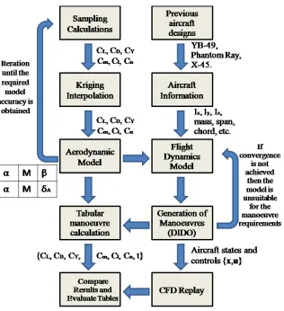
1.1 Flowchart of process described in this thesis. . . 2

2.1 Illustration of the primary and secondary vortices formed over a slender wing [6]. . . 6

2.2 Visualisation of spiral and bubble forms of vortex breakdown [7]. . . 7

2.3 Mean axial velocity contours in a plane through the vortex core: (a) α= 15◦ , (b)α= 10◦ and (c) α= 5◦ , I. Gursul et al. [5]. . . 8

2.4 Illustration of dual vortex structures. . . 9

2.5 Experimentally obtained surface streamline patterns and pressure coef-ficients for a 50◦ leading edge sweep, delta wing atα= 15◦ [5]. . . 10

2.6 Surface oil visualisation of the flow over a sharp edged, 50◦ leading edge sweep, delta wing atα= 0◦ −25◦ [9]. . . 11

2.7 Experimental flow visualisations of two different lambda wings atRe= 2·106 [11]. . . 12

2.8 Illustration of the windward (a) and leeward (b) surface bevelling [14]. . 13

2.9 Experimental values for two lambda configurations of Λ = 40◦ (Model 3) and Λ = 60◦ (Model 4), [11]. . . 14

2.10 Variation of lift coefficient with angle of attack for various leading edge shapes and thicknesses, Gursul [5]. . . 15

2.11 Flowchart of process described in this thesis. . . 19

3.1 Grid point displacements along a block edge [55]. . . 29

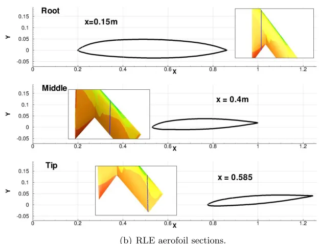
4.1 SACCON geometrical description. . . 34

4.2 RLE model leading edge grit and gap filling. . . 35

4.3 Pressure port and kulite arrangement on the SACCON wind tunnel model [63]. . . 36

4.4 SACCON PIV measurements. . . 37

4.5 SACCON model setup in the wind tunnel. . . 38

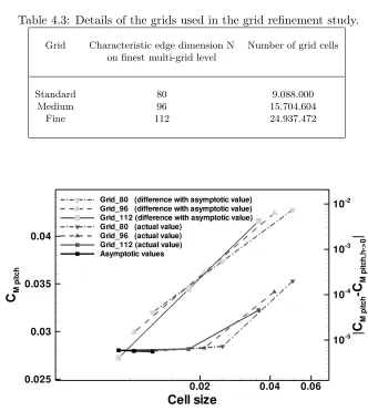
4.6 Results of the grid convergence study for the SACCON configuration. . 39

4.7 SACCON model grid topologies for PMB calculations. . . 41

(8)

4.9 Boundary layer velocity profile at point (0.3m,0.15m) over the top

sur-face of the wing for the RLE and SLE models. . . 42

4.10 PMB k-ω flow solutions for the SACCON UCAV at α= 17◦ and Re= 1.93·106_{. . . .} ₄₃

4.11 Integral data from experimental results and PMB computations for the round leading edge model. . . 44

4.12 Difference in CP distribution between PMB and ENSOLV solutions. . . 45

4.13 PMB predictions of pressure coefficient distribution (baseline k-ω) with plots of experimental measurements and computed results for the SLE model. . . 47

4.14 Liverpool’s predicted flow topology (baseline k-ω) for the SLE. . . 49

4.15 PMB predictions (baseline k-ω) of downstream velocity, U, across the vortex core. . . 50

4.16 PMB predictions of pressure coefficient distribution (baseline k-ω) with plots of experimental measurements and computed results for the RLE model. . . 52

4.17 Liverpool’s predicted flow topology (Baseline k-ω) for the RLE. . . 55

4.18 CFD data comparison with PIV measurements for the RLE model at α= 16◦ . . . 55

4.19 CFD data comparison with PIV measurements for the RLE model at α= 18◦ . . . 56

4.20 Integral data from experimental results and PMB computations for the sharp leading edge model. . . 58

4.21 Distributions of change in moment over the top and bottom SACCON RLE surfaces. . . 60

4.22 Pitch forced motion integral data from experiments and PMB computa-tions for the sharp leading edge model at α0 = 10◦ and an amplitude of 5◦ . . . 62

4.23 Pitch forced motion integral data from experiments and PMB computa-tions for the round leading edge model atα0 = 10◦ and an amplitude of 5◦ . . . 63

5.1 Flowchart describing the flight dynamics assessment methodology. . . . 68

5.2 Influence of centre of gravity location on the pitching moment coefficient. 70 5.3 Thrust vectoring technique schematics. . . 71

5.4 Control surface grid illustrations. . . 71

5.5 Aileron control surface aerodynamic characteristics. . . 72

5.6 Image of the YB-49 Aircraft [77]. . . 73

5.7 α withβ and M achsweeps for the lift coefficient. . . 77

(9)

5.9 α withβ and M achsweeps for the side force coefficient. . . 79

5.10 α withβ and M achsweeps for the pitching moment coefficient. . . 81

5.11 Cp distribution at different sideslip angles. . . 82

5.12 α withβ and M achsweeps for the rolling moment coefficient. . . 83

5.13 α withβ and M achsweeps for the yawing moment coefficient. . . 84

5.14 Aileron effectiveness for the range of αwithβ andM achsweeps for the rolling moment coefficient. . . 85

5.15 Aileron effectiveness for the range of αwithβ andM achsweeps for the yawing moment coefficient. . . 86

5.16 Effect of aileron on aircraft forces and pitching moment coefficients for the range ofα and M ach. . . 87

5.17 Time-accurate CFD predictions of the longitudinal force and moment coefficients. . . 88

5.18 Minimum and maximum rotation rate points in the CL and Cm loops. . 89

5.19 Dynamic derivative predictions using two different methods. . . 89

5.20 Normal force coefficient predictions using a linear regression model com-pared to the time-accurate CFD predictions. . . 90

5.21 Pitching moment coefficient predictions using a linear regression model compared to the time-accurate CFD predictions. . . 91

5.22 Motion variables notation. . . 93

6.1 SACCON manoeuvre trajectories. . . 98

6.2 Implemented SACCON model trim states. . . 99

6.3 SACCON pull-up trajectory. . . 101

6.4 SACCON motion during a slow pull-up. . . 102

6.5 SACCON forces and moments during a slow pull-up. . . 104

6.6 SACCON slow lazy eight trajectory. . . 105

6.7 SACCON motion during an Immelmann turn. . . 106

6.8 SACCON forces and moments during a slow Immelman turn. . . 107

6.9 SACCON longitudinal forces and moments during a slow Immelman turn against angle of attack. . . 108

6.10 SACCON 90◦ turn trajectory. . . 109

6.11 SACCON motion during a 90◦ turn. . . 110

6.12 SACCON forces and moments during a 90◦ turn. . . 111

6.13 Transient flow effect on discrepancies during a 90◦ turn. . . 113

6.14 Cp and ∆Cp distributions at 6 seconds during the 90◦ turn. . . 113

6.15 SACCON longitudinal forces and moments during a 90◦ turn against angle of attack. . . 114

6.16 SACCON lazy eight trajectory. . . 115

(10)

6.18 SACCON forces and moments during a slow lazy eight. . . 118 6.19 Cp and ∆Cp distributions at different times during the slow lazy eight. . 119

6.20 ∆Cp distributions over two periods during the slow lazy eight manoeuvre.120

6.21 SACCON longitudinal forces and moments during a slow lazy eight against angle of attack. . . 121 6.22 SACCON forces and moments during a fast lazy eight. . . 123 6.23 Cp and ∆Cp distributions at different times during the fast lazy eight. . 124

6.24 SACCON longitudinal forces and moments during a fast lazy eight against angle of attack. . . 124

(11)

Acknowledgement

I would like to extend my gratitude to my supervisors, Professor Ken Badcock and Professor George Barakos, and all the members of the CFD Lab, past and present, without whom this work would have not been possible.

I would like to thank Dr. Malcolm Arthur, Professor Russ Cummings and Okko Boelens for their encouraging support as well as the members of the NATO RTO AVT-161 techical group for their feedback throughout the duration of the project. The effort from the members that took part in the SACCON model design, manufacture and wind tunnel measurements is very much appreciated.

I am grateful for the financial support given by the Engineering and Physical Sci-ences Research Council (EPSRC) and QinetiQ. Also to the 2nd _{Applied Aerodynamics}

Consortium for providing computing time in the HECToR Supercomputer.

I would like to thank my friends in Liverpool and back home for always providing means of distraction and words of support throughout the years.

(12)

(13)

Publications

Conference Papers

Vallespin D, Boelens O, Da Ronch and Badcock KJ. SACCON CFD Simulations Us-ing Structured Grid Approaches,Proceedings of the 28th _{AIAA Applied Aerodynamics}

Conference, AIAA-2010-4560, June 2010.

Vallespin D and Badcock KJ. Assessment of the Limits of Tabular Aerodynamic Models for Flight Dynamics Analysis using the SACCON UCAV Configuration. Pro-ceedings of the RAeS Aerodynamics Conference 2010. Applied Aerodynamics: Capabil-ities and Future Requirements, July 2010.

Journal Papers

Vallespin D, Da Ronch A, Badcock K and Boelens O. Vortical Flow Prediction Valida-tion for an Unmanned Combar Air Vehicle Model. Journal of Aircraft, 48(6):1948-1959, 2011. doi: 10.2514/1.56673.

Vallespin D, Badcock KJ, Da Ronch A, White MD, Perfect P and Ghoreyshi M. Computational Fluid Dynamics Framework for Aerodynamic Model Assessment,

Progress in Aerospace Sciences, 52:2-18, 2012.

Vallespin D, Boelens O and Badcock KJ. SACCON CFD Simulations Using Struc-tured Grid Approaches. NATO RTO AVT-161 Final Report, Chapter 11, 2011.

Vallespin D, Cummings RM and Boelens O. Comparison of results for predicting highly non-linear vortical flow features of the UCAV SACCON configuration. NATO RTO AVT-161 Final Report, Chapter 19, 2011.

Da Ronch A, Vallespin D, Ghoreyshi M and Badcock KJ. Evaluation of Dynamic Derivatives Using Computational Fluid Dynamics,Accepted in the AIAA Journal, 2011.

(14)

(15)

Nomenclature

Variables

A Amplitude of angle of attack [◦

]

CD Coefficient of drag, CD = 2(_ρ∞DragV∞2S) CL Coefficient of lift, CL= _ρ2(∞Lif tV∞2S) CMq Coefficient of pitching moment due to pitch rate

CMα˙ Coefficient of pitching moment due to rate of change of angle of attack

CN Coefficient of normal force

CY Coefficient of side force

CZq Coefficient of normal force due to pitch rate

CZα˙ Coefficient of normal force due to rate of change in angle of attack

Cj Coefficient of force or moment

Cjq Coefficient of force or moment due to pitch rate

Cjα˙ Coefficient of force or moment due to pitch rate

¯

Cj Combined pitching dynamic derivative

¯

Cjα In-phase component of force or moment coefficient ¯

Cjq Out-of-phase component of force or moment coefficient

Cl Coefficient of rolling moment Cl= 2(Rolling M oment_ρ )

∞V

2

∞Sbref Cm Coefficient of pitching moment, Cm= 2(P itching M oment_ρ )

∞V

2

∞Scref Cn Coefficient of yawing moment Cn= 2(Y awing M oment_ρ )

∞V

2

∞Sbref Cp Coefficient of pressure, CL= _ρ2(∞Lif tV∞2S) CpSS Coefficient of pressure from steady state solution

CpR Coefficient of pressure from unsteady replay solution

Cp_ti Coefficient of pressure from solution at time ti

CX_adynamic Coefficient of dynamic aerodynamic contribution

CX_astatic Coefficient of static aerodynamic contribution

CX_δail Coefficient of aileron aerodynamic contribution

E Total energy

F Running cost

Fi Inviscid flux vector along the x-axis

ˆ

(16)

Fv Viscous flux vector along the x-axis

ˆ

Fv

Viscous flux vector along the x-axis in curvilinear form

Gi Inviscid flux vector along the y-axis

ˆ

Gi Inviscid flux vector along the y-axis in curvilinear form

Gv Viscous flux vector along the y-axis

ˆ

Gv Viscous flux vector along the x-axis in curvilinear form

H Total enthalpy

Hi Inviscid flux vector along the z-axis

ˆ

Hi Inviscid flux vector along the z-axis in curvilinear form

Hv Viscous flux vector along the z-axis

ˆ

Hv Viscous flux vector along the z-axis in curvilinear form

IX Moment of inertia about x-axis [kg−m2]

IY Moment of inertia about y-axis [kg−m2]

IZ Moment of inertia about z-axis [kg−m2]

J Jacobian determinant

L Characteristic length [m]

L Lift force [N]

ˆ

L Rolling moment [N m]

ˆ

M Pitching moment [N m]

M Mach number, M = V∞

a

ˆ

N Yawing moment [N m]

Pk Turbulence kinetic energy production term

Pr Prandtl number

Prt Turbulent Prandtl number

Pω Specific dissipation rate production term

R(W_i,j,k) Flux residuals

Re Reynolds number, Re= ρ∞V∞c_ref

µ

S Reference surface area [m2]

Sref Reference surface area [m2]

T Temperature [K]

T0 Reference temperature [T0 = 288.16K]

U Velocity along the x-axis in body frame of reference [m/s]

U∞ Freestream velocity [m/s]

V Velocity along the y-axis in body frame of reference [m/s]

V∞ Freestream velocity [m/s]

V Velocity vector [m/s]

Vi,j,k Cell volume

W Column matrix of conserved variables

ˆ

(17)

Wi,j,k Flux variables

W Velocity along the z-axis in body frame of reference [m/s]

Wa Aircraft weight [N]

X Force along the x-axis [N]

a Speed of sound [m/s]

bref Reference span [m]

cref Reference chord length [m]

croot Root chord length [m]

d Moment arm length [m]

e Specific internal energy

f Frequency of oscillation [Hz]

fi Body forces

k Non-dimensional frequency ˆ

k Thermal conductivity

k′

Turbulence kinetic energy per unit mass

lthrust Distance from thrust force to CG [m]

p Pressure [N/m2]

pi Instantaneous pressure [N/m2]

¯

pi Mean pressure component [N/m2]

p′

i Turbulent fluctuating pressure component [N/m2]

ˆ

p Roll rate [◦

/s] ˙ˆ

p First derivative of roll rate [◦ /s2] ˙

q Rate of volumetric heat addition per unit mass ¯

q Dynamic pressure [N/m2_]

ˆ

q Pitch rate [◦

/s] ˙ˆ

q First derivative of pitch rate [◦ /s2_]

ˆ

r Yaw Rate [◦

/s] ˙ˆ

r First derivative of yaw rate [◦ /s2]

t Time [s]

t0 Initial time [s] tf Final time [s]

ˆ

t Non-dimensional time

u(·) Control vector

u Velocity component along the x-axis

ui Instantaneous velocity component along the x-axis

¯

ui Mean velocity component along the x-axis

u′

i Turbulent fluctuating velocity component along the x-axis

v Velocity component along the y-axis

(18)

¯

vi Mean velocity component along the y-axis

v′

i Turbulent fluctuating velocity component along the y-axis

w Velocity component along the z-axis

wi Instantaneous velocity component along the z-axis

¯

wi Mean velocity component along the z-axis

w′

i Turbulent fluctuating velocity component along the z-axis

x x-coordinate [m]

xj Coordinate axis, where xj =x,y orz [m]

x(·) State vector

y y-coordinate [m]

y+ _{Non-dimensional distance of first cell from wall}

z z-coordinate [m]

∆ Change in

∆CL1 Change in CL due to data fusion errors

∆CL2 Difference in CL between steady and unsteady simulation

∆CL3 Change in CL due to vortex transient effects

∆Cm1 Change in Cm due to data fusion errors

∆Cm2 Difference in Cm between steady and unsteady simulation

∆Cm3 Change in Cm due to vortex transient effects

Λ Sweep angle [◦

]

α Angle of attack [◦

]

αtrim Angle of attack at trim [◦]

ˆ

α Closure coefficient

˙

α First derivative of angle of attack

β Angle of sideslip [◦

]

βtrim Angle of sideslip at trim [◦]

ˆ

β, ˆβ∗

Closure coefficients

γ Flight path angle [◦

] ˆ

γ Ratio of specific heats [ˆγ = 1.4]

δele Elevator deflection angle [◦]

δail Aileron deflection angle [◦]

δrud Rudder deflection angle [◦]

ζ Local coordinate axis in curvilinear form

η Local coordinate axis in curvilinear form

ηT Throttle [%]

ηθ Pitch thrust vector angle [◦]

ηψ Yaw thrust vector angle [◦]

θ Angle of pitch [◦

]

(19)

µ0 Reference laminar viscosity [µ0 = 1.7894·10−5kg/ms] µt Turbulent eddy viscosity [kg/ms]

ξ Local coordinate axis in curvilinear form

ρ Density of air [kg/m3_]

ρi Instantaneous density [kg/m3]

¯

ρi Mean density component [kg/m3]

ρ′

i Turbulent fluctuating density component [kg/m3]

ˆ

σ, ˆσ∗

Closure coefficients

τ Pseudo time-step

τij Viscous stress tensor

φ Angle of roll [◦

]

ψ Angle of yaw [◦

]

ω Frequency of oscillation [rad/s]

ωx Vorticity in the y-z plane

ωy Vorticity in the x-z plane

ωz Vorticity in the x-y plane

ω′

Specific dissipation rate

∞ Freestream condition

Abbreviations and Acronyms

AVT Applied Vehicle Technology CFD Computational Fluid Dynamics

CG Centre of gravity

DNW German-Dutch Wind Tunnels DPT Dynamic Pressure Transducer DLR German Aerospace Center

DoF Degrees of Freedom

DNW-NWB German-Dutch Wind Tunnels

EADS MAS European Aeronautic Defence and Space Company ENFLOW NLR Navier-Stokes flow simulation system

ENSOLV NLR Navier-Stokes flow solver

EPSRC Engineering and Physical Sciences Research Council F&M Forces and moments

IDVD Inverse Dynamics Calculation in the Virtual Domain ISS International Space Station

(20)

MUSCL Monotone Upstream-centred Schemes for Conservation Laws NATO North Atlantic Treaty Organisation

NASA National Aeronautics and Space Administration NLP Non-Linear Programming

ONERA The French Aerospace Lab PIV Particle Image Velocimetry PMB Parallel Multiblock

PMP Pontryagin Maximum Principle

PS Pseudospectral Methods

RANS Reynolds Averaged Navier-Stokes

RLE Round Leading Edge

RTO Research and Technology Organisation SACCON Stability And Control Configuration

SLE Sharp Leading Edge

TVD Total Variation Diminishing TNT Turbulent Non-turbulent UCAV Unmanned Combat Air Vehicle

(21)

Chapter 1

Introduction

An adequate understanding of the aerodynamics of an aircraft is of utmost impor-tance in aircraft design. Despite this, in a traditional aircraft design process, it is at a relatively late stage that an accurate prediction of the aerodynamic loads becomes available, obtained from wind tunnel experiments or flight tests. Any major changes in the configuration late in the design can dramatically increase costs. For this reason since the 1960’s, simulation methods have been adopted throughout the design stages as fundamental engineering tools [1]. Analytical engineering methods have been heav-ily relied on to provide estimates of aircraft force and moment characteristics. These mainly empirical methods can be insufficient, particularly when a configuration lacks any empirical support. More reliable first principles computational methods have been developed and implemented. The potential to use numerical methods has progressed since the start of the digital era and great strides have been made in the fields of struc-tural analysis, flight simulation and fluid dynamics which have been widely documented in the literature. Numerical aerodynamic prediction tools are commonly referred to as Computational Fluid Dynamics (CFD). The challenge nowadays is to obtain the best performance out of these methods with the minimum amount of effort and cost and in a manner that integrates with other disciplines in the engineering design process.

(22)

and dangerous for the commercial type of aircraft although it is vital for adequate pilot training [3]. Hence, it is clear that there is a demand for high fidelity aerodynamic data throughout the operational flight envelope and beyond. Technological developments such as Fly by Wire (FBW) systems can potentially reduce this type of occurrence, although it is the case that to design and improve these systems a good knowledge of the aerodynamic behaviour throughout the flight envelope is required. It is an important open question as to how much fidelity in aerodynamic prediction is enough for such applications.

In the military sector, a major development in recent years has been the establish-ment of Unmanned Air Vehicles (UAVs) for a wide range of military operations. These span from Surveillance, Reconnaissance and Intelligence (ISR) to “persistent strike” functions [4]. As the technology matures new designs will keep replacing traditional manned aircraft operations. From an engineering point of view, new challenges are present in aircraft design. The removal of human survivability constraints has widened operational envelopes allowing for new design concepts. In turn, this requires an ex-tensive study of the aircraft’s performance from the conceptual stages of the design process. The autonomous nature of these aircraft requires a good understanding of flight dynamics behaviour prior to adequate control law design. Moreover, the blunt leading edge and low angle wing sweep of typical Unmanned Combat Air Vehicles (UCAVs) has not been studied as extensively as traditional highly swept wings. These configurations have been adopted more recently for reasons other than aerodynamics, mainly signature. This type of configuration has proven to be a challenging case for CFD solvers, as will be seen in this study.

Figure 1.1: Flowchart of process described in this thesis.

(23)

(24)

(25)

Chapter 2

Literature Survey

The current understanding of vortical flow behaviour over delta wings is reviewed in Ref. [5] where a distinction is made between slender and non-slender wings, the latter being those with a leading edge sweep angle lower than 65◦

. Non-slender delta wings have recently become an important area of aerodynamic research due to their increasing use for UCAV configurations. Although much of the existing knowledge on vortical flow structures is related to slender delta wings, these flows make a relevant comparison with those of non-slender delta wings. One of the main differences between the two is that two primary vortices occur over the lower leading edge sweep wings at high angles of attack. These two vortices are distinct and have the same sense of rotation whereas a single primary vortex structure is present for the slender wing.

For a slender, sharp edged delta wing boundary layer separation is at the leading edge. As a result of this, a free, three-dimensional shear layer emanates from the wing’s leading edge which initiates a primary vortex, as illustrated in Fig. 2.1. The regions of high vorticity at the core are surrounded and continuously fed by the shear layer. When the primary vortex interacts with the boundary layer on the upper surface of the wing it gives rise to boundary layer separation and the formation of a secondary vortex of the opposite sign of vorticity. A tertiary vortex may take place underneath the secondary one depending on the nature of the boundary layer and the viscosity of the flow. The flow through the symmetry plane of the body remains attached.

(26)

to the high rotation of the flow in the vortex core a region of low local static pressure is produced yielding a suction force on the upper surface called non-linear or vortex lift.

Figure 2.1: Illustration of the primary and secondary vortices formed over a slender wing [6].

(27)

[image:27.612.166.474.71.299.2]

Figure 2.2: Visualisation of spiral and bubble forms of vortex breakdown [7].

large scale turbulent flow downstream.

Gursul et al. [5] describes the post-breakdown region as where the primary vortex core disintegrates into a large number of fine-scale, highly unsteady flow features. Only a large region of vortical flow made up of these small structures can be distinguished. In the case of highly swept wings, the secondary flow also follows the same pattern which is why pockets of opposite sign vorticity can still be seen in this unsteady region. It is also possible to find pockets of reversed axial flow in the breakdown region, as described later, with a large region of fluctuating kinetic energy.

Yaniktepe and Rockwell [8] identified three stages in the low sweep delta wing vortex breakdown process. First, small scale undulations, or spiralling, occur at the vortex core associated with the shear layer instabilities and the onset of breakdown. Secondly, the filament is seen to thicken and become small again at what is defined as the pinch off region, as described by Gursul [5]. Finally, breakdown occurs characterised by an abrupt expansion of the filament where the particles are diffused over a broad area. An increase in pressure accompanies this broken down flow region for which some examples are shown in Section 4.3.2.

An important characteristic describing the vortex stages is the axial flow velocity through the core. For the slender wing case, the axial flow decelerates downstream of the breakdown location, changing from a jet-like to wake-like type of flow. The onset of this is very abrupt and the core can expand by a factor of 3 of its original cross-sectional area. It can be defined as the point of maximum upstream penetration of the reversed axial flow [9]. According to Gursul et al. [5], for his non-slender wing (Λ = 50◦

(28)

angles of attack above 10◦

the vortex core upstream from breakdown has a jet-like flow. After breakdown, the flow slows down and becomes wake-like. At lower angles of attack the jet-like region is no longer present, although the flow in the core upstream from the vortex breakdown has a higher velocity than that downstream from it, as shown in Fig. 2.3. The switching point pinpoints the location of vortex breakdown. Nonetheless, the breakdown of high sweep configurations is more abrupt. The experiments carried out by Ol and Gharib [10] at a Reynolds number of 1.54·104 on a 65◦

swept back wing demonstrate a nearly linear increase in peak vortex core velocity as the angle of attack is increased, which is not the case for a non-slender wing. Their results prove the jet-like and wake-jet-like behaviours of the slender and non-slender configurations with slight discrepancies at the angles of attack at which they occur. These could be attributed to the influence of the Reynolds number. Reducing this number drives the flowfield toward a state of unperturbed freestream. It was shown that as the Reynolds number decreases lower variations and smaller gradients are seen for the axial and azimuthal velocities throughout a given flow structure.

Figure 2.3: Mean axial velocity contours in a plane through the vortex core: (a)α= 15◦

, (b)α= 10◦

and (c) α= 5◦

, I. Gursul et al. [5].

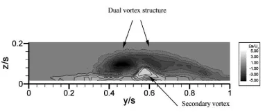
Taylor et al. [9] concluded from an experimental study with a 50◦

sweep delta wing at a freestream Reynolds number around 3·104 that an elongated region of separated flow transforms into a dual vortex structure. This occurs further downstream from the formation of the primary vortex. Here, as the secondary flow separates from the body surface, it impinges on the separated shear layer emanating from the leading edge splitting it into two vortices of the same sign, as shown in Fig. 2.4 (a). This gives rise to the second primary vortex which is slightly weaker and smaller than the first vortex. Experiments carried out on a sharp 2% thick delta wing with a sweep of 50◦

(29)

Reynolds numbers of 104 _{[9] demonstrated that dual vortical flows may occur at angles}

of attack as low as 5◦

. As the incidence was further increased to 15◦

the clear dual vortex structure disappeared to form a structure that resembles those of highly swept wings, with primary, secondary and tertiary vortices. Therefore, it can be said that the splitting of the primary vortex into two by the boundary layer vorticity disappears as the angle of attack is increased. Ol and Gharib [10] performed a similar experiment and came to the same conclusion. Their results can be seen in Figure 2.4 (b).

(a) Computed illustration of a dual vortex struc-ture over a 50◦

leading edge sweep, delta wing at α= 5◦

[5].

(b) Crossflow vorticity field at a section across the vortices for a 50◦

leading edge sweep, delta wing atα= 7.5◦

[image:29.612.120.310.200.320.2]

[9]

[image:29.612.330.521.245.326.2]

Figure 2.4: Illustration of dual vortex structures.

Figure 2.5 shows an experimentally obtained streamline pattern for the sharp edged, 50◦

sweep delta wing at 15◦

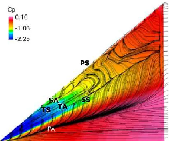
angle of attack [5]. The positions of the primary, secondary and tertiary attachment and separation lines can be seen for that case as PA, SA, TA and PS, SS, TS, respectively. This shows that secondary and tertiary vortices can occur over non-slender configurations, as shown in Section 4.3.2 in this thesis.

With increasing incidence, the attachment boundary moves inboard towards the wing’s centre line until this line is no longer visible, corresponding to wing stall. It is interesting to follow the development of these regions as the angle of attack is varied from 0◦

to 25◦

, illustrated by Taylor et al. [9] in Figure 2.6. For the case of an angle of attack as low as α = 2.5◦

, coherent leading edge vortices can be seen. These are recognised by the spanwise dyed flow patterns ranging from the primary attachment to the secondary separation lines.

Whenα= 10◦

is reached, the initial primary vortex becomes much more prominent than the second and gets shifted away from the surface and inboard on the wing. The flow patterns at α= 15◦

show a primary reattachment line downstream from the apex which then soon fades away, meaning that the vortex has broken down with its consequent expansion. At α = 21.25◦

(30)

[image:30.612.173.469.77.323.2]

Figure 2.5: Experimentally obtained surface streamline patterns and pressure coeffi-cients for a 50◦

leading edge sweep, delta wing atα = 15◦

[5].

upstream and stalled flow covers the wing surface. This evolution of the vortex structure as the angle of attack increases demonstrates the increasing similarity with the structure seen for slender bodies in terms of growth of the main vortex structure and upstream movement of the breakdown location with increasing angle of attack.

A direct comparison was made by Woods [11] between a slender (60◦

sweep) and a non-slender (40◦

sweep) lambda wing using wind tunnel experiments at a Reynolds number of 2·106_{. His results agree with the vortex behaviour seen by Gursul et al.}

[12], Taylor et al. [9] and Ol and Gharib [10] which suggests a similarity between delta and lambda wing flow behaviour, shown in Figure 2.7. Over the non-slender wing a dual vortex structure was present atα= 10◦

. The second primary vortex was seen to reduce in size as the first primary vortex became dominant atα= 15◦

and an enlarged single primary vortex was present at α = 20◦

with reversed flow occurring over most of the top surface. The highly swept wing images show the path of the primary vortex atα= 10◦

and 15◦

where it is clear that the core does not move inboard as rapidly as the lower swept case.

(31)

[image:31.612.152.501.185.574.2]

Figure 2.6: Surface oil visualisation of the flow over a sharp edged, 50◦

leading edge sweep, delta wing atα= 0◦

−25◦

(32)

(a) Λ = 40◦

atα= 10◦

(b) Λ = 40◦

atα= 15◦

(c) Λ = 60◦

atα= 10◦

(d) Λ = 60◦

[image:32.612.115.527.193.576.2]

atα= 15◦

(33)

noticed by Gad-el-Hak and Blackwelder [13] that this vortex sheet rolls up periodically into these vortical substructures. Another effect of this flow instability leads to vortex wandering around the mean core location in the y-z plane. This leads to the vortex core moving in an oval pattern in the same sense of rotation as the vortex swirl.

It is seen that for non-slender wings the post-breakdown behaviour is similar to that of slender wings, in the sense that a spiral mode can be recognised as shown by Gursul et al. [5] although not as abrupt. It is relevant to notice that the instabilities do not necessarily occur symmetrically over full wing configurations experimentally or in computations. The variation of streamwise vortex breakdown location on each side of the configuration can affect the lateral characteristics of the aircraft. The resulting asymmetric load distribution can yield significant lateral activity. The frequency of the breakdown oscillation and the magnitude of the resulting loads will determine how much impact these have on the overall performance. For slender wings, fluctuations of up to 10% of the chord length have been observed [5], whereas for non-slender wings, up to 50% variation along the chord has been registered [10]. Taylor et al. [9] showed that the vortices disintegrate and reform on a quasi-alternating basis in the range of 12.5◦

−17.5◦

where oscillating motions reached an amplitude of 40% of the chord. Experiments carried out by Miau et al. [14] on a 50◦

sweep delta wing at a free stream Reynolds number of 7·103 investigated the role of the leading edge shape in the overall flow behaviour. They looked at the flow over several different types of sharp, round and blunt leading edges and noticed differences in the streamlines and the vortex paths. More specifically, the shapes with bevelling on the windward surface had a leading edge vortex at 10◦

[image:33.612.264.374.558.669.2]

angle of attack whereas those with blunt shape or bevelling on the leeward surface did not. Figure 2.8 shows a schematic of the two types of sharp leading edge shape and the flow around it. Also, the rounded geometry developed a leading edge vortex further downstream than the sharp one, at 20% of the chord. It was concluded that the initial trajectory of the separated shear layer is what determines the overall vortex behaviour on the upper surface.

Figure 2.8: Illustration of the windward (a) and leeward (b) surface bevelling [14].

(34)

Reynolds numbers. Gordnier et al. [15] carried out a study on a 50◦

sweep delta wing looking at the influence of the Reynolds number on the resulting vortical flow. Their computations and experiments focused on the unsteady behaviour of the flow at three Reynolds numbers: 2 x 105_{, 6.2 x 10}5 _{and 2 x 10}6_{. They concluded that the}

vortex breakdown location moved upstream and then downstream again with helical substructures becoming more numerous in the shear layer and developing further up-stream as the Reynolds number increased. It is important to mention that studies with varying leading edge geometry are rare.

According to Gursul et al. [5] non-slender delta wings have lower maximum lift coefficients and steeper lift curve slopes than slender delta wings, which agrees with experimental results shown in Fig. 2.9. This could be caused by a lower lift contribution from vortex suction over the the non-slender wing since these produce weaker vortices and, therefore, lower suction peaks. The fact that the primary vortex breakdown travels upstream over the low sweep wing at a faster rate causes the early stall and subsequently a lower maximum lift coefficient. The drag coefficient patterns show a better behaviour for the non-slender wing which reaches a lower value at stall than the slender wing.

(a)CLvsα (b) CD vsα Figure 2.9: Experimental values for two lambda configurations of Λ = 40◦

(Model 3) and Λ = 60◦

(Model 4), [11].

(35)

[image:35.612.131.504.106.367.2]

in stall angle due to this geometric factor, as shown in Figure 2.10.

Figure 2.10: Variation of lift coefficient with angle of attack for various leading edge shapes and thicknesses, Gursul [5].

So far in this section we have seen that the leading edge sweep angle and profile distribution are two important characteristics determining the flow topology around delta wings. The literature has shown that weaker vortices occur as the sweep angle of a wing is reduced, although their influence on the overall aerodynamic loads is still predominant at high angles of attack. Non-slender wings show an interesting non-linear behaviour in the early post-stall region. It can arise as a dual vortex structure or as unsteady vortex wandering or vortex breakdown motion.

Understanding the aerodynamics of aircraft in motion has been the purpose of various wind tunnel campaigns since the late 1970s. Since that time, a wide range of test rigs has been designed to recreate simple oscillatory motions [16]. More recently, Rein et al. [17] modelled complex manoeuvres using novel rig designs for fighter configurations such as the X-31. Many details were included in the model geometry including moving control surfaces and motions based on previous flight tests. Issues such as Reynolds number similarities, ground effects and fluid-motion coupling are present, as described by Ericsson and Beyers [18].

(36)

shock wave formation can be predicted with confidence in the results. A recent study by Knight et al. [19] assessed the capabilities of a range of CFD codes to accurately predict shock wave formation over conical and cylindrical test cases. Results were com-pared with experimental measurements with good agreement overall with the exception of a low enthalpy, high Reynolds number test case in which the numerical methods dis-agreed. The use of CFD methods for flow separation and vortical flow prediction for a range of Reynolds and Mach numbers has been discussed previously in this chapter and good agreement has been seen with wind tunnel measurements. The CFD code used in this study, Parallel Multiblock (PMB), has been validated over the last twenty years for a wide range of flows. A detailed description of the numerical method is given in Chapter 3. Schiavetta et al. [20] investigated the effects of shock wave interaction with vortex breakdown for a slender delta wing configuration. The predictions from PMB were validated against wind tunnel measurements and other numerical methods with good agreement between the sources. The small scale turbulent structures occurring inside and donwstream from a UCAV weapons bay was investigated using PMB by Lawson et al. [21].

State of the art CFD simulations can be used for early detection of unwanted effects regarding structural integrity, noise or stability and control behaviour, amongst others. Extensive validation work has been carried out using PMB for a range of cases from fixed wing to rotorcraft aerodynamic simulations coupled with aeroelastic models [22, 23]. Marques et al. [24] studied the effects of ice over wing aerofoils and evaluated the detrimental effect of such occurence on the aerodynamic performance.

In an attempt to extend the use of computational methods, considerable effort has focused on predicting flight dynamics performance of aircraft based on a range of aerodynamic and flight dynamic models. Kruger [25] described a method which coupled linear aerodynamic strip theory with the equations of motion and a structural model based on a Multi Body System (MBS). Control over the motion was achieved by introducing changes to the local lift forces at the sections where the control surfaces were located. Important differences were noted between simulated pull-up manoeuvres for rigid and flexible aircraft. A more complex aerodynamic model was used by Costello and Sahu [26] in their study of projectile flight trajectories. Their aim was to validate a rigid body simulation of a projectile with spark range testing results. A full Reynolds Averaged Navier-Stokes (RANS) method was used in a time-accurate manner. The forces and moments computed by the CFD are transferred to the six degrees of freedom (DoF) equations of motion. Results show the free response behaviour of the projectile to control inputs.

(37)

free path from the start to finish is found. Using agility metrics, the manoeuvre is split into a sequence of elemental maneouvres in time, such as level flight, climb, descent, roll, etc. Finally, a feasibility study is made to determine whether it is dynamically possible for the aircraft to achieve the manoeuvre. The dynamics feasibility is assessed using the state boundaries of a flight envelope and maximum and minimum values for structural loads and control surface actuator saturation.

A recent study by McDaniel et al. [44] looked at the possibility of using System Identification (SID) [45] for the purpose of manoeuvring flight prediction. This ap-proach relies on the aerodynamic characteristics of an aircraft in forced oscillatory motion. From this data, a set of polynomial equations relating the input variables to the output force and moment characteristics is obtained using a SID approach. In this study, a pitching motion was simulated and a model was identified for the CL and Cm

behaviour. Validation of this approach showed a good prediction of the dynamic terms but some discrepancies in the static aerodynamic coefficients due to the lack of static information. Extending this work, the same excitations could be simulated in the roll and yaw axes to produce a six degrees of freedom identified model.

Work carried out by Basset et al. [28] compared results from four direct methods for the solution of optimal aircraft manoeuvres. A basic problem is defined for a generic UAV. Simple state and control vectors are defined as well as dynamic functions which drive the motion. Solutions from two Pseudospectral Methods (PM), namely a Gauss PM [29] and a Legendre-Gauss-Lobatto (LGL) PM [30, 31, 32], are compared with classical Pontryagin Maximum Principle (PMP) [33] results and predictions from an Inverse Dynamics Calculation in the Virtual Domain (IDVD) method [34]. Overall the PMP is thought to be the most reliable and the IDVD the most cost effective for real-time calculations. The two PM methods produced good flight path predictions although the Gauss approach suffered from initialisation problems and the LGL from oscillations in the control prediction. These oscillations could lead to unfeasible control commands. The aerodynamic behaviour relied on the drag polar approximation forCD

and CL as a function of the load factor.

A commercial tool known as DIDO, which makes use of the LGL PM method, has been successfully used for a range of optimisation problems. In March 2007, the International Space Station (ISS) was rotated by 180◦

(38)

sequence of discrete states and controls along the duration of the manoeuvre.

A similar application of this method was successfully demonstrated by Shekhavat et al. [36] to manoeuvre the NPSAT1 satellite built at the Naval Postrgraduate School in the United States. Control over the satellite motion is achieved using magnetic actu-ators and a pitch momentum wheel for attitude control. In this case, the computations are performed online and the control commands are constantly being updated as new simulations reach convergence. A more detailed description of the equations of motion and the numerical approach used for such satellite applications is given by McFarland [37].

Other documented applications of DIDO to engineering problems include onboard implementation for autonomous reusable launch vehicles [38] and optimisation of power output from large wind farms with varying throughput [39].

Kriging interpolation has been successfully used for a range of applications to ob-tain predictions of a cerob-tain variable distribution within a known domain. Zhu et al. [40] demonstrated its applicability to land moisture predictions for agricultural and forested landscapes. Paiva et al. [41] showed how Kriging can be successfully used as a surrogate model for aircraft wing design optimisation. A comparison was made be-tween a quadratic interpolation based method, Kriging and artificial neural networks for the same test cases. Kriging and neural networks were found more appropriate for high dimensionality problems with a significant reduction in computational effort. Similarly, a surrogate model based on Kriging interpolation was used by Huanga et al. [42] for engine disc design based on a few finite element calculations. The objective in this case was to obtain a minimum mass design under high thermal and mechanical loads. Timme et al. [43] made a study on transonic aeroelastic instabilities using a Kriging approach. A transonic flight envelope was populated using CFD simulations for the Goland wing and a generic transport aircraft wing. In this case Kriging allowed to reduce the computational effort from a number of expensive time-dependent CFD simulations to around twenty, less expensive, steady state calculations. A significant amount of literature is available on the range of applications of this surrogate model method. One of the most valuable advantages of Kriging interpolation for the purpose of this work is its capability to handle large multidimensional variable spaces.

(39)

[image:39.612.133.449.211.557.2]

(40)

(41)

Chapter 3

Formulation

3.1 CFD Method

The PMB solver is the primary CFD tool used throughout this thesis. It is a research based code developed over the past fifteen years at the Universities of Glasgow and Liverpool. This study makes use of this code and the RANS equations for both static, steady-state simulations and unsteady, forced-motion calculations. The current section highlights the key aspects of the code which are relevant to the current work.

3.1.1 Navier-Stokes Equations

The Navier-Stokes equations form the basis of the CFD formulation. Here, a brief de-scription of the basic formulation is given. We start with the definition of the equations of mass, momentum and energy conservation.

Continuity equation

The continuity equation is obtained from the conservation of mass and is given as,

∂ρ ∂t +

∂(ρu)

∂x + ∂(ρv)

∂y + ∂(ρw)

∂z = 0 (3.1)

where ρ is the density, tis time and V is the velocity vector composed of u,v and w

components in Cartesian axes.

Momentum equations

The momentum equations are obtained from Newton’s second law in the Cartesian x, y and z directions, as follows

∂(ρu)

∂t +

∂(ρuu)

∂x +

∂(ρuv)

∂y +

∂(ρuw)

∂z =−

∂p ∂x+ ∂τxx ∂x + ∂τyx ∂y + ∂τzx

∂z +ρfx

∂(ρv)

∂t +

∂(ρvu)

∂x +

∂(ρvv)

∂y +

∂(ρvw)

∂z =−

∂p ∂y + ∂τxy ∂x + ∂τyy ∂y + ∂τzy

∂z +ρfy

∂(ρw)

∂t +

∂(ρwu)

∂x +

∂(ρwv)

∂y +

∂(ρww)

∂z =−

∂p ∂z + ∂τxz ∂x + ∂τyz ∂y + ∂τzz

∂z +ρfz

(3.2)

(42)

Energy equation

The energy equation is derived from the conservation of energy law as follows

∂ ∂t

ρ

e+V

2 2 +∇ · ρ e+V

2

V

=ρq˙+ ∂

∂x ˆ k∂T ∂x + ∂ ∂y ˆ k∂T ∂y + ∂ ∂z ˆ k∂T ∂z

−∂(up)

∂x − ∂(vp)

∂y − ∂(wp)

∂z −

∂(uτxx)

∂x −

∂(uτyx)

∂y −

∂(uτzx)

∂z −

∂(vτxy)

∂x

−∂(vτyy)

∂y −

∂(vτzy)

∂z −

∂(wτxz)

∂x −

∂(wτyz)

∂y −

∂(wτzz)

∂z +ρf·V

(3.3)

where ˙q is the rate of volumetric heat addition per unit mass, ˆkis the thermal conduc-tivity,T is the temperature, E is the total energy given by

E =e+ u

2₊_v2₊_w2

2 (3.4)

and H is the total enthalpy defined as

H =E+p

ρ (3.5)

The components of the stress tensor are described for a Newtonian fluid by the following expressions,

τxx =−µ

2∂u ∂x− 2 3 ∂u ∂x+ ∂v ∂y + ∂w ∂z

τyy =−µ

2∂v_∂y−2₃

∂u ∂x+ ∂v ∂y+ ∂w ∂z

τzz =−µ

2∂w_∂z −2₃

∂u ∂x+ ∂v ∂y+ ∂w ∂z

τxy =τyx=−µ

∂u ∂y + ∂v ∂x

τxz =τzx=−µ

∂u ∂z + ∂w ∂x

τyz=τzy=−µ

∂v ∂z + ∂w ∂y (3.6)

Here,µrepresents the laminar viscosity which is determined using Sutherland’s law as shown, µ µ0 = T T0 3 2T

0+ 110

T + 110 (3.7)

where the reference values are described with a subscript “0” and are specified as

µ0= 1.7894·10−5kg/msand T0= 288.16K.

The heat flux vector components are calculated using Fourier’s Law and are given by the following expressions,

qx=−ˆk

∂T ∂x =−

1 (ˆγ−1)M2

∞ µ Pr

∂T

(43)

qy =−ˆk

∂T ∂y =−

1 (ˆγ−1)M2

∞ µ Pr

∂T

∂y (3.9)

qz =−ˆk

∂T ∂z =−

1 (ˆγ−1)M2

∞ µ Pr

∂T

∂z (3.10)

Here,Pr is the Prandtl number andM∞ represents the freestream Mach number.

3.1.2 Vector Form

Equations 3.1, 3.2 and 3.3 can be combined and rewritten in vector form as

∂W

∂t +

∂(Fi+Fv)

∂x +

∂(Gi+Gv)

∂y +

∂(Hi+Hv)

∂z = 0 (3.11)

whereW is a column matrix of conserved variables

W={ρ, ρu, ρv, ρw, ρE}T (3.12)

Fi,Gi andHi are the inviscid flux vectors

Fi

={ρu, ρu2+p, ρuv, ρuw, u(ρE+p)}T

Gi ={ρv, ρuv, ρv2+p, ρvw, v(ρE+p)}T

Hi ={ρw, ρuw, ρvw, ρw2₊_{p, w}₍_ρE₊_p_)}T

(3.13)

and Fv,Gv and Hv are the viscous flux vectors

Fv={0, τxx, τxy, τxz, uτxx+vτxy+wτxz+qx}T

Gv={0, τxy, τyy, τyz, uτxy +vτyy+wτyz+qy}T

Hv={0, τxz, τyz, τzz, uτxz+vτyz+wτzz+qz}T

(3.14)

This form of the Navier-Stokes equations was implemented in the code in dimen-sionless form which allows for better numerical conditioning. The following equations are used to non-dimensionalise each variable

x= x

∗

L∗ y =

y∗

L∗ z=

z∗ L∗

u= u

∗

V∗ ∞

v= v

∗

V∗ ∞

w= w

∗

V∗ ∞

t= t

∗ V∗

∞

L∗ ρ=

ρ∗ ρ∗

∞

p= p

∗

ρ∗ ∞V

∗₂ ∞

T = T

∗

T∗ ∞

e= e

∗

V∗₂ ∞

(3.15)

where the asterisk superscript, ∗

(44)

3.1.3 Reynolds Averaging

Direct numerical solution (DNS) of the Navier-Stokes equations is nowadays not feasible for realistic Reynolds numbers, requiring vast amounts of computer resources. For this reason, an approximation to the turbulent nature of the flow needs to be introduced. It is assumed that the instantaneous value of the different variables is made up of a mean and a turbulent fluctuating component as shown,

ui =ui+u

′

i vi =vi+v

′

i wi =wi+w

′

i

pi=pi+p′i ρi =ρi+ρ′i

(3.16)

The Reynolds-averaged form of the Navier-Stokes equations is identical to that pre-sented previously, except for the Reynolds stress tensor and heat flux equations. Thus, after some algebraic manipulation of equation 3.6 we obtain the following expression forτxx,

τxx =−

µ+µt

2∂u ∂x− 2 3 ∂u ∂x + ∂v ∂y+ ∂w ∂z (3.17)

whereµtis the turbulent eddy viscosity and is calculated in the code using a turbulence

model. Similarly, the other stress tensor components are rearranged to include this turbulent component. Rearranging equation in 3.8 we get the following expression for

qx,

qx =−

1 (ˆγ−1)M2

∞

µ Pr

+ µt

Prt

∂T

∂x (3.18)

where Prt is the turbulent Prandtl number and the expression is equivalent to the

those forqy and qz. A different approach is used for compressible flows, where a Favre

averaging is required. This is described in detail in Refs. [7, 47].

3.1.4 Turbulence Models

k−ω Model

In this thesis two turbulence models were used, namely the baselinek−ωand thek−ω

with vortex correction. These are two-equation models based on Wilcox’s originalk−ω

formulation [48]. The turbulent eddy viscosity is given by

µt=

ρk′

ω′ (3.19)

wherek′

is the turbulence kinetic energy per unit mass andω′

is the specific dissipation rate. These are defined in this model as follows,

ρ∂k ′

∂t +ρ ∂k′ ∂xj

| {z }

Convection − 1 Re ∂ ∂xj

(µ+σ∗ µt)

∂k′ ∂xj

| {z }

Diffusion

= Pk

|{z}

Production − β∗

ρk′ ω′ | {z }

Destruction

(45)

ρ∂ω ′

∂t +ρ· ∂ω′ ∂xj

| {z }

Convection − 1 Re ∂ ∂xj

(µ+σµt)

∂ω′ ∂xj

| {z }

Diffusion

= Pω

|{z}

Production − β∗

ρω′₂ | {z }

Destruction

(3.21)

wherePk andPω are the production terms of k′ andω′, respectively, and are given

as,

Pk =µtP−

2 3ρk

′

S Pω =α

ω′

k′Pk (3.22)

P and S are given by

P =h(∇V+∇VT) :∇V− 2

3(∇ ·V)

2i _S₌_{∇ ·}_V _(3.23)

The following closure coefficients are used,

ˆ

α= 5

9 βˆ= 3 40 βˆ

∗

= 9

100 σˆ = 1 2 ˆσ

∗

= 1

2 (3.24)

These differ slightly from the original formulation values due improvements in the PMB code over the years, Refs. [46, 47]. The same non-dimensional form of the flow variables are used in this formulation with the addition of the following normalised terms,

k′

= k

′∗ Re U∗₂

∞ ω′ = ω ′∗ L∗ U∗ ∞

µt=

µ∗

t

µ∗ ∞

(3.25)

k−ω with Pω Enhancer Model

A modification to the original k−ω model was introduced by Brandsma et al. [49] in an attempt to correct the excessive amounts of turbulent kinetic energy produced within vortex cores. For this reason, two models were proposed which controlled the production of kinetic energy, and therefore the levels of turbulent eddy viscosity in the vortex region. The first method directly limits the production ofk′

whereas the second increases the production of the dissipation rate,ω′

, in the regions of high vortical flow. For this method to apply only in the regions where it is needed, a sensor was introduced which distinguished between shear layers and vortex cores. The second method is the one used in PMB and the resulting expression for the new dissipation production term is

Pωnew =

ω′₂

k max(Ω

2_{, S}2₎ _(3.26)

where Ω is the mean rotation tensor. The closure coefficients used in this model are the following

ˆ

α= 1₂ αˆ∗

= 1 βˆ= 0.075 βˆ∗

= 0.09 ˆ

σ = 0.6 σˆ∗

= 1 σˆd= 0.3

(46)

Baseline k−ω Model

A model suggested by Menter [50] was introduced which exploited the robust formu-lation of the k−ω model in the regions near the wall and the lack of sensitivity to free-stream values of thek−ǫin the regions away from the walls. This was achieved by transforming thek−ǫ model into a k−ω type of formulation which created an extra cross-diffusion term in theω transport equation,

S = 2(1−F1)ρσω2

1 ω′ ∂k′ ∂xj ∂ω′ ∂xj (3.28)

The closure coefficients, ˆα, ˆβ, ˆσk and ˆσω, of the two models were blended using the

following function B a b

=F1a+ (1−F1)b (3.29)

and the following values were given to each coefficient,

ˆ

α=B

0.553 0.440

ˆ

β=B

0.075 0.083

ˆ β∗ = 9 100 ˆ

σk=B

0.5 1.0

ˆ

σω =B

0.5 0.856

(3.30)

3.1.5 Curvilinear Form

The equations describing the flow are written in curvilinear form. This is done to ease their use on grids of arbitrary local orientation and density. This transformation is carried out as follows

ξ =ξ(x, y, z) (3.31)

η=η(x, y, z) (3.32)

ζ =ζ(x, y, z) (3.33)

t=t (3.34)

The Jacobian determinant of the transformation is given by

J = ∂(ξ, η, ζ)

∂(x, y, z) (3.35)

Equation 3.11 can then be rewritten as

∂Wˆ

t +

∂(Fˆi−Fˆv)

∂ξ +

∂(Gˆi−Gˆv)

∂η +

∂(Hˆi−Hˆv)

(47)

where

ˆ

W = 1

JW

ˆ

Fi =

1

J (ξxFi+ξyGi+ξzHi)

ˆ

Gi =

1

J (ηxFi+ηyGi+ηzHi)

ˆ

Hi =

1

J (ζxFi+ζyGi+ζzHi) (3.37)

ˆ

Fv =

1

J (ξxFv+ξyGv+ξzHv)

ˆ

Gv =

1

J (ηxFv+ηyGv+ηzHv)

ˆ

Hv =

1

J (ζxFv+ζyGv+ζzHv)

3.1.6 Steady State Solver

To solve the Navier-Stokes equations numerically it is necessary to divide the compu-tational domain into a finite number of non-overlapping control volumes [51]. In the current study, this is done by means of structured grids generated using ANSYS ICEM [52] which are built using an array of hexahedral blocks. Each three-dimensional block is divided into a defined number of cells along the local x, y and z directions. PMB is a cell-centred method which solves the governing equations at the centre of each cell as opposed to cell-vertex which solves at the grid nodes. According to the finite volume approach the equations can discretised for each cell by

d

dt(Wi,j,kVi,j,k) +R(Wi,j,k) = 0 (3.38)

whereVi,j,k is the cell volume,Wi,j,k the flux variables andR(Wi,j,k) the flux residuals.

MUSCL interpolation [53] provides third order accuracy. The boundary conditions are specified by using the no-slip condition at solid walls and freestream conditions in the far field. For this reason, far fields are set far from the geometry of interest using streched grids. The following implicit time-marching scheme is used to integrate the solution in time to obtain a steady state solution,

Wn_i,j,k+1−Wn_i,j,k

∆t +

1

Vi,j,k

R(Wn_i,j,k+1) = 0 (3.39)

(48)

3.1.7 Unsteady Solver

An implicit dual-time method is used for time-accurate calculations [54]. In this man-ner, convergence is achieved by allowing the solution to march in pseudo-time for each real timestep. The residual is redefined to obtain a steady state equation which can be solved using acceleration techniques. Using a three-level discretisation of the time derivative, the updated flow solution is calculated by solving the following equation,

3Wn_i,j,k+1−4W_i,j,kn +Wn−₁

i,j,k

2∆t +

1

Vi,j,k

R(wkm

i,j,k, q kt

i,j,k) = 0 (3.40)

whereR(wkm

i,j,k, q kt

i,j,k) is the spatial discretisation as described above, withwi,j,kandqi,j,k

being the vector form of the values ofW and Qin the surrounding cells. Similarly, for the turbulence model

3Qn_i,j,k+1−4Qn_i,j,k+Qn−₁

i,j,k

2∆t +

1

Vi,j,k

Q(wlm

i,j,k, q lt

i,j,k) = 0 (3.41)

These equations represent a coupled non-linear system of equations. The super-scripts, km,kt, lm and lt determine the time levels of the variables used in the spatial

discretisation and determine the behaviour of the coupling between the systems of equa-tions. This non-linear system of equations can be solved by introducing an iteration through pseudo-time (τ) to the steady state given by,

Wn_i,j,k+1,k+1−W_i,j,kn+1,k

∆τ +

1

Vi,j,k

₃_Wn+1

i,j,k −4W

n

i,j,k+W

n−₁

i,j,k

2∆t +

1

Vi,j,k

R(wkm

i,j,k, q kt

i,j,k)

= 0

(3.42) with an equivalent form for the turbulent system of equations. Using this formulation the system of equations can again be linearised and iterated to a steady state solution in pseudo-time before being advanced in real time.

3.1.8 Grid Deformation

In this study control surface deflections are modelled using grid deformation. The grid is generated with a block topology accomodating the shape of the solid control surfaces to be deflected. Special boundary conditions are defined at these block faces and motions are prescribed prior to each simulation. Transfinite interpolation (TFI) is used to update the block topology to match the new solid surface geometry. The process is carried out in three steps by which the block edges, faces and volume points are displaced in turn. Initially the block vertices are moved as required. AssumingA0 and B0 are the original vertex locations and A and B the updated ones, the displacement

of the edge vertices are given by

(49)

where dA and dB correspond to the displacement of points A and B. From these displacements the rest of the points on the block edges are moved using the vertex displacements as shown below

dx(ξ) =dA(1−s(ξ)) +dBs(ξ) (3.44)

where

s(ξ) = Length fromA0 tox0(ξ) Length of the curveA0-B0

(3.45)

and the coordinates of the new grid points are given by

x(ξ) =x0(ξ) +dx0(ξ) (3.46)

This process is illustrated in Fig. 3.1. Once the edges of the block have been updated, the faces and the internal points are displaced in a similar manner. The method is described in more detail by Rampurawala [55, 56].

Figure 3.1: Grid point displacements along a block edge [55].

3.2 Tabular Model

Look up tables of aerodynamic forces and moments generally have a large number of entries due to dimensionality. One advantage of tables is that non-linear variations in the forces and moments with the aircraft states can be accurately represented. A typical model for a conventional aircraft would be dependent on Mach number (M), incidence angle (α), sideslip angle (β), and the pairs of control surface deflections, elevator (δele),

aileron (δail) and rudder (δrud). A single table accounting for the influence of all six

variables would result in an unmanageable size with the number of required data entries easy-reaching of the order of millions. Instead, by assuming that the coupled influence ofβ,∂ele,∂ail and∂rudis negligible, four three-dimensional tables can be used, namely

[M, α, β], [M, α, δele], [M, α, δail] and [M, α, δrud]. The size is kept in the order of

thousands of entries for each table. Thus, the aerodynamic model can be represented by the following non-linear equation,

(50)

where j = L, D, m, Y, l, n. An assumption is made here by which a baseline table, based on the Mach number and angles of attack and sideslip, is used to describe the main aerodynamic trends and the control deflections represent increments from these values. This allows for savings in the sampling of the control surface tables. The format may change for unconventional aircraft with novel control effectors, as is the case for the SACCON UCAV. The table entries themselves consist of force and moment data required for the prediction of the aircraft motion. An example is shown in Table 3.1, whereCL,CD,Cm,CY,ClandCncorrespond to the wind axis coefficients of lift, drag,

pitching moment, side force, rolling and yawing moment, respectively.

Table 3.1: Tabular Model Layout

α M β ∂ele ∂ail ∂rud CL CD Cm CY Cl Cn

x x x - - - x x x x x x

x x - x - - x x x x x x

x x - - x - x x x x x x

x x - - - x x x x x x x

The flight envelope defines the limits of the aerodynamic tabular model. Within these limits, the table needs to be defined with a number of discrete entries in each dimension. The key is to define them with enough resolution to capture the variation in aerodynamic characteristics thoughtout the tabular domain without an unnecessarily large number of entries. A range of prediction methods can be used to generate the table entries, also called samples or design sites. Each can provide good data in certain regions of the Mach number and angle of attack domain. In the past, a range of sources has been used for populating tables, as described in Refs. [57, 58]. These made use of semi-empirical methods (DATCOM [59]), panel methods (Tornado) and Euler CFD calculations as required. The challenge here was to balance the validity of the predictions with the cost of the calculation itself. The lower order methods such as DATCOM and Tornado provide inexpensive and reliable predictions in the linear region at low angles of attack and for the increments due to control deflections. Euler based calculations come at a higher price but can be used for high Mach numbers and angles of attack up to stall. At the other end of the computational cost spectrum, RANS simulations provide the most reliable predictions at the extremes of the flight envelope. Note that methods such as Detached Eddy Simulations (DES) provide good insight about the time-varying flow topology but are not considered due to prohibitive costs for the purpose of static aerodynamic characteristic predictions.

(51)

predicted model. The end result is highly dependent on the number and distribution of samples. An effective scheme places samples in the regions of non-linear behaviour. With this in mind, two functions are used for this purpose, the mean square error (MSE) and the expected improvement function (EIF). The first is zero at the sampled entries and increases with distance from such points. The second function evaluates the location of global minimum and maximum points inside the predicted function. A combination of these two parameters allows for the determination of the best location for future samples as this iterative process is carried out. At the core of this process is a Matlab based code, Design and Analysis of Computer Experiments (DACE), produced by the Technical University of Denmark [61]. A choice of regression and a correlation functions can be made to find the approximate represention of the entire model. First and second order polynomials can be chosen for the regression model and a range of functions for the correlation, such as linear, exponential or Gaussian distribution.

(52)

(53)

Chapter 4

Validation of CFD Results

In recent years there has been interest in understanding the flow behaviour around low sweep delta wings typical of UCAV configurations. The experimental data obtained from the Stability And Control Configuration (SACCON) UCAV wind tunnel tests [62, 63] is used in this study to validate the capabilities of two Reynolds Averaged Navier-Stokes (RANS) structured methods for predicting vortical flow, namely PMB and ENSOLV. This work was carried out within the framework of the NATO RTO AVT-161 technical group. The particular applications in mind are the generation of aerodynamic models for flight dynamics and the simulation of manoeuvres featuring aerodynamic history effects. In this chapter, a detailed description of the test case is given followed by the experimental and computational results.