Development of parallel meshless methods for moving geometry simulations

(1)

Development of Parallel Meshless Methods for Moving

Geometry Simulations

Thesis submitted in accordance with the requirements of the University of Liverpool for the degree of Doctor in Philosophy

by

Juan Jacobo Angulo

(2)

(3)

(4)

(5)

Abstract

Computational fluid dynamics methods to simulate flows around geometries in relative motion are important for the aerospace industry. Traditional methods like finite-volume techniques are better suited for static simulations where the geometry of the problem does not change, or where only small movements are found. The meshless method can provide a solution for these problems where the geometry changes significantly and different bodies can move in relation to one another.

A meshless method to select stencils from overlapping and moving point distribu-tions, and a corresponding flow solver capable of solving the Euler equations on those stencils, have been developed previously. This work expands the existing meshless formulation by including the capabilities to simulate viscous flows in laminar and tur-bulent regimes and by implementing different parallel computing techniques in an effort to improve the computational efficiency.

The treatment of viscous and turbulent flows is performed by augmenting the origi-nal Euler meshless scheme by using central-differences to discretise the viscous terms in the Navier-Stokes equations. The Spalart-Allmaras turbulence model is used to model the turbulent viscosity term and complete the closure of the system of equations to be solved. Validation of the method was carried out by calculating several well-known test cases and comparing the results to published data.

The parallel implementation of the flow solver follows a distributed approach with asynchronous communications using message-passing standards. The parallel flow solver method is tested with two three-dimensional geometries, running in dedicated parallel machines with processor numbers ranging in the thousands. Results show good agreement to published data and very good parallel scalability.

(6)

(7)

Acknowledgements

I would like to extend my gratitude to my supervisors Professor Ken Badcock and Professor George Barakos for their assistance and support, and to all the members of the Computational Fluid Dynamics Laboratory at the University of Liverpool, past and present.

To my friends in Liverpool and back home, I thank you for your continuous support during both the good and hard times, and especially to Fleur: your love and support during these complicated times have been invaluable. I love you.

Last, but certainly not least, I would like to thank my family, who have believed in me at all stages of my life, and to whom I owe everything. Mireya, Rafael and Andrea. I love you very much.

(8)

(9)

Declaration

I confirm that the thesis is my own work, that I have not presented anyone else’s work as my own and that full and appropriate acknowledgement has been given where reference has been made to the work of others.

(10)

(11)

List of Publications

Angulo, J. J., Kennett, D. J., Timme, S., and Badcock, K. J., “Parallel Methods for a Semi-Meshless Euler and Navier-Stokes Solver”, Submitted to AIAA Journal.

Angulo, J. J., Kennett, D. J., Timme, S., and Badcock, K. J., “Parallel Semi-Meshless Stencil Selection for Moving Geometry Simulations,”AIAA Paper 2013–2854, Presented at the 21st AIAA Computational Fluid Dynamics Conference, San Diego, California, Jun 2013.

Kennett, D. J., Angulo, J. J., Timme, S., and Badcock, K. J., “Semi-Meshless Stencil Selection on Three-Dimensional Anisotropic Point Distributions with Parallel Implementation,” AIAA Paper 2013–0867, Presented at the 51st AIAA Aerospace Sciences Meeting, Grapevine, Texas, Jan 2013.

Kennett, D. J., Timme, S., Angulo, J. J., and Badcock, K. J., “Semi-Meshless Stencil Selection for Anisotropic Point Distributions,” International Journal of

Computational Fluid Dynamics Vol. 26, Nos. 9–10, 2012, pp. 463–487

Kennett, D. J., Timme, S., Angulo, J. J., and Badcock, K. J., “An Implicit Meshless Method for Application in Computational Fluid Dynamics,” International

Journal for Numerical Methods in Fluids Vol. 71, No. 8, 2012, pp. 1007–1028

Kennett, D. J., Timme, S., Angulo, J. J., and Badcock, K. J., “An Implicit Semi-Meshless Scheme with Stencil Selection for Anisotropic Point Distributions,”

AIAA Paper 2011–3234, Presented at the 20th AIAA Computational Fluid Dynamics

(12)

(13)

List of Figures

2.1 Points across a 2D domain. Local Meshless Stencil. . . 5

2.2 Parallel Architectures . . . 10

2.3 Combined Memory System . . . 11

4.1 Local Cloud of Points. . . 22

4.2 Mid-Edge Interface. . . 23

4.3 Ghost Points . . . 27

5.1 Stencil selection for PML cases. . . 32

5.2 Entire domain view of point distribution for NACA0012 case. . . 33

5.3 Close-up view of point distribution for NACA0012 case (1e-4 first grid spacing). . . 33

5.4 Pressure coefficient contours for NACA0012 case. . . 34

5.5 Stream-wise velocity contours for NACA0012 case. . . 34

5.6 Surface pressure coefficient for NACA0012 case. . . 35

5.7 Surface skin friction for NACA0012 case. . . 35

5.8 Comparison of stream-wise velocity profiles inside the boundary layer for NACA0012 case. . . 36

5.9 Entire domain view of the point distribution for cylinder case. . . 38

5.10 Close-up view of the point distribution for cylinder case (1e-4 first grid spacing). . . 38

5.11 Calculated streamlines and pressure contours for two-dimensional cylin-der case at Re = 26 . . . 39

5.12 Flow streamlines (image from experiment) for two-dimensional cylinder case at Re = 26. Taken from Ref. [102] . . . 39

5.13 Skin friction for two-dimensional cylinder case . . . 40

5.14 Drag coefficient for different Reynolds numbers from 5 to 40 for the two-dimensional cylinder case . . . 40

5.15 Entire domain view of the point distribution for RAE2822 cases . . . 41

(16)

5.17 Pressure coefficient contours for RAE2822 turbulent flow case with

sub-sonic conditions. . . 43

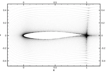
5.18 Stream-wise velocity contours for RAE2822 turbulent flow case with sub-sonic conditions. . . 43

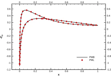
5.19 Surface pressure coefficient for RAE2822 turbulent flow case with sub-sonic conditions. . . 44

5.20 Maximum value of turbulent eddy viscosity at different vertical slices along the aerofoil for RAE2822 subsonic case. . . 44

5.21 Stream-wise velocity at different slices along the RAE2822 upper surface for subsonic case (Slices from left to right: x=1.0, x=0.9, x=0.8 and x=0.6). 45 5.22 Turbulent eddy viscosity at different slices along the RAE2822 upper surface for subsonic case (Slices from left to right: x=0.6, x=0.8, x=0.9 and x=1.0). . . 45

5.23 Pressure coefficient contours for RAE2822 case with transonic conditions. 47 5.24 Stream-wise velocity contours for RAE2822 case with transonic conditions. 47 5.25 Turbulent eddy viscosity contours for RAE2822 case with transonic con-ditions. . . 48

5.26 Maximum value of turbulent eddy viscosity at different vertical slices along the aerofoil for RAE2822 transonic case. . . 48

5.27 Stream-wise velocity at different slices along the RAE2822 upper surface for transonic case (Slices from left to right: x=1.0, x=0.9, x=0.8, x=0.6 and x=0.4). . . 49

5.28 Turbulent eddy viscosity at different slices along the RAE2822 upper surface for transonic case (Slices from left to right: x=0.4, x=0.6, x=0.8, x=0.9 and x=1.0). . . 49

5.29 Surface pressure coefficients for RAE2822 case with transonic conditions. 50 6.1 Classification of points close to an inter-processor boundary. . . 52

6.2 Algorithm for the parallel flow solver . . . 54

6.3 Algorithm for the parallel GCR . . . 55

7.1 Calculated surface pressure for Onera M6 wing case. . . 58

7.2 Comparison of computed surface pressure coefficients with PMB and experimental data at different locations throughout the wing span for Onera M6 wing at M∞= 0.86 and α= 3.06°. . . 59

7.3 Efficiency of the parallel flow solver for Onera M6 case using explicit integration with one MPI process per core. . . 60

(17)

7.5 Total number of iterations to convergence and total calculation time.

Onera M6 case. . . 61

7.6 Surface pressure contours and flow streamlines for DLR-F6 case. . . 62

7.7 Surface pressure coefficients and convergence histories for DLR-F6 case. 63 7.8 Performance of parallel solver for DLR-F6 case running one MPI process per core. . . 64

7.9 Memory usage of the parallel flow solver for DLR-F6 case. . . 64

8.1 Examples of bounding boxes over stencils and boundary elements. . . . 67

8.2 Definition of resolving vectors. . . 68

8.3 Definition of new local coordinate system for merit function. . . 68

8.4 Example of basic sorting algorithm. Smallest number for each iteration shown in light blue. Numbers already sorted shown in grey. . . 69

8.5 Domain decomposition for the preprocessor. . . 73

8.6 Example of the blanking of points interior to solid boundaries in parallel. 74 8.7 Example of a single bounding box surrounding all points assigned to a process. . . 76

8.8 Example of adaptive sub-division by quadrants on purple process (The sub-division operation and the exclusion of parents/children are shown as if they were performed together at each step). . . 77

8.9 Points identified for communication. . . 78

8.10 Example of the search region for a point. The size of the region grows with any overlapping stencil. . . 79

8.11 Representation of the hybrid MPI/OpenMP algorithm for the preprocessor. 81 9.1 Input point distributions for pitching NACA0012 test case. . . 84

9.2 Multi-Element aerofoil. . . 84

9.3 OSF test case. . . 85

9.4 Store-drop test case geometry. . . 86

9.5 Surface pressure coefficients for the NACA0012 in pitching motion. . . . 89

9.6 Normal force coefficient for NACA0012 in pitching motion. . . 89

9.7 Flow solution for multi-element aerofoil test case. . . 90

9.8 Speed-up of preprocessor for multi-element aerofoil case using distributed implementation with polar decomposition, running one MPI process per core . . . 92

9.9 Load balance for two processes for multi-element aerofoil case using dis-tributed implementation with polar decomposition . . . 92

(18)

9.11 Preprocessor memory usage for multi-element aerofoil case using

dis-tributed implementation with polar decomposition . . . 92

9.12 Number of initial and communicated points per MPI process for multi-element aerofoil case using distributed implementation with polar de-composition. Comparison of number of communication points between small and big search regions. . . 93

9.13 Performance of parallel preprocessor for multi-element aerofoil using shared and hybrid implementations. . . 94

9.14 Performance of parallel preprocessor for multi-element aerofoil using hy-brid implementation after rebalancing the partitions. . . 94

9.15 OSF test case flow solution showing surface pressure and streamlines coloured by stream-wise velocity. . . 95

9.16 Calculation times per operation, per process for OSF test case with slice-based domain decomposition . . . 96

9.17 Calculation times per operation, per process for OSF test case using polar-based domain decomposition . . . 97

9.18 Parallel preprocessor speed-up for OSF case using distributed implemen-tation with two types of domain decomposition . . . 98

9.19 Number of points received per domain for OSF case running on 12 pro-cesses. . . 100

9.20 Points per domain running on 72 processes for OSF case with distributed implementation (points received with big regions were omitted as they showed a similar trend) . . . 100

9.21 Memory usage for the OSF case using two types of domain decomposition101 9.22 Parallel performance of the hybrid (MPI/OpenMP) method for OSF case.101 9.23 Store-drop test case flow solution at t=0. . . 102

9.24 Surface pressure coefficient on the store att= 0s, measured through two different planes . . . 103

9.25 Trajectory of the store during 6-DOF simulation. . . 104

9.26 Calculated trajectory and velocities of the centre of gravity. . . 105

9.27 Calculated angular movements and rates. . . 105

9.28 Parallel performance of the method for store-drop case. . . 106

(19)

List of Tables

5.1 Flow conditions for the test cases. . . 31

5.2 Grid definition for the two-dimensional cylinder test case. . . 38

5.3 Flow conditions for the RAE2822 test cases. . . 42

5.4 Summary of force and moment coefficients for RAE2822 test cases. . . . 50

5.5 Calculation times for RAE2822 test cases. . . 50

8.1 Summary of tested sorting algorithms. . . 70

9.1 Grid sizes for the OSF test case. . . 85

9.2 Full-scale store characteristics. . . 87

9.3 Profiling of the preprocessing code. . . 87

9.4 Speed-up of different sorting algorithms. . . 88

9.5 Processor combinations in hybrid mode for multi-element aerofoil case. . 93

9.6 Preprocessor load balance for OSF test case. . . 99

9.7 Aerodynamic forces and moments at carriage position (t=0s) for store-drop test case. (All forces in N and moments in N·m) . . . 103

(20)

(21)

(22)

List of Symbols

A = Jacobian matrix (=∂R/∂w)

a = speed of sound

b,c,d = shape function derivatives

c = chord length

Cd = drag coefficient

Cf = skin friction coefficient

Cl = lift coefficient

Cm = moment coefficient

Cp = pressure coefficient

d = distance to closest wall

e = specific total energy

E = total energy

Ep = parallel efficiency

f,fv = inviscid, viscous fluxes in the xdirection g,gv ₌ _{inviscid, viscous fluxes in the} _y _direction h,hv = inviscid, viscous fluxes in the zdirection

h = specific enthalpy

i = star point

I = identity matrix

j = neighbour point

k = Cartesian direction (1=x, 2=y, 3=z)

L = level of the sub-division by quadrants

m = pseudo-time level

mp = order of polynomial

M∞ = freestream Mach number

n = unit normal vector

n = real-time level

N = number of total points in the domain p = vector of primitive variables

p = polynomial

(23)

P r,P rt = Prandtl number, turbulent Prandtl number

q = heat flux vector

R = residual vector

R = gas constant

Re = Reynolds number

Sp = parallel speed-up

t = time

T = temperature

u = velocity component in the x direction

v = velocity component in the y direction v = Cartesian velocity vector

w = velocity component in the z direction

x,y,z = Cartesian coordinates x = Cartesian coordinate vector w = vector of conserved variables

Greek Symbols

α = freestream angle of attack

αs = non-parallelisable fraction of any parallel algorithm

γ = ratio of specific heats

δ = boundary layer thickness

= tolerance

η = basis vector

τ = stress tensor

κ = thermal conductivity

µ,µt = viscosity, turbulent viscosity

˜

ν = turbulent eddy viscosity (transport variable for Spalart-Allmaras model)

ξ = vector of basis coefficients

ρ = density

φ = any function

ˆ

φ = meshless approximation to function

ψ = slope limiter

(24)

Acronyms

6-DOF = six-degree of freedom

AGARD = Advisory Group for Aerospace Research and Development BILU = block-incomplete lower–upper

CFD = computational fluid dynamics CFL = Courant-Friedrichs–Lewy DEM = diffuse element method DLR = German Aerospace Center EFG = element-free Gelerkin FEM = finite element method FPM = finite point method

GCR = generalised conjugate residual HPC = high-performance computing MIMD = multiple-instruction-multiple-data MISD = multiple-instruction-single-data MLPG = meshless local Petrov-Galerkin MLS = moving least squares

MPI = message passing interface NUMA = non-uniform memory access NS = Navier–Stokes

ONERA = French Aerospace Lab OSF = open-source fighter

PDE = partial-differential equation PMB = parallel multiblock

PML = parallel meshless

RANS = Reynolds–averaged Navier–Stokes RKPM = reproducing kernel particle method SA = Spalart–Allmaras

SISD = single-instruction-single-data SIMD = single-instruction-multiple-data SMC = symmetric multi-core

(25)

Chapter 1

Introduction

1.1 Motivation

The analysis of complex flows around bodies in relative motion is required by the aerospace industry. Example applications include the release of stores from aircraft, the opening of cavity doors, the deployment of control surfaces, helicopter blades in rotation, flapping wings, and wind turbine blades. This requirement has driven the development of numerical tools that can successfully deal with complex movable con-figurations. Conventional mesh generation techniques become difficult or impossible to apply when used to calculate flows over bodies in relative motion. For this reason, several techniques have been developed in the last few years to tackle the simulation of flow around bodies with parts in relative motion.

One technique is the meshless method, which discretises the domain by using a set of points. Each point in the domain has a sub-domain of neighbouring points, called a stencil or cloud. These clouds are then used to approximate the spatial derivatives in the partial differential equations to be solved. The meshless method is attractive for moving-body problems, as points can move independent of one another during a time-dependent simulation.

(26)

The current work documents the research carried out to implement parallel algo-rithms for the solution of turbulent flows in aerospace applications using the meshless method.

1.2 Objectives and Thesis Outline

The main aim of this thesis is the development of parallel methods applied to a meshless fluid dynamics scheme for the simulation of turbulent flows over moving geometries. Three objectives were drawn and achieved in this work.

The treatment of viscous and turbulent flows was included into an existing inviscid meshless flow solver.

Parallel computing methods were implemented for the flow solver to reduce cal-culation times.

A new parallel algorithm for the selection of stencils used by the flow solver was devised.

(27)

Chapter 2

Theoretical Background and

Literature Review

2.1 Overview of Numerical Methods for Moving

Geome-tries

Among the most commonly used techniques applied to simulating flows around moving geometry, we can name the following three methods: self-adapting grids, sliding grids, and Chimera or overset Grids. Each of them has its own advantages and disadvantages.

Self-Adapting Grids (Cartesian / Unstructured)

The foremost advantage of using self-adapting meshing is the automation that the procedure offers in grid generation. Apart from this, Cartesian or unstructured meshes in conjunction with tree data structures become a natural choice for solution-adaptive grids and dynamic flow computations involving moving bodies [1–3].

Several studies have shown the capabilities of adapting grids to compute inviscid and low Reynolds number flows [4–6]. In spite of the success involving inviscid flow computations, the main drawback of using adaptive Cartesian or tetrahedral meshes for viscous flows over complex geometries is the fact that automatically filling boundary layers with isotropic cells results in a high number of control volumes, ultimately leading to large grids [7–9].

(28)

complex geometries are too big using adaptive Cartesian or automatic triangulation techniques.

The parallel implementation of automatic grid generators has received a good amount of attention from researchers [16–21]. Several techniques like Octree sub-division, Delaunay triangulation and the Advancing-Front Technique have proven suc-cessful in dealing with different fluid problems with good parallel efficiency. The main drawback of using this type of method is still the fact that even though they are gen-erated quickly, the grids generally are not well suited for viscous and turbulent flow computations because of the increase in grid size needed to capture the flow character-istics near solid boundaries.

Sliding Grids

The concept of sliding meshes in Computational Fluid Dynamics (CFD) was first in-troduced for the analysis of turbo-machinery [22–24]. This method allows for the inte-gration of two domains (meshed separately) by interpolating the flow variables along the surface joining the two domains. Sliding meshes have been successfully used and validated in different studies where the movement between the domains is known a priori, including helicopter rotor-fuselage interaction [25, 26], turbo-machinery [27–29] and wind turbine blades [30, 31].

The sliding planes method can be implemented in parallel without much difficulty. Each separate processing unit can calculate the flow solution on its assigned data, as long as the code provides the information about the movement of cells around the sliding interface [25,32]. The main issues with this method are the interpolation needed to transfer the values from one grid to the other, and the fact that the movement of the geometry is restricted by the mating surface. This makes the method work well for problems with rotating bodies, but makes its use almost impossible for problems where the movement of the geometry is not known a-priori.

Chimera (Overset Grids)

The Chimera technique [33–35] is most often associated with finite volume/difference schemes, and its functionality is based on overlapping different grids belonging to each body or moving part. The method uses interpolations to estimate flow properties in the overlap region and besides allowing for the treatment of movable geometries, it also helps in reducing the meshing time as different parts of the domain can be meshed separately and then joined together. Normally structured grids are used with this technique.

(29)

the flow variables can be time consuming. 2) The complexity of the interconnectivity is perhaps as difficult as dealing with an unstructured grid, resulting in orphan points and bad quality of interpolation stencils [40]. 3) The fact that interpolation is generally used to connect grids implies that conservation is not strictly enforced [40].

The parallel implementation of the overset grids method is still a field of active research. Several studies have been successful at implementing the Chimera scheme in parallel [41–44]. Even so, the parallel efficiency of the connectivity methods still poses a problem. The main difficulty found is that the cost of the hole-cutting and search operations varies greatly for different regions in the computational domain, and finding an estimate of these costs to perform a correct decomposition of the domain is very difficult. In most cases, this ultimately results in low parallel efficiencies.

Meshless Methods:

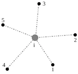
Traditional methods used in CFD (Finite Volumes, Finite Element, Finite Difference, etc) use grids or meshes as the underlying structures where the partial derivatives are discretised. Contrary to grid based methods, Meshless schemes do not require a connected grid since they can discretise the derivatives from local clouds, formed at each of the points in the domain (See Fig. 2.1). Meshless methods can be used to model problems with large geometry deformations, making them an excellent choice for applications where different bodies can interact with each other.

Although meshless methods can provide a solution for moving geometries, they are not without their drawbacks. Among the most important ones we note: 1) Finding suitable candidates to form the local clouds can be time consuming. 2) Similar to Chimera methods, by forming the local clouds of points it is possible that conservation is not strictly enforced. 3) Because of the nature of the local clouds, achieving spatial higher-order accuracy may not be as straight-forward as with traditional finite-volume methods. Even with these drawbacks, meshless methods have been shown capable of providing accurate solutions to complex problems [45, 46] and become an interesting proposition for the simulation of flows over moving geometries in aerospace applications.

(30)

2.2 Meshless Numerical Methods in Fluid Dynamics

Meshless methods for CFD is an active area of research. Important developments have been made in the last few years that have contributed to the understanding of the principles that allow the approximation functions to be built and used for solving the Navier-Stokes equations.

Main Developments Documented in the Literature

The first steps towards developing meshless methods for CFD were made almost 30 years ago. The starting point for meshless research is known as the Smoothed Particle Hydrodynamics (SPH) method and dates back to the 1970s. SPH was developed by Lucy [47] and Monaghan [48] between 1977 and 1982 to model problems in Astrophysics such as explosions of stars of particle clouds. The idea behind SPH is to replace the fluid by a set of moving particles and transforming the governing partial differential equations into the kernel estimates integrals. SPH uses a pseudo-particle interpolation method to compute smooth field variables. Each pseudo-particle has mass, Lagrangian position, velocity and internal energy. Other quantities are derived by interpolation or from constitutive relations. These particles have a spatial distance (“smoothing length”), over which their properties are “smoothed” by a kernel function. Any physical quantity is then obtained by summing the relevant properties of all the particles which lie within two smoothing lengths. Although the particles are not connected in SPH, the partitioning of the domain into volume elements is difficult, especially in three dimensions.

(31)

Parallel to the development of Lagrangian particle methods like SPH, Nayroles et al. [56] introduced the use of moving least square approximations in their Diffuse Ele-ment Method (DEM). The Diffuse EleEle-ment Method uses moving least squares interpo-lation to replace the Finite-Element Modelling (FEM) functions, valid in one element, with a weighted minimum squares approximation, valid for a small localised domain around one point [57]. The approximation function is smoothed by introducing con-tinuous functions instead of disconcon-tinuous coefficients. The fact that these weighting functions vanish at a certain distance from the main node allows for the preservation of the local character of the approximation. It can be seen that for DEM, each of the points can be considered as a particular type of finite element, with one singular integration point, a variable number of nodes and a diffuse domain of influence.

Belytschko et al. [58] then extended the idea of least squares approximation by de-veloping a method where the spatial discretisation was made by using moving least squares and a Galerkin formulation. This scheme was called Element-Free Galerkin method (EFG) and was originally devised to solve progressive crack growth in struc-tural mechanics. The method is seen as an extension of the DEM by Nayroles, and introduced two main improvements: 1) It used an auxiliary background mesh of regular cells in order to create a structure to define the quadrature points, thus allowing for the numerical integration to be performed. 2) It was able to enforce the essential boundary conditions by using Lagrange multipliers. The method showed good accuracy, as well as convergence rates which rivalled finite element methods, even though it was compu-tationally more expensive than FE models. The EFG method has found applications in many fields such as fracture, crack and wave propagation, acoustics and fluid flow [59].

An important step towards true meshless methods was the Meshless Local Petrov-Galerkin method (MLPG), proposed by Atluri et al. [60]. The MLPG method arose from the finite element community and is based on the weak form of a given PDE [61]. MLPG incorporates the moving least squares approximations for trial and test functions to discretise the local weak form of the equations. The method is based on a Petrov-Galerkin formulation in which weight and trial functions used in the discretisation of the equations do not need to be the same. This gives the method a “local” nature in which the integral is satisfied over a local domain [61]. The MLPG approach has been used successfully to solve different problems, including work on incompressible flows [62], fracture mechanics [63], and three-dimensional elasto-statics and dynamics [63].

(32)

official use of the term Finite Point Methods was provided by O˜nate [65]. He combined a weighted least square approximation of the unknowns over each local cloud with a stabilised point collocation procedure, eliminating any numerical instability. FPMs have been successfully used in several problems, including compressible inviscid and viscous flows [66, 67].

Katz and Jameson [68] developed a formal meshless scheme which compared favourably with conventional finite volume methods in terms of accuracy and efficiency for the Euler and Navier-Stokes equations. The success of their method is attributed to its local extremum diminishing property, which they generalised to handle local clouds of points instead of mesh-based schemes. The method adopts an edge-based connec-tivity to describe local points and uses Taylor series expansions with weighted least squares for the reconstruction of the gradients found in the PDEs.

Parallel Computing and Meshless Methods

Even though in recent years meshless schemes that are suitable for simulation of com-plex flows are becoming more common, most of the published work focuses on the mathematical description of the methods, without addressing the computational effi-ciency. Some researchers have implemented meshless schemes that solve the governing equations in parallel [69–72], but few have addressed the problem of parallelising the selection of local stencils. References [69, 73, 74] are among the few published works that describe the stencil selection in parallel and their method, while showing great parallel efficiency, is based on triangulation and is aimed at working on isotropic point distributions to simulate incompressible flows. To the best of the authors knowledge there has not been any published work that deals with parallel implementations for meshless schemes aimed at simulating flows over complex three-dimensional, movable geometries.

2.3 Parallel Computing Concepts

In order to simulate most scientific problems it is necessary to perform a large number of numerical computations. Historically, the desire to run increasingly complex prob-lems has been running ahead of the capabilities of the time. This has provided a driving force for the development of parallel computing. A variety of parallel computer archi-tectures have been made available during the years. One way to classify these systems is according to Flynn’s taxonomy [75]. It uses the relationship between theinstruction

stream and thedata stream to classify the four different possible architectures:

(33)

SIMD: Single Instruction stream operating on Multiple Data stream. A set of processors execute the same instruction on different sets of data. The shared memory eliminates the need for message passing constructs.

MIMD:Multiple Instruction streams operating on Multiple Data streams. These are the most versatile parallel computers. They are essentially a set of different processors that can run the same or different programs with the same or different data sets. Each processor controls its own memory and runs asynchronously. Communication between processors is accomplished via message-passing con-structs.

MISD:Multiple Instruction streams operating on a Single Data stream comput-ers are included for completeness as there are few, if any, commercial examples.

Most computers now found in scientific applications and all the machines used in this work fall into the MIMD classification. The following naming conventions for hardware components are used throughout the thesis:

Central processing unit (CPU), also referred to as “core”: the component that carries out the instructions of a program by performing the basic arithmetical, logical, control, and input/output operations of the system.

Processor: physical chip containing one or more independent central processing units. All processors used in this thesis are of the multi-core type, hence they contain two or more cores.

Computing node: self-contained computer with one or more processors.

An important sub-classification of an MIMD machine is obtained according to their memory distribution:

Shared Memory: Central processing units share a global memory space (See Fig.2.2(a)). The key feature is the use of a single address space across the whole system, so that all CPUs have access to the same view of memory. Symmetric multi-core (SMC) chips found in most modern computers fall into this category.

Distributed Memory: Processing units have their own private memory space as shown in Fig.2.2(b). Access to data assigned to other CPUs must be done through a network. Common clusters of sequential workstations with dedicated networks fall into this category.

(34)

In modern SMC systems, memory access becomes the main bottleneck as the num-ber of processing units is increased. Different CPUs would require access to the same memory space and the “system bus”, which can be thought of as a pathway between the CPUs and the memory is not big enough to transfer all the data needed by all cores at the same rate as when only one core is being used. To alleviate this problem, processor manufacturers design modern chips so that each independent core inside the chip has access to its own bus and its own memory space. This type of architectures is known as Non-Uniform Memory Access (NUMA). As these still are shared memory architectures, access to the entire memory space within the system is still possible, but cores can access their own memory space much faster than accessing the space assigned to other CPUs. For this reason care needs to be taken to ensure the data to be processed is stored locally within the space assigned to each core.

A parallel algorithm is often effective and efficient only on a specific target archi-tecture which must be carefully considered during the development. High level pro-grammers normally do not need to deal with the network topology. However, it is useful to consider a few aspects of the networks that are relevant for the design of the algorithms [76].

The standard network model involves two parameters that define the data transfer rate. The first isnetwork latency L[s], which is the time needed to initiate the connec-tion between two processing units. The second is the network bandwidth B [bytes/s], which is the rate at which data is exchanged. Because of the latency, it is better to send one long message rather than a set of short messages, even if the total amount of data to be transferred is the same.

On distributed memory machines, the communication between CPUs is made by message-passing directives. These directives have two basic types: point-to-point and global communications; respectively referring to message passing among specific cores in the system, or message passing to all cores. Message passing can also be classified

as blocking and non-blocking. Blocking messages stop execution of the code until the

(a) Shared Memory System (b) Distributed Memory System

(35)

Figure 2.3: Combined Memory System

message is received. In contrast, non-blocking messages continue with the execution of the code as soon as the communication order is issued.

There are two metrics normally used to measure the performance of parallel al-gorithms [77]. The first metric is speed-up. Speed-up indicates how much faster an application runs on p parallel CPUs compared to on one:

Sp=

T1

Tp

(2.1)

where Tp and Sp are the time the application takes and the speed-up for p cores,

respectively, and T1 is the time the application takes on one core. Often, a linear

speed-up is not possible to achieve as there is extra work involved in distributing work to the CPUs and coordinating them. In addition, an optimal serial algorithm may be able to do less work overall than an optimal parallel algorithm for certain problems, so the achievable speed-up may be sub-linear in p, even on theoretical ideal machines.

The second metric is efficiency and is given by

Ep=

Sp

p

where, Ep and Sp are the efficiency and speed-up for p cores, respectively. An

effi-ciency of 1.0 (100%) indicates that every core is being used to the full extent of its capabilities. Usually, efficiency measures that are significantly lower than 100% are due to communication overheads or the unbalanced distribution of the problem over the CPUs involved [78].

(36)

argued that the execution time can be divided between two categories: the time spent doing non-parallelisable work, and the time spent doing parallel work. Amdahl’s law argues that there is a limit to the possible speed-up based on the portion of the code that is sequential. Using this idea, the attainable parallel speed-up follows the relation

Sp =

1

β+ (1−β)

p

= p

βp+ (1−β)

where β is the portion of the code that must be computed sequentially. The time required for the sequential portion of the code is βT1, and the time required for the

parallel portion is (1−β)T1/p. It is clear that as p tends to infinity, the upper bound

for the speed-up becomesS∞= _β1.

Amdahl’s equations assume however, that the computation problem size does not change when running on an increasing number of machines, hence, the fraction of the problem that is parallelisable remains fixed. On the other hand, Gustafson noted that problem sizes grow as computers become more powerful, and that higher speed-ups than originally predicted by Amdahl’s law were in fact possible when using massively parallel machines. Gustafson’s law [80] addresses the theoretical limits introduced by Amdahl by concluding that speed-up should be measured by scaling the problem to the number of cores, and not by fixing the problem size. This approach is referred to as “weak scalability.” In Gustafson’s law the parallel speed-up is defined as

Sp=p−αs(p−1)

where αs is the non-parallelisable fraction of any parallel algorithm. Following

Gustafson’s law, an application is then called scalable if an increase in the size of the problem can be countered by a corresponding increase in the number of CPUs, and the time required for the application remains constant.

Another important concept in parallel computing is domain decomposition versus control decomposition. In domain decomposition, the domain of the input data is par-titioned and the partitions are assigned to different CPUs. In control decomposition, program tasks are divided and distributed among processing units. [77]. This decom-position is balanced if the amount of work assigned to each core is equal. The attempt to balance the decomposition is known as “load balancing” [77].

(37)

The final concept to be introduced here is the one ofthreads, which are instruction sequences that can run concurrently and are managed by the operating system at run time. Threads can be used to parallelise code on multi-core architectures as every core can execute a separate set of instructions concurrently.

2.4 Challenges of Parallel Computing Applied to

Mesh-less Methods

The problem of applying parallel computing to the meshless method is an interesting one. The meshless method starts by finding a group of neighbours (associated stencil) for each point in the domain and then, it solves the governing equations on each of these points. Finding the stencils and solving the governing equations are in fact two different problems that need to be tackled separately.

The main difficulties with the implementation of the parallel method are to correctly load balance the problem and to maintain parallel communications as well as memory consumption to a minimum. The computational cost per point for the solution of the governing equations is roughly the same for all the points in the domain. This is not the case for the selection of the stencils. All points in the domain are surrounded by other points that are possible candidates to form part of the stencils. There may be cases where some points are surrounded by only a few candidates, making the calculations for the stencil selection quite fast. On the other hand, there will be points that are surrounded by many candidates and the process of selecting the appropriate stencils is slow.

(38)

(39)

Chapter 3

Governing Equations

The Navier-Stokes equations are a system of partial differential-equations (PDEs) that define the conservation of mass, momentum and energy of fluids. They form the basis of the CFD formulation. Most aerodynamic flows are characterised by Reynolds numbers well above the critical value for transition, and thus turbulence needs to be taken into account. Viscosity plays a major role in many engineering cases and can be viewed as having two major components: a laminar one and a turbulent one. The laminar viscosity is usually a function of temperature and can be estimated using Sutherland´s formula. The turbulent viscosity depends on the mean flow characteristics and needs to be evaluated separately. In this work the turbulent viscosity is calculated by using turbulence models.

In this section we describe the mean flow equations and the Spalart-Allmaras tur-bulence model.

3.1 Navier-Stokes Equations

The motion of viscous fluids can be described by the Navier-Stokes equations. In three dimensions, the equations are written in differential conservative form as:

∂w

∂t + ∂ ∂x(f−f

v_{) +} ∂

∂y(g−g

v_{) +} ∂

∂z(h−h

v_{) = 0} _(3.1)

where w is the vector of conserved variables, f, g and h are the inviscid fluxes in the

(40)

w=                ρ ρu ρv ρw e                f =                ρu ρu2+p

ρuv ρuw

(e+p)u

               g =                ρv ρuv ρv2₊_p

ρuw

(e+p)v

               h=                ρv ρuw ρvw ρv2+p

(e+p)w

              

fv=                0 τxx τxy τxz

uτxx+vτxy+wτxz−qx

              

gv =                0 τxy τyy τyz

uτxy +vτyy+wτyz−qy

              

hv =                0 τxz τyz τzz

uτxz+vτyz+wτzz−qz

               (3.2)

Pressure is related to the conservative variables via the equation of state for a perfect gas:

p= (γ−1)

e−1 2ρ(u

2₊_v2₊_w2₎

(3.3)

The shear and normal stresses found in the viscous fluxes are:

τxx =

2

3(µ+µt) 1 Re 2∂u ∂x − ∂v ∂y + ∂w ∂z (3.4)

τyy =

2

3(µ+µt) 1 Re 2∂v ∂y − ∂u ∂x + ∂w ∂z (3.5)

τzz =

2

3(µ+µt) 1 Re 2∂w ∂z − ∂u ∂x+ ∂v ∂y (3.6)

τxy = (µ+µt)

1 Re ∂u ∂y + ∂v ∂x (3.7)

τxz = (µ+µt)

1 Re ∂u ∂z + ∂w ∂x (3.8)

τyz = (µ+µt)

(41)

qx = −

γ γ−1

1

Re( µ P r +

µt

P rt

) ∂

∂x( p

ρ) (3.10)

qy = −

γ γ−1

M∞

Re ( µ P r +

µt

P rt

) ∂

∂y( p

ρ) (3.11)

qz = −

γ γ−1

1

Re( µ P r +

µt

P rt

) ∂

∂z( p

ρ) (3.12)

whereRe, the Reynolds Number, anda, the speed of sound are defined by:

Re= ρ∞c a∞

µ∞

(3.13)

a=pγRT (3.14)

The values of γ and P r are 1.4 and 0.72 respectively in this work. In the viscous fluxes,µandµtrepresent the dynamic laminar and dynamic turbulent eddy viscosities

respectively. Here,µt is determined using the Spalart-Allmaras turbulence model and

µis determined using Sutherland’s law:

µ= µ

µ∞ =

T T∞

3/2

T∞+S∗

T +S∗ (3.15)

whereS∗ is the Sutherland constant of 110.33K for air,T∞ is the freestream tempera-ture of 255.56K for air.

The above equations have been non-dimensionalised using the following relations:

x= x

c y=

y

c z=

z

c (3.16)

u= u

u∞

v= v

v∞

w= w

w∞

(3.17)

ρ= ρ

ρ∞

e= e

ρ∞u∞

t= tu∞

c (3.18)

(42)

3.2 Turbulence Modelling (Spalart - Allmaras Model)

When simulating turbulent flows, very fine computational grids and small time-steps are needed to capture the complex flow structures that develop as the calculation pro-gresses. For most industrial applications, these requirements make the calculations infeasible for resolving all scales on the grid. Instead of solving for all the flow charac-teristics directly, an approximated solution can be calculated. One such approximation is done by modelling the effects of the small-scale motions on the computed mean-flow values (large-scale mean-flow). This approach is known as turbulence modelling for the Reynolds-Averaged Navier-Stokes (RANS) equations. In order to quantify the influ-ence of the turbulinflu-ence on the resolved flow, a closure model needs to be introduced. There are several different approaches to turbulence modelling [81,82] and usually, each of them is better suited to different applications [83–86]. The current work is aimed at simulating aerodynamic applications with compressible flows at medium to high Mach numbers. As a first approach to introducing turbulence modelling to the meshless scheme, the Spalart-Allmaras (S-A) model [87] is implemented.

The Spalart-Allmaras turbulence model solves a differential expression for the tur-bulence variable ˜ν. The model includes the treatment of transition to turbulence, but in the present study the flow is assumed to be fully turbulent. Assuming this simplifi-cation, the model in conservative dimensional form is

Dν˜

Dt =Cb1

˜

Sν˜+ 1

σ[∇ ·((ν+ ˜ν)∇˜ν) +Cb2(∇˜ν)

2_]₋_C

w1fw

˜

ν d

2

(3.19)

with the material on the left hand side derivative described as

Dν˜

Dt = ∂ν˜

∂t +v· ∂ν˜

∂x (3.20)

wherev= [u, v, w]T andx= [x, y, z]T. The term ˜νis called the turbulent eddy viscosity and contributes to the Navier-Stokes equations (Eq. 3.1) through the turbulent viscosity

µt=ρνf˜ v1 (3.21)

where the viscous damping function fv1 is given by

fv1 =

χ3 χ3₊_C3

v1

(3.22)

and χ is the ratio of the kinematic eddy turbulent viscosity to the kinematic laminar viscosity (ν =µ/ρ),

χ= ν˜

(43)

The production term is modelled by

˜

S =Sfv3+

˜

ν

κν2_d2fv2 (3.24)

fv2=

1 (1 +χ/Cv2)3

fv3=

(1 +χfv1)(1−fv2)

max(χ,0.001) (3.25)

wheredis the distance from the nearest solid wall andκ is the von Karman constant, equal to 0.41. S is the magnitude of the vorticity, written as

S=p2ΩijΩij (3.26)

where Ωij is the mean rate of rotation tensor so Eq. 3.26 becomes

S= s ∂v ∂x− ∂u ∂y 2 + ∂u ∂z − ∂w ∂x 2 + ∂w ∂y − ∂v ∂z 2 (3.27)

The values in the destruction term are

fw =g

1 +Cw33

g6₊_C w36

1₆

(3.28)

g=r+Cw2(r6−r) (3.29)

r = ν˜ ˜

Sκ2_d2 (3.30)

where Cw2 and Cw3 are constants. For large r the functionfw reaches a constant so

large values ofr can be truncated to 10.

The various constants used in the model have the following values

Cb1 = 0.1355 Cb2 = 0.622

Cv1 = 7.1 Cv2 = 5.0

Cw1 =

Cb1

κ2 +

1 +Cb2

σ Cw2 = 0.3

Cw3 = 2 σ =

2 3

(44)

To non-dimensionalise the S-A transport equation we use the same reference values as with the N-S equations, plus the following:

µ∗= µ

µ∞

, µ∗_t = µt

µ∞

, ν˜∗= ν˜ ˜

ν∞

(3.31)

where the superscript∗ denotes non-dimensional values. The superscript∗can however be dropped for convenience, and the S-A equation can be written in non-dimensional form as

∂ν˜

∂t +u ∂ν˜

∂x+v ∂ν˜

∂y +w ∂ν˜

∂z =Cb1

˜

Sν˜+ 1

σRe∞

[∇ ·((ν+ ˜ν)∇˜ν)

+Cb2(∇˜ν)2]−

Cw1fw

Re∞ ˜ ν d 2 (3.32)

where the auxiliary functions are redefined in non-dimensional form as

χ= ν˜

ν fv1 =

χ3 χ3₊_C

v13

(3.33)

fv2 =

1

1 +_Cχ v2

3 fv3 =

(1 +χfv1)(1−fv2)

max(χ,0.001) (3.34)

fw =g

1 +Cw33

g6₊_C w36

1₆

g=r+Cw2(r6−r) (3.35)

r = ν˜

Re∞Sκ˜ 2d2

˜

S=Sfv3+

˜

ν κν2_d2fv2·

1

Re∞

(45)

Chapter 4

Solution Method

4.1 Approximation of Continuous Functions from

Scat-tered Data

Scattered data approximation deals with the problem of reconstructing a function or its derivatives from given disperse data. While the idea of scattered data approximation is not new, it has recently become a fast growing area of research. For a given domain in space, discretised by a set ofN points, it is possible to define a local cloud for each of the points, as shown in Fig. 4.1. These local clouds, or stencils, are then used to approximate the required functions. In this work, the central point of each of these local stencils is referred to as the “star point” and denoted by the sub-indexi.

There are several different meshless methods that deal with interpolation from scat-tered data. A modern overview of these methods can be found in Ref. [88]. Some of the most commonly used ones include Radial Basis Functions, Moving Least Squares approximations and Reproducing Kernel Particle methods, among others. All of these methods can be used to obtain the partial derivatives of a function φ at each of the star points in the domain by interpolating scattered data from the points contained in the associated stencil of the star point. This can be written as:

∂φi

∂x =

ni X

j=0

ajφj,

∂φi

∂y =

ni X

j=0

bjφj,

∂φi

∂z =

ni X

j=0

cjφj (4.1)

whereidenotes the main point,j represents each of the points in the stencil,ni is the

number of points in the stencil with j = 0 being the star point and aj, bj and cj are

(46)

[image:46.595.209.345.91.220.2]

Figure 4.1: Local Cloud of Points.

For a functionφ(x) defined at discrete values inside the local cloud, an approxima-tion ˆφ(x) can be constructed using polynomials (p) in the form:

ˆ

φ(x) =p(x)Tα (4.2)

where

p(x) = [1 x y . . . pmp(x)]

T _(4.3)

α= [α0 α1 . . . αmp] (4.4)

In this work, the approximation to the functionφis obtained by using a first order polynomial (mp= 3):

ˆ

φ(x, y) =α0+α1x+α2y (4.5)

where the coefficients α0, α1, and α2 can be determined using a least-squares curve

fit. Performing a least-squares fit in a given cloud of points results in three equations represented in matrix form by

  

ni Σxi Σyi

Σxi Σx2i Σxiyi

Σyi Σxiyi Σyi2

  

    

α0

α1

α2

    

=     

Σfi

Σxifi

Σyifi

    

The solution of the system of equations requires the inversion of a 3 x 3 matrix which is performed for every cloud in the computational domain. Having solved these equations forα0,α1andα2, the spatial derivatives are now known since by differentiating Eq. (4.5)

it is obvious that

∂φˆ(x, y)

∂x =α1

∂φˆ(x, y)

(47)

Using this method it is possible to approximate the derivatives of any of the primitive values found in the governing equations. As an example, the derivatives of the velocity in the horizontal direction can be written as:

∂u ∂x =

ni X

j=0

α1j·u (4.6)

whereαj corresponds to the shape functionaj from equation 4.1. In addition to defining

the derivatives of the fluxes f,g and h in the governing equations, this same method can also be used to find the shear stresses and heat fluxes needed for the viscous fluxes.

4.2 Spatial Discretisation of Non-Viscous Fluxes

For inviscid flow, equation 3.1 is re-written as:

∂w

∂t + ∂f

∂x + ∂g

∂y + ∂h

∂z = 0 (4.7)

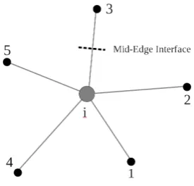
[image:47.595.249.387.459.591.2]

wherewis the vector of conserved variables, andf,gandh; are the inviscid flux vectors. This system of equations is hyperbolic in nature, hence a centered form of spatial discretisation will be unstable. In order to correctly solve the governing equations we compute upwind fluxes along the co-ordinate directions at a fictitious interface formed between the star point and each of the neighbours, as shown in Fig. 4.2

Figure 4.2: Mid-Edge Interface.

Then, the discretisation takes the form:

dwi

dt =−

ni X

j=0

a_j₋1 2 fj−

1 2 +bj−

1 2 gj−

1 2 +cj−

1 2 hj−

1 2

(4.8)

where b_j₋1 2, cj−

1

2 and dj− 1

2 are the shape functions calculated from the polynomial-least squares reconstruction evaluated at the mid-edge interface. The fluxesf_j₋1

2,gj− 1 2 and h_j₋1

(48)

appropriate entropy correction technique. Using this procedure, the mid-edge fluxes are calculated with:

f_j₋1 2 =

1

2(f(pL) +f(pR))− 1

2|A(wL, wR)|(wR−wL) (4.9) where pL and pR are the vectors of primitive values at the left and right hand side of the interface, and A is the Jacobian matrix evaluated based on the Roe’s average properties ˜W(wL, wR). For a first order accurate scheme, the vectorspLandpRsimply become:

pL=pi

pR=pj

To increase the accuracy of the solver in the presence of shocks, a higher order scheme is used. Then, the vectorspLand pR are obtained by extrapolating the values atiand j, based on a reconstructed gradient as in Ref. [45]:

pL=pi+ψij lij· ∇pi (4.10)

pR =pj−ψij lij· ∇pj

where lij is the vector formed between the star and neighbouring point, ψij is an

appropriate flux limiter, and ∇φ denotes the gradient of φ. A sufficient condition to avoid introducing oscillation in the solution process is that no new local extrema are formed during reconstruction [90]. The idea behind the slope limiters consists of finding a valueψij (∈[0,1]) in each stencil that will limit the gradient in the piecewise-linear

reconstruction of the solution. The following procedure was proposed by Barth and Jespersen [91] and is used in this work:

1. Find the largest negative (δφimin = min(φj−φi)) and positive

(δφimax= max(φj−φi)) difference between the solution in the immediate

neigh-bours and the star point in the current stencil.

2. Compute the unconstrained reconstructed value at each star point (φij = φi +

lij· ∇pi).

3. For each pointjin the stencil, compute a maximum allowable value of a function

ϕij defined as

ϕij =

      

min(1,δφimax

φij−φi), if (φij−φi)>0 min(1,δφimin

φij−φi), if (φij−φi)<0

1, if (φij−φi) = 0

(49)

4.3 Spatial Discretisation of Viscous Fluxes

The discretisation of the viscous fluxes requires a slightly different approach since they involve second order derivatives. Furthermore, the viscous fluxes in the governing equations are diffusive in nature, so a central difference scheme can be employed.

The same least squares coefficients used to discretise the partial derivatives of the Euler (inviscid) fluxes, are used to compute the gradients in the viscous fluxes. The gradients are calculated at each of the star points, so a least squares reconstruction centered at the points is used. After finding the gradients of the primitive variables, the same shape functions calculated at mid edge from the least squares coefficients are used again to calculate the second order derivatives:

∇φ= ∂φ

∂x ˆi+ ∂φ ∂y ˆj+

∂φ

∂z kˆ (4.11)

∂2_φ

∂x2 ≈ ni X

j=0

b_j₋1 2

∂φ

∂x (4.12)

To calculate the flux derivatives, simple arithmetic averages of the flow variables are used:

φij =

1

2(φi+φj) (4.13)

In the case of the second order derivatives, the averages of the gradients are modified as described in Ref. [92] to suppress the odd-even decoupling. This is:

∇φij =

1

2(∇φi+∇φj)−

1

2(∇φi+∇φj)· tij

|tij|

−φj−φi |tij|

· tij

|tij|

(4.14)

wheretij is the coordinate vector fromitojwith components{x, y, z}. As an example

of the discretisation, the derivatives of the shear stress τxy in the governing equations

can be calculated as follows:

∂(τxyij)

∂x = ∂ ∂x µ Re ∂u ∂y + ∂v ∂x ≈ ni X j=0

b_j₋1 2 µij Re ∂uij ∂y + ∂vij ∂x (4.15) where

µij =

µi+µj

2 ∂uij ∂y = 1 2 ∂ui ∂y + ∂uj ∂y − 1 2( ∂ui ∂y + ∂uj

∂y )· yij

|t_ij|−

uj−ui

|t_ij|

· yij |t_ij|

∂vij ∂x = 1 2 ∂vi ∂x + ∂vj ∂x − 1 2( ∂vi ∂x + ∂vj

∂x)· xij

|tij|

−vj−vi |tij|

· xij

(50)

4.4 Spatial Discretisation of the Turbulence Model

Equation 3.32 which describes the Spalart-Allmaras model can be re-written in similar manner to the Navier Stokes treatment above, after some algebraic manipulation. This means separating the equation into a time derivative, convective and diffusive terms plus an algebraic source term:

∂ν˜

∂t +

ConvectiveT erms

z }| {

∂(H)

∂x + ∂(I)

∂y + ∂(J)

∂z =

Dif f usiveT erms

z }| {

1

Re

∂(Hd)

∂x + ∂(Id)

∂y + ∂(Jd)

∂z + SourceT erm z}|{ K (4.16) where

H =uν,˜ I =vν,˜ J =wν˜

Hd= ν+ ˜ν

σ

∂ν˜

∂x

, Id= ν+ ˜ν

σ

∂ν˜

∂y

, Jd= ν+ ˜ν

σ

∂ν˜

∂z

The algebraic source termK can be divided into four components as follows:

K=K1+K2+K3+K4 (4.17)

K1 = Cb1S˜ν˜

K2 =

Cb2

σRe∞ "

∂ν˜

∂x

2 +

∂ν˜

∂x

2 +

∂ν˜

∂x

2#

K3 = −

Cw1fw

Re∞ ˜ ν d 2

K4 = ν˜

∂u ∂x + ∂v ∂y + ∂w ∂z

(51)

dwi

dt =−

ni X

j=0

b_j₋1 2 (fj−

1 2 −f

v

ij) +c_j−1 2 (gj−

1 2 −g

v

ij) +dj−1 2 (hj−

1 2 −h

v

ij)

−Ki

(4.18) where the convective and diffusive terms in the Spalart-Allmaras equation are added to the inviscid and viscous fluxes respectively, and the algebraic source term is included in the right-hand side of the equation.

4.5 Boundary Conditions

Ghost points located outside of the boundary elements are used in order to impose boundary conditions along the geometry. The location of these ghost points is de-termined by reflecting the flow field points that are close to the surface, as shown in Fig. 4.3.

Figure 4.3: Ghost Points

For inviscid flow, “slip conditions” are enforced on solid walls by setting the variables at the ghost points so that the velocity normal to the boundary is zero:

u·n= 0

For viscous flows it is necessary to enforce a “no-slip condition” at the solid walls. This is achieved by setting the tangential velocity on the boundary wall to equal the wall velocity. Considering a static wall, this means u = 0. For the Navier-Stokes equations, the velocity values at the ghost point must have the opposite value to that of its equivalent interior point.

ug=−ui, vg=−vi, wg =−wi

(52)

order extrapolation of the values at the interior and surface points. At the far field, the ghost points have the values of the freestream quantities.

For the turbulence model, the turbulent eddy viscosity at the surface walls is set to zero (˜ν = 0). At the freestream, ˜ν depends on the freestream kinematic laminar viscosity (ν∞). Values of ˜ν∞≤0.1ν∞ are acceptable [87].

4.6 Integration to Steady-State

Once the spatial discretisation has been calculated, the time integration is performed. It is helpful to first write Eq. (4.18) in terms of a residual:

∂w

∂t =−R(w)i (4.19)

As a first integration stage a simple explicit forward difference iteration in pseudo-time (ς) is used to smooth out the initial flow field:

∆w=wm+1−wm (4.20)

wm+1=wm−∆ςR(wm) (4.21)

where R(w) is the residual vector, consisting of the right-hand side of Eq. (4.8) and the superscript mdenotes the time level in pseudo-time ς.

In order to increase the rate of convergence an implicit integration scheme is used:

∆w

∆ς =−R(w

m+1₎ _(4.22)

This represents a system of non-linear algebraic equations. In order to simplify the solution procedure the residualR(wm+1) is linearised as follows:

R(wm+1) = R(wm) +∂R(w)

∂ς ∆ς+O(∆ς

2₎ _(4.23)

≈ R(wm) +∂R(w)

∂p

∂ς∆ς (4.24)

≈ R(wm) +∂R(w)

∂p ∆p (4.25)

where p is the vector of primitive variables, ∆p = pm+1 −pm, and ∂_∂R_p is the flux Jacobian matrix with respect to the primitive variables at each point. Choosing a Jacobian with respect to primitive variables makes the differentiation simpler.

After linearising the flux residualRm+1in pseudo-time, Eq. (4.22) becomes a system of linear equations to be solved for the primitive variablesp.

I ∆ς

∂w

∂p +

∂R

∂p

(53)

where ∂_∂w_p is the transformation matrix between conservative and primitive variables.

For the solution of this system to steady-state, an approximate form of the Jacobian matrix with a sparsity pattern from a first order spatial discretisation is used. The linear system is solved by using an iterative solver with a preconditioner based on block incomplete lower-upper (BILU) factorisation [93]. The size of ∆ς is determined by a local time-step estimate [68] in order to accelerate convergence to a steady-state.

4.7 Iterative Linear Solver

As mentioned before, an iterative method is used to solve the linear system described in Eq. (4.26). The method is based on successive approximations to the solution of a system:

Ax=b (4.27)

whereAis the coefficient matrix,bis the right hand side andxthe vector of unknowns. The basic successive approximation approach is worked out by defining a residual vector as r = b−Ax. The method used for the solution of the system is the Generalised Conjugate Residual algorithm (GCR) [94, 95], which is shown in Algorithm 1.

Algorithm 1 GCR

1: Compute r0 =b−Ax0. Setp0 =r0. 2: Forj= 0,1, ..., until convergence, Do:

3: αj = ₍(_Aprj_j,Ap_,Apj_j)₎ 4: xj+1=xj+αjpj 5: rj+1=rj−αjApj

6: Compute βij =−(Ar₍_Apj+1,Api)

i,Api) , fori= 0,1, ..., j

7: pj+1=rj+1+ j

P

i=0

βijpi 8: EndDo

To compute the scalarsβij in the algorithm, the vectorArj and the previous Api’s

are required. In order to limit the number of matrix-vector products per iteration to one, we can proceed as follows: Follow line 5 by a computation of Arj+1 and then

computeApj+1 after line 7 from the relation:

Apj+1=Arj+1+ j

X

i=0

βijApi

4.8 Preconditioning

(54)

the original linear system into an equivalent system having the same solution, but that is easier to solve with an iterative solver. Numerically, the preconditioner is a non-singular matrix (M) with the property that the system M x = b is less expensive to solve than the originalAx=b. After applying the preconditioner, algorithm 1 becomes:

Algorithm 2 Preconditioned GCR

1: Compute r0 =M−1(b−Ax0). Setp0 =r0. 2: Forj= 0,1, ..., until convergence, Do:

3: αj =

(rj, Apj)

(Apj, M−1Apj) 4: xj+1=xj+αjpj 5: rj+1=rj−αjM−1Apj 6: Compute βij =−

(Arj+1, Api)

(Api, M−1Api)

, fori= 0,1, ..., j

7: pj+1 =rj+1+ j

P

i=0

βijpi 8: EndDo

4.9 Time-Accurate Integration

For time-accurate, unsteady simulations, Eq. (4.22) must be solved in real-timet, such that

dw dt =−R

n+1 _(4.28)

where the superscript n denotes the time level in real-time t. The time integration is done using Jameson’s dual time-stepping method [96], in which Eq. (4.28) becomes

R∗ = 3w

n+1₋_4wn₊_wn−1

2∆t +R

n+1_{= 0} _(4.29)

whereR∗ is defined as the unsteady residual. This is a non-linear system of equations that cannot be solved directly. Instead, Eq. (4.29) can be viewed as a modified pseudo-time steady state problem, which can be solved iteratively for wn+1 by introducing a derivative with respect to the fictitious pseudo-timeς, as explained in Ref. [45]. Finally, the following system for the updates is obtained:

1 ∆ς +

3 2∆t

∂w

∂p +

∂R

∂p

∆p=−

3wm−4wn+wn−1

2∆t +R

m

Development of parallel meshless methods for moving geometry simulations