Identifying friction stir welding process parameters through coupled
numerical and experimental analysis
Xingguo Zhou, Wenke Pan
*, Donald MacKenzie
University of Strathclyde, 75 Montrose Street, Glasgow G1 1XJ, UK
Keywords:
Friction stir welding Genetic algorithm
Automatic parameter identification Numerical modeling
Python
a b s t r a c t
Friction Stir Welding (FSW) is a complex thermal-mechanical process. Numerical models have been used to calculate the thermalfield, distortion and residual stress in welded components but some modeling parameters such asfilm coefficient and thermal radiation of the work pieces may be technically difficult and/or expensive to measure experimentally. Therefore, it is important to establish a systematic pro-cedure to identify FSW process parameters. In this paper, a simplifiedfinite element model for analysis of a FSW thermal progress is proposed in which two parameters, tool heat input rate and heat loss through the backing plate, are identified as parameters for optimization through application of a generic algo-rithm. A genetic algorithm is used to evaluate the two thermal parameters. By comparing the FEM numerical results with experimental results, the FSW process thermal parameters have been successfully identified. This automatic parameters characterization procedure could be used for the FSW process optimization.
Ó2013 Published by Elsevier Ltd.
1. Introduction
Invented in 1991 by The Welding Institute, Friction Stir Welding is an advanced welding technology for joining materials in solid state. Compared to conventional fusion welding, FSW can achieve good weld mechanical properties and it is especially suitable for welding high strength aluminum. FSW is not only a user friendly process but also an environmentally friendly process because it doesn’t emit toxic gases nor UV rays which are harmful to human health. Furthermore, low residual stress and distortion is expected, making the technique attractive for welding large sheet material.
FSW was initially developed for joining low-weldability aluminium alloys, but has since been used to join a variety of mate-rials in a range of industry sectors.Fig. 1shows a schematic drawing of a FSW tool and workpiece. The whole FSW process involves four stages: plunge, dwell, traverse and retraction. A cylindrical pin with a larger shoulder rotates and gradually plunges to a certain depth into the material and then dwells for certain time to let the workpiece temperature reach the optimal welding temperature, then traverses with constant speed along the weld line to thefinish point andfinally retracts from the workpiece.
The temperature history plays a very important role in final grain size and distribution and dissolution of precipitates and
consequently affects the mechanical properties of the weld. By using the Rosenthal equation, Gould[1]investigated the temper-ature distribution of FSW workpiece with the assumption that heat was solely generated by the work done by the friction force between the workpiece and tool shoulder. Vilaca et al.[2]also used the Rosenthal equation to deduce the analytical solution for ther-mal distribution formulation by placing the point heat source at the middle plane along the thickness direction of the workpiece and considered the heat generated from not only the translation but also the rotation movement of the welding tool.
Apart from the simplified analytical thermal solution of FSW, different types of numerical thermal modeling methods were also studied by researchers. Chao [3] et al. initially presented a 3-D thermal model including heat generation from the shoulder. Later, they used an inverse method to obtain the thermal param-eters with the analysis of the separated models of workpiece and tool[4]. In Colegrove’s model[5], heat generated from shearing of the material and friction on the vertical and threaded surface of the pin were studied. By correlating the heat input with the experi-mentally measured torque and considering different types of con-tact conditions including sliding, sticking and partial sliding/ sticking, a 3-D thermal model was analyzed by Khandkar et al.[6]A detailed review on the simplified FSW thermal model can be found in Ref.[7].
However, as FSW is a complicated thermal-mechanical process, some modeling parameters such as film coefficient and thermal radiation of the work pieces may be technically difficult and/or *Corresponding author. Tel.:þ44 01415482036.
E-mail address:[email protected](W. Pan).
Contents lists available atSciVerse ScienceDirect
International Journal of Pressure Vessels and Piping
j o u r n a l h o me p a g e : w w w . e l s e v i e r . c o m / l o ca t e / i j p v p
expensive to measure experimentally. Previous research work on numerical FSW thermal modeling mainly focused on trial and error methods to obtain these thermal parameters. This may be very time consuming or difficult to obtain optimal values. Therefore, it is important to establish a systematic procedure to identify FSW process parameters.
In this paper, an automatic FSW process for thermal parameters characterization is presented. For validation of the proposed method, experiment results from Ref.[4]are used for comparison. In the following section, a brief introduction of how ABAQUS Py-thon commands are used to manage a high performance cluster by allocatingfinite element jobs to different nodes to perform parallel simulation is given. An investigation of a basic finite element thermal model, which was used for the thermal parameters iden-tification in the later simulation, is presented. Section4is about the genetic algorithm for optimization of thermal parameters, while in Section5, the results are given. Thefinal section is the conclusions and further work.
2. ABAQUS python scripts for parallel simulation
The identification process for FSW parameters includes: (1) to build a trial FEM thermal model with guess values for the param-eters to be identified (2) to employ a genetic algorithm (GA) method to obtain the optimal values for these parameters (3) to use high performance clusters for the simulation of FEM model with the parameters updated by GA procedure. Due to the large amount of FEM modeling involved, a systematic procedure has to be developed. The proper use of ABAQUS python scripts could provide an ideal way to deal with this problem. Before the start of the ABAQUS python procedure, a basic FEM thermal model will be established (see Section3). The FEM results will be compared with that of the theoretical results and the model with good results will be kept for the later simulation.Fig. 2shows theflow chart used for thermal parameters optimization. Firstly, the basic ABAQUS model file is called and the heat input and surface film coefficient user subroutines are prepared. Secondly, the GA module is called to modify the thermal parameters in user subroutines. Each GA gen-eration consists of 20 seeds, therefore, 20 FEM models are prepared.
Thirdly, 20 different ABAQUS jobs are allocated and submitted to different HPC nodes. Fourthly, after these jobs havefinished, the ABAQUS post-processing program is called to extract the temper-ature history data at the points of interest for all the models. By comparing the calculated results with that of experimental results, the whole procedure will stop if the convergence criterion is satisfied or the total iteration number reached. Otherwise, go to second step and repeat the second step to fourth step until the defined criterions satisfied.
3. FSWfinite element thermal model
To validate the proposed FSW process thermal parameters identification method, the FSW experiment results from Ref.[4]are used for comparison. In ref. 4, two aluminum plates of length of 610 mm, width 102 mm and thickness 8.1 mm are friction stir welded. The case with tool traverse speed of 2.36 mm/s is studied in this paper. The thermal history data at the point (named as Point C for convenience) 5 mm from the weld line on top surface is used for thermal parameter characterization, while the temperature varia-tion with time at another point (named as point D) on middle plane of the plate with same distance as point C from the central line is employed for validation.
To obtain the optimized values for the FSW thermal parameters, large numbers of FEM models has to be analyzed. Because only the thermal parameters are to be identified, a basic FEM model will be analyzed and then this model will serve as a model for other sim-ulations. The only change for other models is the modification ofQ1 andQ2 (seeFig. 1) and their values can be written into the models through ABAQUS user subroutines.
3.1. Basic thermal model
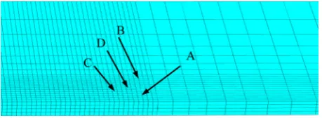
[image:2.595.323.553.66.150.2]Fig. 3shows a simplified FSW 3D transient thermal model with a continuous point heat source applied at point A, i.e. the centre point along the welding line. As two identical aluminum plates are to be welded, a half model is analyzed. The ABAQUS 3D 8-node brick element is employed and the model contains 19,215 nodes and 14,560 elements. The material thermal conductivity and specific heat are taken from Ref.[4]. Assuming no heat dissipation from the Fig. 1.Schematic drawing of FSW tool and workpiece:Q1 presents heat input,Q2
presents heat dissipation to support plate.
No
Yes
Start
Call genetic algorithm module
and modify the user subroutines
to obtain FEM models
Post-process all FEM model data and extract
thermal history info at the interested points
End
Criterion satisfied?
Basic
ABAQUS
thermal model
Allocate and submit FEM jobs
to different HPC nodes for
[image:2.595.50.283.67.164.2]parallel simulation
Fig. 2.ABAQUS python procedure for parameters optimization.
[image:2.595.108.494.638.729.2]workpiece, the numerical results can be compared with analytical solution where a point heat source is applied to an infinite plate. The analytical temperature formulation for any point at timetis given as follows[8].
T
R;t
¼ 2q
pl
R1
F
R ffiffiffiffiffiffiffiffi 4at p (1)
where the heat rateq, conductivity
l
, specific heatcand densityr
are 1000w, 120w/m2, 1000w/m3 and 2700 kg/m3 respectively.
Whilea¼
l
=ðc*rÞ
andFð
uÞis the probability integral function.Ris the distance from the heat source,tis time in second.Fig. 5is the comparison of the temperature history between the numerical and theoretical results at point B (10 mm from point A along the line perpendicular to the weld line). From thisfigure, it can be seen that the numerical results are in good agreement with that of the analytical results within 1.1 s, but with the time in-creases, the error becomes bigger. This error is mainly because the heat can be accumulated in the numerical model with small thickness, while for the theoretical model the heat can be trans-ferred to the far area. The error is not caused by the mesh and integration step time, therefore this model serves as a basic model for the later simulation.
3.2. FSW FEM model for thermal parameters characterization
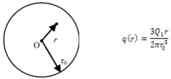
The thermal model for FSW is based on the basic thermal model. Instead of a continuous point heat source, a moving heat source with a constant total heat input rateq(r) labeled asQ1 in Equ.2, to be identified, from the tool shoulder is assumed, but the heat input rate for each point under the shoulder will be proportional to the distance (r) from the point to the centre of the shoulder, as shown inFig. 4, wherer0is the radius of the tool shoulder.
The heat transferred from the workpiece to the support plate is considered through a thermalfilm coefficient, defined asQ2 with uniform distribution, to be identified. The advantage of introducing Q2 is that there is no need to include the support plate into the plate. Hence, the total CPU time for the simulation will be reduced.
qr ¼ 3Q1r 2
p
r3 0(2)
[image:3.595.72.244.65.144.2]The heat dissipated from the side and the top surface of the workpiece to air is considered through the use of thermal film coefficient with a value of 30w/m2in the FE model. Due to sym-metry, no heat exchange occurs on the middle plane along the weld line. The initial temperature for the whole workpiece is assumed to be 25C. Material properties, including specific heat and conduc-tivity, are assumed to vary with temperature, and are listed in
Table 1andTable 2respectively[4].
4. Genetic algorithm for thermal parameters characterization
Based on the natural rule offitter creatures having more chance to survive, GA is one type of optimization method especially suitable for parallel simulation. In this paper, the optimal values forQ1 andQ2 are to be identified. In using GA,Q1 andQ2 will be represented by an integral (with 8 bits of 0 and 1) with the range of 0e255. The real values ofQ1 andQ2 can be calculated from the integral using the formulation shown inFig. 6with a given range forQ1 andQ2, vice versa. In this case, searching ranges forQ1 andQ2 are assumed as [1000w, 2000w] and [100w/m2/C, 500 w/m2/C] respectively.
Theflow chart of GA process is shown inFig. 7. Initially, 20 sets of chromosomes corresponding toQ1 andQ2 are randomly generated. Then the real values ofQ1 andQ2 are calculated. Follow this, 20 FEM thermal model jobs are prepared and submitted to the HPC. After the solutions are complete, the temperature history data is extracted at the points of interest such as pointCandDdefined in Section3.1.
This will follow the calculation of the value of the objective function
d
for each seed, defined as:d
¼ffiffiffiffiffiffiffiffiffiffiffiffiffiffiffiffiffiffiffiffiffiffiffiffiffiffiffiffiffiffiffiffiffiffiffiffiffiffiffiffiffiffiffiffi 1
n
Xn
i¼1
Ti
calTexpi
Ti exp !2 v u u u t (3)
[image:3.595.39.279.536.726.2]Fig. 4.Heat input rate distribution under the tool shoulder.
Fig. 5.Comparison of temperature result between FEM and analytical model.
Table 1
Conductivity property of workpiece[4].
Conductivity 90 100 110 120 130 140 150
Temperature 0 50 100 150 200 250 300
Table 2
Specific heat of workpiece[4].
Specific heat 900 1000 1077 1100
Temperature 0 150 250 300
[image:3.595.303.539.583.730.2]Q1 1000 ... ... ... 2000 0 ... ... ... 255 (Q1-1000)/(2000-1000)X255 1000+K1/255X(2000-1000) K1
whereTi
expandTcali are the experimental and calculated tempera-ture for theith seed respectively.‘n’ represents the total points extracted from the temperature vs time curves. Thefitness for each seed is defined asf ¼1=
d
, and the largest value offitness in one generation is selected as thefitness of the generation. Finally, if the value ofd
is smaller than a given small value or the total number of generation is larger than 100, the GA process stops. Otherwise, new off-spring for next generation will be created through selection, cross-over and mutation. These steps are repeated until the crite-rion is satisfied.5. Numerical results
Based on the GAflowchart shown in Fig. 7 and the ABAQUS
Python procedure shown inFig. 2, both the GA module and ABAQUS Python codes are developed. The temperature history[4]at point C (see Section3) are divided into 20 segments as shown inFig. 7, therefore 21 experiment data points are used for calculating the GA objective function value.
The data points were chosen purposely after 100 s of welding because the temperature is not sensitive to the welding time at an earlier stage. After GA evolution to the 35th generation, the average
relative error between the experimental and numerical results is smaller than 5%. The values for the thermal parametersQ1 andQ2 obtained are 1714W and 462W/m2. By using these identified param-eters and performing ABAQUS simulation again, the comparison of
No
Yes
No
Yes
Start
Initialization: assign values for Q1 and Q2
randomly. Total 20 seeds are generated.
Perform 20 FEM model simulations by HPC,
extract thermal history information
Calculate the objective function & fitness for all
seeds and find the best in current generation
Produce next generation seeds via
selection, crossover & mutation
Rank seeds according to fitness
Generations >100 ?
>
0 [image:4.595.146.461.69.218.2]End
Fig. 7.GAflow chart for identification of FSW process thermal parameters.
[image:4.595.323.550.254.453.2]Fig. 8.Comparison of experimental[4]& predicted temperature at point C.
Fig. 9.Comparison of experimental[4]& predicted temperature at point D.
[image:4.595.49.289.511.726.2] [image:4.595.313.560.537.728.2]experimental and numerical results at point C is shown inFig. 7. This shows good agreement between the results of the two methods. The thermal history at another point D is also predicted and depicted in
Fig. 9. A similar conclusion can be made as that fromFig. 8. This comparison shows that the proposed numerical model is reliable and accurate because the measured temperature data at point D has not been included into the thermal parameters characterization proce-dure. InFig. 10the relative error between the predicted and experi-mental results is plotted against GA iteration number.
6. Conclusions and future work
Taking advantage of high performance cluster parallel computing and the commercial Finite Element software ABAQUS python codes, the Finite Element Method was coupled with a genetic algorithm optimization to obtain the best value for the thermal input (heat from a moving heat source simulating friction stir welding) and thermalfilm coefficient (between the workpiece and support plate). By using the predicted parameters from one set of experiment results, the temperature distribution at other points are predicted and found to be in good agreement with the experimental results. The heat input predicted is also similar to that obtained in Refs.[4], in which a general inverse method is used. The optimization pro-cedure presented in this paper performs the parameter identifi ca-tion automatically and could be extended to include the complex features of the welding tool. As the temperature history plays a very important part of the microstructure in welded zones, this
systematic procedure could be used for FSW process optimization. Future work will include the thermal mechanical coupling analysis to predict the residual stress and distortion.
Acknowledgments
The authors would like to thank Scottish Overseas Research Student Awards Scheme and University of Strathclyde forfinancial supporting the research.
References
[1] Gould J. Heatflow model for friction stir welding of aluminum alloys. J Mater Process Manuf Sci 1998;7:185e94.
[2] Vilaca P, Quintino L, Santos JF. iSTIR-analystical thermal model for friction stir welding. J Mater Process Tech 2005;169(3):452e65.
[3] Chao YJ, Qi X. Thermal and Thermo-mechanical modelling of friction stir welding of aluminum alloy 6061-T6 plates. J Mater Process Manuf Sci 1998;7: 215e33.
[4] Chao YJ, Qi X, Tang W. Heat Transfer in friction stir welding-experimental and numerical Studies. J Manuf Sci Eng 2003;125:138e45.
[5] Colegrove P. 3-Dimentional Flow and Thermal Modelling of the Friction Stir Welding Process. Proceedings of the 2nd International Symposium on Friction Stir Welding, Sweden, August 2000.
[6] Khandkar MZH, Khan JA, Reynolds AP. A Thermal Model of the Friction Stir Welding Process’, Proceedings of IMECE2002, ASME International Mechanical Engineering Congress & Exposition, New Orleans, Louisiana, November, 2002. [7] Li HJ. Coupled thermo-mechanical modelling of friction stir welding. PhD
thesis. UK: University of Strathclyde; 2008.
![Fig. 9. Comparison of experimental [4] & predicted temperature at point D.](https://thumb-us.123doks.com/thumbv2/123dok_us/1670245.120549/4.595.49.289.511.726/fig-comparison-experimental-predicted-temperature-point-d.webp)
