Spectral schemes on triangular elements
by Wilhelm Heinrichs and Birgit I. Loch
Abstract
The Poisson problem with homogeneous Dirichlet boundary conditions is considered on a tri-angle. The mapping between square and triangle is realized by mapping an edge of the square onto a corner of the triangle. Then standard Chebyshev collocation techniques can be applied. Numerical experiments demonstrate the expected high spectral accuracy. Further, it is shown that nite dierence preconditioning can be successfully applied in order to construct an ecient iterative solver. Then the convection-diusion equation is considered. Here nite dierence pre-conditioning with central dierences does not overcome instability. However, applying the rst order upstream scheme, we obtain a stable method. Finally, a domain decomposition technique is applied to the patching of rectangular and triangular elements.
Keywords
spectral, collocation, triangle, preconditioning, Poisson, convection-diusion, domain decompo-sition.
Introduction
Pseudospectral collocation methods give good approximations to smooth solutions of elliptic par-tial dierenpar-tial equations. However, there is a huge disadvantage as these methods are conned to rectangles. Additionally, the spectral operator is ill conditioned compared to nite dierence or nite element operators and requires preconditioning to construct an eective iterative solver. Here, we apply the standard Chebyshev collocation method for solving partial dierential equa-tions on certain right triangles. We introduce a transformation between the triangle and the standard square where spectral collocation can be applied. This transformation maps one edge of the square onto one corner of the triangle so that the non-equally spaced collocation points cluster in that corner. In [6] a dierent approach has been examined. The results are compared. This method is then applied to the Poisson equation with homogeneous Dirichlet boundary conditions on a right triangle. It is numerically shown that for smooth solutions high spectral accuracy can be achieved. Then we introduce a singularity caused by the singular behaviour of the right-hand side leading to a somewhat slower convergence of the approximation. Precondi-tioning by nite dierences yields a condition number increasing as O(N).
After that the convection-diusion equation is considered. To overcome the instability for small
we choose N to be odd (see [1]). Preconditioning by central nite dierences yields an un-bounded condition number such that an upwind method has to be applied.Transformation of the right triangle
The standard Chebyshev collocation scheme (see [6]) is dened for the non-equally spaced Chebyshev-Gauss-Lobatto nodes (
s
i;t
j) = (cosiN;
cosjN) on the square [ 1;
1]2. Usinglin-ear transforms, arbitrary rectangles can be considered. However, if we are interested in tri-angular domains the mapping is more complicated. In [6] a mapping applying polar coor-dinate transformation and bending of an edge of the triangle was introduced and analyzed. Numerical results showed the eectiveness of this method. Here we consider a new transfor-mation between the standard square
R
= f(x;y
) j 1< x;y <
1g and the right triangleT
= f(x;y
) j 0< x;y <
1 andx
+y <
1g. The original mapping is given in [7] and has beenchanged for our purposes. The transformation reads
x
= 14(
x
R+ 1)(1y
R); y
= 12(
y
R+ 1)x
R = 2x1 y 1
;
y
R= 2y
1and is displayed in Figure 1.
6
-@ @ @ @ @
x
y
1
-1 -1
1
T
6
-x
Ry
R@ @
@ @
@ @
@ @
@ @
@ @
1
-1 -1
1
Figure 1: Horizontal transformation
We will call this the horizontal transform as every node is actually moved horizontally. The vertical transform is
x
= 12(
x
R+ 1); y
= 14(
y
R+ 1)(1x
R)x
R = 2x
1;
y
R= 2y 1 x 1and will be considered later.
Partial derivatives must be transformed, too. Using the horizontal transform we derive
u
x = 2u
x1 = 4 1 yRu
xRu
xx = 4u
x1x1 = 16 (1 yR)2
u
xRxRu
y = 2u
y1 = 2xR+1
1 yR
u
xR+ 2u
yRu
yy = 4u
y1y1 = 4 (xR+1)2 (1 yR)
2
u
xRxR + 8xR+1
1 yR
u
xRyR+ 8xR+1 (1 yR)
2
u
xR+ 4u
yRyR:
The Laplacian then reads as follows
u
=u
xx+u
yy= 44+(xR+1) 2 (1 yR)
2
u
xRxR + 8xR+1
1 yR
u
xRyR+ 8xR+1 (1 yR)
2
u
xR+ 4u
yRyR:
The Poisson problem
Numerous spectral algorithms for the numerical simulation of physical phenomena demand the approximative solution of one or more Poisson problems in a bounded domain.
We now study the problem
u
=f
inT;
u
= 0 on@T;
where
@T
denotes the boundary of T. We apply the standard Chebyshev collocation scheme to the exact solutionu
(x;y
) =xy
(e
x+ye
):
(1)This function obviously fullls the boundary condition. Table 1 shows the discrete L2 error E2 :=
ku uNk 2
N . One observes the exponential decay of the
error.
N
E
2 E2 in [6]4 1
:
94105 1
:
89 104
8 2
:
041011 8
:
85 107
16 2
:
121016 1
:
84 1011
32 4
:
291016 1
:
78 1016
Table 1: Error using horizontal transformation and [6]
-6 @ @ @ @ @ @ @ @ @ 1 1
y
x
6-x
1y
1 1 -1 -1 1Figure 2: Positions of the Chebyshev collocation nodes for
N
= 16Comparison of these results to those in [6] using polar coordinate transformation (see Table 1) shows that our mapping yields a faster convergence of the approximation. Here rounding error accuracy is already reached for N=16. N=4 and N=8 give results which are more exact by 1 or 5 digits. This can be explained by the position and way of numbering the collocation nodes. Figure 3 shows that the jumps occuring when changing the row (e.g. from third to fourth point) are decreasing while those in [6] seem to be larger. The speed of convergence is probably inuenced by greater jumps.
@ @ @ @ @ @ @ @ @ 3 2 1 4 5 6 7,8,9 @ @ @ @ @ @ @ @ @ 1 2 3,6,9 4 5 7 8
Figure 3: Order of collocation points for
N
= 2 compared to [6]Next we consider a singular problem where
f
1. We compare the results for N=4, 8, 16and 32 to those obtained for N=36 at the xed points displayed in Figure 4. These points are the collocation nodes for N=4 which are also used for larger N divisible by 4. We expect the error to be smallest close to y=1 because there the collocation nodes cluster. We deal with the following nodes:
P
(0;
0); P
(p;
p)
; P
( p;
p)
; P
(p;
p) and
P
( p;
p-6
@ @
@ @
@ @
@ @
@
1 1
y
x
6
-x
1y
11
-1 -1
1
P
1
P 4
P
2
P 3
P 5
Figure 4: Positions of the ve nodes
The approximation converges more slowly than in the last example. That makes sense because here the dierential equation and its boundary condition are not compatible any more.
To get an overview we present
ER
=ju
Nu
36jwhich is the absolute value of the dierence for
every node, in a diagram (Figure 5).
1e-12 1e-11 1e-10 1e-09 1e-08 1e-07 1e-06 1e-05 0.0001
5 10 15 20 25 30
ER
N
P1 P2 P3 P4 P5
Figure 5: Poisson problem with constant
f
Next we choose f discontinuous:
f
(x;y
) =(
1 for
y x >
0 0 fory x
0:
As Figure 6 shows the triangle is now bisected. The transformation of the line
y
=x
on the triangle gives the hyperbolay
= 2x+1-6
@ @
@ @
@ @
@ @
@
1 1
y
x
f =0 f = 1
6
-x
1y
11
-1 -1
1
f = 1
f =0
Figure 6: Transformation of the line
The results can be found in Figure 7.
1e-08 1e-07 1e-06 1e-05 0.0001 0.001 0.01
5 10 15 20 25 30
ER
N
P1 P2 P3 P4 P5
Figure 7: Poisson problem with discontinuous
f
The approximation is relatively bad close to the separating line. Since f is discontinuous the solution of the partial dierential equation is no longer smooth and there is no high spectral accuracy any more. We only have a rst order method.
Preconditioning
We are interested in a good condition number of our spectral operator which does not increase too fast such that ecient iterative solvers can be found. Here the maximum eigenvalues of the spectral Laplacian on the triangle scale as
O
(N
8) (Table 2). On the square one hasO
(N
4) whichreduced if we multiply the operator by (1
y
R)2 . The partial derivatives contain this factor inthe denominator. For y close to 1 the inuence of the appropriate partial derivative is extremely high. The discretized operator is called
L
2;SP. Table 3 showsmax:=max
fj
jjeigenvalue
g, min:=min
fjjjeigenvalue
g andcond
maxmin. Here the condition number scales as
O
(N
4).N
max mincond
max=N
84 5
:
39103 5
:
36 101 1
:
01 102 0
:
088 1
:
10106 4
:
94 101 2
:
23 104 0
:
0716 2
:
71108 4
:
93 101 5
:
49 106 0
:
0632 6
:
861010 4
:
93 101 1
:
39 109 0
:
06Table 2: The spectral operator
L
SPN
max mincond
max mincond
4 6
:
36102 5
:
41 101 1
:
18 101 1
:
15 102 5
:
10 2:
26 101
8 9
:
77103 5
:
35 101 1
:
83 102 1
:
89 103 4
:
58 4:
15 102
16 1
:
56105 5
:
32 101 2
:
94 103 3
:
07 104 4
:
39 7:
00 103
32 2
:
50106 5
:
30 101 4
:
71 104 4
:
93 105 4
:
29 1:
15 105
Table 3: The spectral operator
L
2;SP and results in [6]
Our results are comparable to those in [6].
We now study the nite dierence preconditioner
L
FD which is the discretization of theLapla-cian by second order nite dierences. The rst and second derivatives are
w
0(s
j) = 12(
j 1w
(s
j 1) (j j 1)w
(s
j) +jw
(s
j+1));
w
00(
s
j) = 2j(j 1w
(s
j 1) (j +j 1)w
(s
j) +jw
(s
j+1))where
j =s
j 1+1
s
j 1;
j =s
j 1+1
s
jfor
j
= 1;:::;N
1 (see [6]).Table 4 shows the improved results.
N
max mincond
max mincond
4 1
:
73 1:
00 1:
73 1:
71 0:
99 1:
73 8 2:
13 0:
89 2:
41 2:
12 0:
99 2:
13 16 2:
50 0:
71 3:
53 2:
41 0:
80 3:
01 32 2:
91 0:
60 4:
89 2:
83 0:
66 4:
31Table 4: (
L
FD) 1L
Now we obtained a condition number scaling as
O
(N
). We could construct an eective iterative solver now.Figure 8 shows the positions of the eigenvalues for N=32. Their imaginary parts are fairly small and the real parts are contained in [0
:
5;
3].-0.06 -0.04 -0.02 0 0.02 0.04 0.06
0 0.5 1 1.5 2 2.5 3
IM
RE
Figure 8: Eigenvalues of (
L
FD) 1L
SP for
N
= 32One could apply higher order FD-methods for an even better condition number. However, this would result in an extended eort for solving the FD problem.
The convection-diusion equation
Modelling of purely convectional or convection dominated processes is a central problem in areas like e.g. meteorology or investigation of aerodynamical or geophysical ows. A model boundary value problem is the convection-diusion equation
u
+au
x+bu
y =f
inT;
u
= 0 on@T;
which can be used for describing the expansion of temperature in a uent. Temperature expands uniformly diusive in every direction which is expressed by
u
. It is spread by current, too, called convection and is described byau
x +bu
y (a and b being the velocities in x- and iny-direction).
As usual,
is the viscosity of our material and represents a measure for interior friction. As the partial dierential equation is of dierent type for>
0 and = 0 (in the rst case it is elliptic and in the latter it is hyperbolic) we talk about singular behaviour. In the interior of our domainu
andu
0 are close together but getting to the boundary they dier extremely.Homogeneous Dirichlet boundary conditions are not applicable to hyperbolic problems such that we have to deal with boundary layers now. Boundary layers are environments where derivatives of
u
scale asO
(1). Those systems are also called sti systems. Unphysical oscillations occur
in the numerical solution and the discretization is instable. Figure 9 shows the situation in 1D (see [4]).
exact numerical
solution solution u(x)
x
Figure 9: Boundary layer
We are looking for a method to resolve the boundary layers. There are schemes which still use spectral methods like adding articial viscosity, spectral viscosity or streamline diusion. However, here we only choose odd N. Oscillation always arises and is increased for even N with
N
2 while this is not the case if N is odd.
The following table contains the discrete L2 error for decreasing
which develops whenand (-1,1) as these two cases are good representatives for other choices of (a,b). We have tested the algorithm with example (1). In the case of pure convection (
= 0) the method is unstable. With decreasingthe singular behaviour is increasing and one has to choose a ner grid (larger N) to obtain results comparable to= 1.As mentioned above, we now choose N odd which usually leads to a decreased error. This be-haviour was analyzed in [1] in 1D on the square. It can be transferred to the triangle with only few restrictions concerning the choice of parameters. If N is even there exists an interpolation polynomial which fullls the boundary conditions and whose derivative vanishes at the colloca-tion points. This polynomial is responsible for the instability. On the contrary, if N is odd one nds the proof in [1] that this polynomial does not exist. Apparently, there are parameters (a,b) for which the spectral method is unstable even for odd N. For the stable case (1,0) we actually have the regular operator @@x on the square multiplied with a factor. For (-1,1) we have exactly that combination of the rst derivatives on the square where there are at least two equal rows in the derivative matrix. The partial derivatives are based on the matrix
D
N. As the collocationpoints on the square are symmetric (for every positive node we nd a corresponding negative one) there is annulation in the derivative matrix. The following example for N=3 shows the connection.
u
y = 2xR+11 yR
u
xR + 2u
yR yields the derivative matrix 0 B B B B B B @ s1 (1 s 1 ) 2 s1 (1 s 2 1 ) 2(s 1 +1) (1 s1)(s1 s 2)
2
s1 s2 0
2(s2+1) (1 s
1 )(s
2 s1 ) s2 (1 s 1 )(1 s 2 ) s1 1 s 2 1 0 2
s1 s2 2
s2 s1 0
s1 (1 s 2 )(1 s 1 ) s2 1 s 2 2 2(s 1 +1) (1 s 2 )(s
1 s2 )
0 2
s2 s1
2(s 2 +1) (1 s 2 )(s 2 s 1) s2 (1 s 2 ) 2 s2 1 s 2 2 1 C C C C C C A
As
s
1=s
2 (symmetry) we have equal second and third row and the matrix is singular. (-1,1)shows the same behaviour.
For (1,1) we do not have annulations and the method is stable. Table 5 displays the results. (0,1) can be stabilized by using the vertical transformation where x and y are exchanged.
E
2for
(
a;b
)N
= 1 = 10 2 = 10 4 = 10 6 = 0(1
;
1) 3 2:
75104 2
:
21 103 2
:
15 103 2
:
15 103 2
:
15 103
7 8
:
751010 4
:
08 109 7
:
77 109 7
:
77 109 7
:
77 109
15 3
:
771016 5
:
32 1017 1
:
81 1016 1
:
50 1016 1
:
14 1016
31 5
:
081016 1
:
72 1016 2
:
27 1016 5
:
64 1016 3
:
67 1016
( 1
;
1) 3 2:
56104 3
:
75 103 1
:
69 101 1
:
68 101 1
:
09 1013
7 8
:
761010 5
:
16 109 1
:
86 107 1
:
86 105 1
:
59 108
15 1
:
061016 7
:
53 1017 1
:
86 1016 2
:
70 1014 5
:
75 101
31 4
:
251016 2
:
27 1016 4
:
74 1016 2
:
90 1014 4
:
36 100
Table 5: Error for the convection-diusion equation
Next a constant right-hand side is considered. Dierential equation and boundary condition are not compatible here, i.e.
u
= 0 on@T:
Table 6 shows the dierence ER between u36 and uN at P1(0,0). P1(0,0) is in the center of
the triangle and therefore far away from any boundary. It is the only collocation point (out of P1-P5) where stability is achieved for (1,1) for small
.ER for
(
a;b
)N
= 1 = 10 2 = 10 4 = 10 6 = 0(1
;
1) 4 1:
34104 1
:
99 101 9
:
53 102 2
:
72 102 4
:
11 101
8 1
:
86106 5
:
99 102 7
:
82 102 4
:
83 103 1
:
14 101
16 1
:
12108 1
:
24 103 6
:
20 102 7
:
03 103 8
:
06 101
32 8
:
911011 1
:
68 107 1
:
26 102 1
:
58 103 2
:
89 102
( 1
;
1) 4 6:
80105 2
:
20 101 2
:
34 101 2
:
35 103 1
:
79 1015
8 1
:
56106 6
:
71 102 1
:
43 100 1
:
41 102 1
:
27 1015
16 1
:
11108 2
:
10 103 1
:
75 103 2
:
45 101 1
:
27 1015
32 8
:
881011 1
:
31 105 6
:
21 102 2
:
17 100 2
:
06 1015
Table 6: Error for constant
f
in P1A discontinuous right-hand side
f
(x;y
) =(
1 for
y x >
0 0 fory x
0yields an even slower convergence rate than the last example (Table 7).
ER for
(
a;b
)N
= 1 = 10 2 = 10 4 = 10 6 = 0(1
;
1) 4 1:
53103 1
:
68 101 1
:
08 101 2
:
00 102 3
:
69 101
8 4
:
29104 2
:
00 102 7
:
42 102 1
:
66 102 8
:
56 102
16 1
:
36104 3
:
64 104 4
:
14 102 2
:
37 102 8
:
89 101
32 9
:
35105 5
:
88 104 1
:
89 102 1
:
73 103 3
:
08 102
( 1
;
1) 4 1:
70103 1
:
39 101 5
:
46 100 5
:
48 102 3
:
43 1014
8 4
:
94104 6
:
86 102 1
:
93 100 1
:
96 102 9
:
23 1014
16 1
:
53104 4
:
65 103 2
:
35 101 3
:
61 101 5
:
63 1014
32 1
:
02104 1
:
79 103 3
:
64 102 3
:
08 101 8
:
96 1014
Table 7: Error for discontinuous
f
in P1Preconditioning
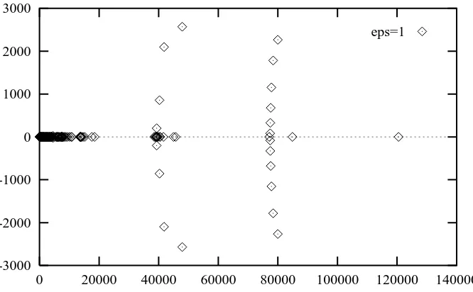
For the construction of an eective iterative solver we now examine the condition number of the spectral operator
L
2; of (1y
R)2(
+au
-3000 -2000 -1000 0 1000 2000 3000
0 20000 40000 60000 80000 100000 120000 140000 eps=1
Figure 10: Eigenvalues of
L
2;SP for N=15, (a,b)=(1,1)
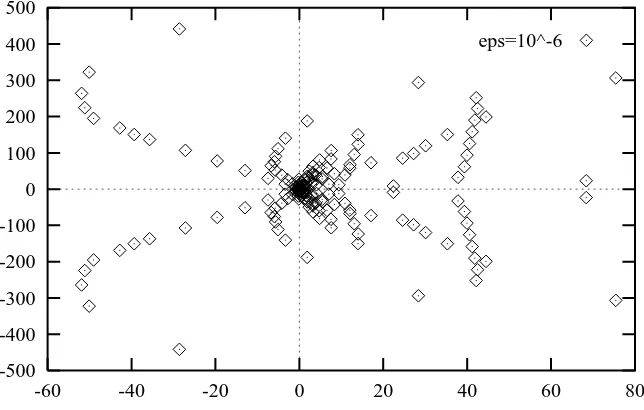
Figures 10 and 11 show the positions of the eigenvalues for
= 1 and= 10 6 for (a,b)=(1,1),N=15.
= 1 = 0(
a;b
)N
max mincond
max mincond
(1
;
1) 3 2:
20102 5
:
91 101 3
:
72 100 8
:
76 100 2
:
43 100 3
:
60 100
7 5
:
71103 5
:
36 101 1
:
06 102 8
:
63 101 7
:
02 101 1
:
23 102
15 1
:
20105 5
:
32 101 2
:
26 103 4
:
43 102 1
:
73 102 2
:
57 103
31 2
:
20106 5
:
30 101 4
:
15 104 1
:
96 103 4
:
24 102 4
:
62 104
( 1
;
1) 3 2:
22102 5
:
82 101 3
:
82 100 3
:
27 100 0
:
00 100
7 5
:
75103 5
:
36 101 1
:
07 102 5
:
03 101 2
:
60 1016 1
:
93 1017
15 1
:
21105 5
:
32 101 2
:
27 103 2
:
86 102 6
:
61 1016 4
:
33 1017
31 2
:
20106 5
:
30 101 4
:
15 104 1
:
29 103 6
:
52 1016 1
:
98 1018
Table 8:
L
2;SPTable 8 gives
max;
min andcond
and demonstrates that there really is an eigenvalue close to0 for (-1,1).
Applying the inverse of the FD operator
L
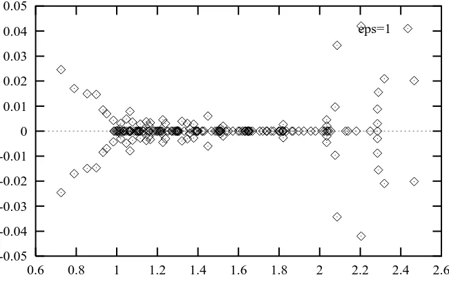
FD as preconditioner, we observe decreased condition number if = 1 while for small , max is unbounded for (1,1). This preconditioner obviouslydoes not stabilize.
Figures 12 and 13 show the positions of the eigenvalues. For small
they are relatively dense positioned with few peak values.In general, FD methods applied to singular disturbance problems are stable if the step size
h
i<
2. Contrary, ifh
i they are unstable. To obtain stability one could increase the [image:12.612.139.472.62.268.2]-500 -400 -300 -200 -100 0 100 200 300 400 500
-60 -40 -20 0 20 40 60 80 eps=10^-6
Figure 11: Eigenvalues of
L
2;SP for N=15, (a,b)=(1,1)
of the upwind method. The rst derivatives @@x and @@y, the convectional part, is discretized by one-sided stream-directed nite dierences while the diusive part is treated with central dierences. We lose one order in convergence but stability is achieved.
We have
a
u
x =a
4
1
y
Ru
xR andb
u
y =b
(2x
R+ 11
y
Ru
xR+ 2u
yR):
According to the factor the derivatives
u
xR andu
yR are discretized by left- or right-dierences in stream direction:u
xR(x
i;y
j)= 8 < :u(xi +1;yj
) u(xi;yj)
xi+1 xi if a 0
u(xi;yj) u(xi 1;yj
)
xi xi 1 if a
<
0for
i
= 0;:::;N
1 ori
= 1;:::;N
. Analogously foru
yR. The upwind method is not uniformly convergent. An adaptive renement might help here. [image:13.612.143.465.64.269.2]-0.05 -0.04 -0.03 -0.02 -0.01 0 0.01 0.02 0.03 0.04 0.05
0.6 0.8 1 1.2 1.4 1.6 1.8 2 2.2 2.4 2.6 eps=1
Figure 12: Eigenvalues of
L
1FD
L
SP for N=15, (a,b)=(1,1)-4000 -3000 -2000 -1000 0 1000 2000 3000 4000
-1000 0 1000 2000 3000 4000 5000 6000 7000 8000 9000 10000 eps=10^-6
Figure 13: Eigenvalues of
L
1 [image:14.612.141.466.96.302.2] [image:14.612.138.469.410.615.2]-1.5 -1 -0.5 0 0.5 1 1.5
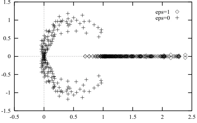
0 0.5 1 1.5 2 2.5
eps=1 eps=0
Figure 14: Eigenvalues of the upstream operator for N=15, (a,b)=(1,1)
-1.5 -1 -0.5 0 0.5 1 1.5
-0.5 0 0.5 1 1.5 2 2.5 eps=1
eps=0
[image:15.612.145.463.131.338.2] [image:15.612.143.469.377.582.2](
a;b
) (1;
1) ( 1;
1)N
max mincond
max mincond
1 3 1
:
40 9:
28101 1
:
51 1:
41 9:
35 101 1
:
507 2
:
06 8:
61101 2
:
39 2:
06 8:
58 101 2
:
4015 2
:
39 6:
99101 3
:
42 2:
39 6:
97 101 3
:
4331 2
:
85 5:
91101 4
:
82 2:
85 5:
91 101 4
:
8210 2 3 6
:
04 101 3
:
04 101 1
:
98 2:
86 101 1
:
11 101 2
:
587 1
:
37 2:
99101 4
:
56 1:
46 2:
67 101 5
:
4915 2
:
18 4:
09101 5
:
34 2:
19 4:
81 101 4
:
5531 2
:
37 4:
34101 5
:
47 2:
37 5:
08 101 4
:
6710 4 3 6
:
66 101 3
:
15 101 2
:
11 3:
33 101 1
:
41 103 2
:
35 102
7 1
:
14 1:
50101 7
:
61 1:
19 3:
10 103 3
:
84 102
15 1
:
29 8:
44102 15
:
3 1:
30 8:
37 103 1
:
56 102
31 1
:
82 8:
08102 22
:
5 1:
82 1:
74 102 1
:
05 102
10 6 3 6
:
67 101 3
:
15 101 2
:
11 3:
33 101 1
:
42 105 2
:
34 104
7 1
:
15 1:
50101 7
:
65 1:
20 3:
11 105 3
:
85 104
15 1
:
31 7:
79102 16
:
8 1:
31 8:
41 105 1
:
55 104
31 1
:
41 5:
72102 24
:
7 1:
34 1:
79 104 7
:
50 103
0 3 6
:
67101 3
:
15 101 2
:
11 3:
33 101 2
:
25 1017 1
:
48 1016
7 1
:
15 1:
50101 7
:
65 1:
20 1:
84 1018 6
:
48 1017
15 1
:
31 7:
78102 16
:
8 1:
31 6:
61 1018 1
:
98 1017
31 1
:
41 5:
69102 24
:
8 1:
34 5:
21 1017 2
:
58 1016
Table 9: Upstream method
It is not satisfactory that there are cases (eg. (-1,1)) in which no stability can be achieved. A possibility to overcome this may lie in the introduction of an additional collocation point. The system is then overdetermined. This method has been examined and successfully applied on the square in [1]. A further method may be the use of staggered grids which possibly leads to
min>
0. Two dierent sets of grids are used - one for the solution and the other one for itsderivative. For the advection-diusion equation there were positive results in [2].
Instead of using the Gauss algorithm for solving the linear systems, one could apply iterative methods. As many other iterative methods do not support complex eigenvalues we recommend the use of the GMRES method (see [5]) - a method of minimized residuals. The linear system
Bv
=g
whereB
is a non-symmetric and large matrix is solved as follows.v
0is the initial solution,r
0 =g Bv
0 and we dene the m-th Krylov spaceK
m:=span
fr
0
;Br
0;:::;B
m 1
r
0g. Then we
nd the approximation
v
m 2v
0+
K
m such that the m-th residualr
m fulllsj
r
mj=min
!.Domain decomposition
consider the Poisson equation with Dirichlet boundary condition
u
=f
in;
u
=g
on@
:
At the interface between two subdomains, information is exchanged until continuity is reached. In one direction Dirichlet information is transfered and in the other direction it is Neumann information. We use an interface relaxation as proposed in [3] i.e. at the Dirichlet side we hand over a weighted sum of subsolutions at the interface. We iterate until the error at the interface is smaller than 10 14. Thus we iteratively solve a sequence of Dirichlet Neumann problems. We
begin with a domain composed of one patched triangle and square =
T
[R
whileT
= f(x;y
) j0< x;y <
1 andx
+y <
1g andR
= f(x;y
) j0< x <
1 and 1< y <
0g:
6
-@ @ @ @ @
x
y
1
-1 -1
1
R T
Figure 16: Domain
The interface is = (0
;
1)f0g (Figure 16). Initial conditions areu
0 1 =u
0 2
0 on and
u
11 =
g
on . We then iterateu
m1 =
f
inT;
u
m1 =
g
on@T
n;
u
m1 =
m 1
u
m 12 + (1
m 1)
u
m 1 1 onand
u
m2 =
f
inR;
u
m2 =
g
on@R
n;
@
@yu
m2 =@
@yu
m1 on:
Here
m denotes the relaxation parameter which is chosen dynamically. This dynamical choiceusually accelerates the convergence.
m =is the unique number which minimizesk
z
m()z
m 1() k2
2 where
z
m() =u
m
2 + (1
)u
m
1 .
m is calculated by
m = (e
m1;e
m
1
e
m
2 ) k
e
m1
e
m
2 k
2 2
where (
:;:
) denotes the discrete L2 inner product ande
mi=u
miu
m 1i for
i
= 1;
2is the dierence of two consecutive iterates on the two subdomains.
m should be in (0;
1].We cannot use example (1) because this function vanishes at the interface. Therefore no new information is exchanged which makes an iterative method superuous, as it converges after the rst step. Thus we introduce the following oscillating example
u
(x;y
) = sin(x
)sin(y
+4):
(2)N It
E
2TE
2R4 15 1
:
36102 1
:
28 102
8 17 2
:
42105 1
:
64 105
16 17 8
:
011013 4
:
24 1013
32 17 1
:
001014 1
:
60 1014
Table 10: with (2)
Table 10 shows the number of iterations and the discrete L2 error on square and triangle. We
reach the tolerance after relatively few steps. The convergence is fairly slow because of the oscillatory behaviour of the solution. The number of iterations is constant and independent of N. Machine accuracy is reached for N=16.
The second domain 1 to be studied consists of and an additional triangle
T
1 attached to thealready existing one (Figure 17).
6
-@ @ @ @ @
x
y
1
-1 -1
1
R T T1
Figure 17: Domain 1
We begin with triangle
T
with interface boundaries 1 = (0;
1)f0g and 2 =
f0g(0
;
1) and= 1 [
2. Then we solve on
R
andT
1. This should be realized on a parallel computer. The [image:18.612.228.378.425.588.2]u
m1 =
g
on@T
n;
u
m1 =
m 1 1
u
m 1
2 + (1
m 1 1 )
u
m 1 1 on
1
;
u
m1 =
m 1 2
u
m 1
3 + (1
m 1 2 )
u
m 1 1 on
2
;
and
u
m2 =
f
inR;
u
m2 =
g
on@R
n1
;
@
@yu
m2 =@
@yu
m1 on 1;
and
u
m3 =
f
inT
1;
u
m3 =
g
on@T
1n 2
;
@
@xu
m3 =@
@xu
m1 on 2:
N It
E
2TE
2RE
2T14 65 1
:
04102 9
:
62 103 1
:
25 102
8 83 6
:
98106 5
:
67 106 2
:
68 105
16 84 6
:
851013 4
:
01 1013 1
:
02 1012
32 90 2
:
311013 8
:
30 1014 9
:
90 1014
Table 11:
1 with (3)
Initial values are analogous to the last example. We apply this algorithm to the example
u
(x;y
) = sin(x
+4)sin(y
+ 4):
(3)The results are listed in Table 11. The number of iterations is extremely increased if a further triangle is added. Unfortunately,
mi tends to leave the interval (0;
1]. Whenever this happens, the following approximation is worse than the one before. Nevertheless, the method nally converges. This dynamical choice ofmi is not optimal. We have derived results for xedmi = 12
in Table 12.
N It
E
2TE
2RE
2T14 34 4
:
89104 2
:
82 104 1
:
51 103
8 41 9
:
29109 2
:
30 109 6
:
82 108
16 46 1
:
781013 3
:
70 1014 1
:
83 1013
32 87 9
:
681013 8
:
40 1014 1
:
01 1012
Table 12:
1 with (3) and
m = 0
:
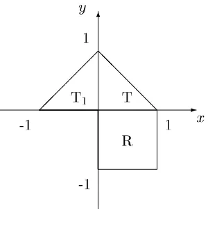
5Finally, we study the domain 2 =
R
[T
1 [
T
2 [
T
3 [
T
4 (
T
i triangles) which is symmetric tothe origin (Figure 18). We consider the following example
u
(x;y
) = sin(3x
+4)sin(3y
+4):
(4)6
-@
@ @ @ @
@ @
@ @
@
x
y
1
-1 -1
1
Figure 18: 'wind wheel' 2
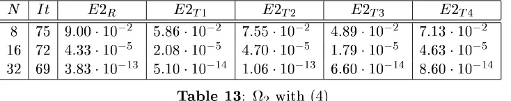
The algorithm is analogous to the last one and we rst solve on the square and then on the triangles. The results in Table 13 are fairly good for symmetry reasons considered that we now deal with ve subdomains. The number of iterations is constant and machine accuracy is reached for N=16.
N It
E
2RE
2T1E
2T2E
2T3E
2T48 75 9
:
00102 5
:
86 102 7
:
55 102 4
:
89 102 7
:
13 102
16 72 4
:
33105 2
:
08 105 4
:
70 105 1
:
79 105 4
:
63 105
32 69 3
:
831013 5
:
10 1014 1
:
06 1013 6
:
60 1014 8
:
60 1014
Table 13:
2 with (4)
[image:20.612.89.419.80.301.2] [image:20.612.119.486.401.474.2][1] H.Eisen, W. Heinrichs, A new method of stabilization for singular perturbation
prob-lems with spectral methods. SIAM J. Numer. Anal. 29, pp. 107-122 (1992).
[2] D. Funaro, A fast solver for elliptic boundary-value problems in the square. Comput.
Methods Appl. Engrg. 116, pp. 253-255 (1994).
[3] D. Funaro, A. Quarteroni, P. Zanolli, An iterative procedure with interface
relax-ation for domain decomposition methods, SIAM J. Num. Anal., 25, pp. 1213-1236 (1988) [4] M. Griebel, T. Dornseifer, T. Neunhoeffer Numerische Simulation in der
Stromungsmechanik. Vieweg Lehrbuch, 1995.
[5] W. Heinrichs, Defect correction for convection-dominated ow. SIAM J. Sci. Comput.,
17, No. 5, pp. 1082-1091, 1996.
[6] W. Heinrichs, Spectral collocation on triangular elements, J. Comp. Ph., 145, pp.
743-757 (1998)
[7] S. Sherwin, G. Karniadakis, Triangular and tetrahedral spectral elements.