Non-steady time series analysis in the developing embryo

Rochester Institute of Technology

RIT Scholar Works

Theses

Thesis/Dissertation Collections

11-21-1995

Non-steady time series analysis in the developing

embryo

Daniel Kettles

Follow this and additional works at:

http://scholarworks.rit.edu/theses

This Thesis is brought to you for free and open access by the Thesis/Dissertation Collections at RIT Scholar Works. It has been accepted for inclusion

in Theses by an authorized administrator of RIT Scholar Works. For more information, please contact

[email protected].

Recommended Citation

NON-STEADY TIME SERIES ANALYSIS IN

THE DEVELOPING 'EMBRYO

A Thesis Submitted in Partial Fulfillment of the Requirements for the

Masters of Science Degree in Mechanical Engineering

at Rochester Institute of Technology

on November 21, 1995

By

Daniel E. Kettles

Approvals:

Dr. Charlie Haines, Department Head

Dr. Mark H. Kempski, Thesis Advisor

Dr. Kevin Kochersberger, Thesis Committee

Release

I, Daniel

E.

Kettles, do hereby give permission to Wallace

Memorial Library to reproduce this Thesis, entitled

Non-Steady Time

Series Analysis in the Developing Embryo,

in

whole or

in

part. Any such

reproductions may not be for commercial use or profit.

Signed,

Daniel

E.

Kettles

Acknowl

edgments

To

recognize all of

the

people who

helped,

influenced

or encouraged me

in

some

way

while

I

was

working

on

this

thesis

would

be nearly

impossible.

However. I

would

like

to

thank the

following

people who come

to

mind.

My

parents,

Frank

and

Cynthia

Kettles,

along

the

rest of

my

family

at

105

Green Clover Drive for

their

emotional

support;

My

graduate

advisor,

Dr. Mark

Kempski,

for his

support and

encouragement;

Dr. Edward Salem

and

Dr. Kevin

Kochersberger,

for accepting my

invitation

to

be

on

my

thesis committee,

and

for

agreeing

to

review

my

thesis

so close

to

final

exams and

the

end-of-quarter

rush;

Shri,

Mike,

Andrew

and everyone else at

the

Biosystems Lab

(including

the

students who used

the

lab

as a

hangout!)

for

their

encouragement and

assistance;

Table

of

Contents

Table

of

Contents

i

List

of

Figures

iii

Abstract

viii

1.

Introduction

1

1

.

1

Hemodynamics

of

the

Embryonic

/

Fetal

Cardiovascular System

1

1.2

Justification

for Research

6

1.3

Research

Goals

7

2.

Methodology

10

2.1

Methods Employed

in

Previous Work

10

2.2

Relationship

to

Other Research

13

2.3

Removing

Spurious Data

16

2.4

Grouping

Embryo Spectra

24

2.5

Band Power

Determination

28

3.

Results

42

3. 1

Frequency

Domain Effects

of

Data Removal

42

3.2

Grouped

Embryonic

Data

50

3.2.1

Algorithm Validation

with

Test Data

50

3.2.2

Sample Results

with

Chick Data

52

3.3

Spectral

Band

Power

58

3.3.1

Algorithm

Validation

with

Test

Data

58

3.3.2

Sample Results

with

Chick Embryo Data

61

3.4

Joint

Time-Frequency

Analysis

3.4.1

Algorithm Validation

with

Test

Data

70

3.4.2

Spectrograms

with

Chick Embryo Data

72

4.

Discussion & Conclusions

79

4.1

Discussion

of

Results

79

4.2

Future Lines

of

Research

82

References

86

Appendix

A

Discrete Spectral

Analysis

89

A.l

The Discrete

Fourier

Transform

(DFT)

89

A.2

The

Fast

Fourier

Transform

(FFT)

92

A.3

Spectral

Representations

and

Power

93

A.4

Zero

Padding

98

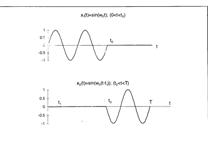
Appendix B

Special Case in

Spectral

Analysis-Frequency

Domain

Analysis

of

Sectioned Sinusoids

107

Appendix C Algorithm Usage &

Programming

Overview

114

C.l

Edit

and concatenate.vi

114

C.2

Linear interpolation Il.vi

120

C.3

Band

power calculation

(5 bands).vi

Band

powercalculation

(10 bands).

vi

127

C.4

Short

time FFTl.vi

130

Appendix D MATLAB Routines

D.l

Spectra.m

137

List

of

Figures

Figure

Description

Page

Section

1

1-1

Transformation

of

the

heart

tube

into

the

mature

four

chambered

heart.

2

1-2

Schematic

of

the

cardiovascular control mechanisms

responsible

for

heart

rate

variability

in

the

mature

heart.

4

Section

2

2-1

Interrelationship

between

algorithms used

in

this

work and

previously defined

algorithms.

14

2-2

Derivation

of cardiovascular

variability

time

series.

15

2-3

Corrupted human fetal blood

velocity

data.

17

2-4

(a)

Blood

velocity

time

series with corruption

for 'tail

to

head'

concatenation example.

(b)

Results

of

'tail

to

head'concatenation.

19

2-5

(a)

Schematic

of

threshold

crossing

concatenation method.

(b)

Resulting

velocity

time

series after

threshold

crossing

concatenation.

21

2-6

Concatenated

velocity

data from Figure 2-5

with subsequent

scaling.

23

2-7

Typical

result of

interpolating

and

averaging

two

embryospectra.

28

2-8

'Chirp'

data

used

for

JTFA

example.

33

2-9

Discrete PSD

of

the

chirp'

signal

from Figure

2-8.

34

2-10

Three

dimensional

time-frequency

analysisrepresentationof a

'chirp'

Figure

Description

Page

2-11

Basic

procedure

for

short

time

Fourier

transform.

37

2-12

Block

diagram

of

moving

overlapped windows on a

data

set.

39

Section 3

3-1

Sinusoid

with section removed as an example of

sectioning

out

data from

a

sinusoidally varying data

set.

44

3-2

Superimposed

amplitude spectra

for

the

original and altered

sinusoids

in

Figure 3-1.

45

3-3

Three

dimensional

amplitude spectrumrepresentationof a

sinusoid with an

incrementally increasing

section removed

from

the

middle.

47

3-4

(a)

Interpolated

peak

velocity variability

PSD

for

two

Stage

14

embryos.

(b)

Average

PSD.

54

3-5

(a)

Interpolated

peak

velocity variability

PSD

for

two

Stage

27

embryos.

(b)

Average PSD.

55

3-6

(a)

Interpolated heart

rate

variability

PSD

for

two

Stage

14

embryos.

(b)

Average PSD.

56

3-7

(a)

Interpolated

HRV PSD for

two

Stage

27

embryos.

(b)

Average PSD.

57

3-8

PSD

of

the

sequence given

by

eq.

(3.1)

in

arbitrary

units.

60

3-9

Stage 14

peak

velocity

variability

spectral

band

power.

63

3-10

Stage 27

peak

velocity variability

spectral

band

power.

63

Figure

Description

Page

3-12

Stage

27 HRV

spectral

band

power.

64

3-13

Stage

14

peak

velocity variability

spectral power

distribution.

66

3-14

Stage

27

peak

velocity variability

spectral power

distribution.

66

3-15

Stage 14 HRV

spectral power

distribution.

67

3-16

Stage

27 HRV

spectral power

distribution.

67

3-17

Stage

14

HRV

spectral power

distribution

with

10

.25

Hz

wide

frequency

bands.

69

3-18

Stage 27 HRV

spectral power

distribution

with.25

Hz

frequency

bands.

69

3-19

Spectrogram

of

test

data

series

in

eq.

(3.4).

72

3-20

(a)

Stage 14

chick embryo

blood velocity data

segment.

(b)

Spectrogram

of

Stage

14

chick embryo

blood

velocity

time

series

data.

74

3-21

(a)

Stage

14

chickembryo peak

blood

velocity variability

time

series

data.

(b)

Spectrogram

of

Stage

14

peak

velocity

variability

time

series.

75

3-22

Peak

velocity

variability

spectrogram with

1024

point window

length

and

256

point

increment.

77

Appendix

A

A-l

The

frequency

domain

effects of

sampling

an

analog

signal.

91

A-2

Sample

discrete

PSD

showing

the

development

of

integration

Figure

Description

Page

A-3

(a)

Discrete

PSD

of

Chirp

data

without zero padding.

(b)

Discrete PSD

of zero padded 'chirp'

data

withoutzero

padding

correction.

(c)

Discrete PSD

of zero padded

'chirp'

data

withzero

padding

correction.

101

A-4

Superimposed

Harming

and rectangular windows.

104

A-5

Sinusoid from

eq.

(A.15)

with a

Hanning

window applied.

105

A-6

PSD

(log

magnitude

form)

of sinusoid with and without

Hanning

window applied.

105

Appendix B

B-l

Sinusoid

withsection removed.

108

B-2

Individual

sinusoids

that

sum

to

form

a sectioned sinusoid

Abstract

Cardiovascular diseases

with origins

in

early fetal

development

are a

serious

health

concern

in

the

United States.

Presently,

there

are

few,

if

any,

diagnostic

tools

available

for doctors

to

determine

the

overall

health

of

the

early

fetal

cardiovascular system

in

a non-invasive manner.

This

thesis

is

a

step

toward

the

development

of a non-invasive system

for

the

detection

ofcardiovascular

malformations

in

the

early human

fetus. The

computeralgorithms presented

in

this

work

dovetail

with other algorithms

to

represent embryonic

/fetal

cardiovascular output and

variability

data

in

the

frequency

domain. Algorithms

in

this thesis

allow

the

capability

to

editexternal artifact

from

data,

determine

common

frequency

spectra

forms

and calculate spectral

band

power

to

aid

in

study group

comparison.

Additionally,

an algorithm

is

presented

to

represent

1.

Introduction

Congenital

cardiovascular malformations are a serious

health

concern

in

the

United

States

(Clark

and

Takao 1990). At

present

there

are no clinical

tools

to

asses

the

health

of

the

early

embryonic

/fetal

cardiovascularsystem.

However,

it

has been hypothesized

that

beat

to

beat variability

in

embryonic

/fetal heart

rate

and

blood velocity

correlate

directly

to

cardiovascular well

being

(van

Ravenswaaij-Arts

1993,

Breborowicz

1988,

Kempski 1995).

This

thesis

is

a

step

toward the

development

of a non-invasive

technique

for assessing

the

cardiovascular

health

of

the

10

to

18

week

human fetus.

Early

detection

of abnormal

fetal

cardiovascular output can

lead

to

more effective

treatment

protocols

early

in

gestation.

This

section

begins

with an overview of

the

development

and

hemodynamics

of

the

embryonic cardiovascular system.

Later,

an overview of

congenital cardiovascularmalformations

is

presented as a

justification

for

the

research.

This

section concludes with a

summary

of previous work

(Gallagher

1995)

which

directly

impacts

the

scope and objectives of

this thesis.

1.1 Hemodynamics

of

the

Fetal

Cardiovascular System

The

cardiovascularsystem

is

the

first

functioning

organ

in

the

embryo/fetus.

Through

a complexprocess

known

as

morphogenisis, the

to

a

four

chambered

heart.

In

the

human

fetus,

the

musclewrapped

heart

tube

begins

beating during

the

third

gestational week.

For

the

next

three to

four

weeks,

mechanical

forces

related

to

function,

morphogenisis and growth

transform

the

heart

tube

into

the

mature

four

chambered

heart (Clark

and

Van

Mierop

1989,

Marieb

1992)

(Figure

1-1). Few

majorstructuralchangesoccur

in

the

heart

during

mid

to

late

gestation.

Superiorvenacava Right pulmonary artery Pulmonarytrunk Right Atrium Right pulmonaryveins Fossa ovalis Pectinate. muscles Tricuspid valve Bightventricle Chordae tendineae Trabecuiae carneae Inferior vena cava Aorta Leftpulmonary artery Lettatrium Lett_pulmonary veins Pulmonary semilunarvalve Bicuspid (mitral)valve Aortic semilunarvalve Leftventricle Papillary muscle Interventricular septum Myocardium Visceral pericardium

Figure 1-1.

Transformation

of

the

heart

tube

into

the

mature

four

chambered

The early

embryo

/fetal

cardiovascular

system,

like

that

of

the

mature

system,

is

regulated

to

meet

demand

(Kempski 1993

and

1995,

Clark

1990).

Unlike

the

mature

system,

however,

variations

in

embryo/fetalcardiac output

early

in

development

are not regulated

by

the

central nervoussystem.

Autonomic

cardiovascular control

in

the

chick embryo

does

not

begin

until after

Stage

271

(Pappano

1977,

Sissman 1970).

Thus,

the

early

cardiovascularsystem

distributes

oxygen andnutrients

to

the

growing

embryo without

the

sophisticated regulation mechanisms present

in

the

mature system.

The

mature cardiovascular

system,

in

contrast,

is

regulated

by

a complex

feedback

control system

(Figure

1-2). Beat

to

beat

pacing

is

controlled

by

sympathetic and

parasympathetic2 nervous system

activity

and

feedback

occurs

through

respiratory

sinus

arrhythmia3,

baroreflex"

and

thermoregulation

(Marieb

1992,

van

Ravenswaaij-Arts

1993,

Kempski

1995,

Saul

1991).

1

'Stage27'

is from

the Hamburger-Hiltonscale

for

measuring

chick embryo

development. Stage

27 is approximately 51/2 days

ofgestation,and correlatestoabout

37

days

of

human fetal

gestation(Sissman 1970). 2

The

sympatheticnervous system causes

heart

rateto

increase in

responsetocrisis situationsand exercise.

The

parasympathetic nervous system counterstheaffectsofthesympatheticnervous system oncethecrisis situation or exercise

has

passed.

3

Respiratory

sinusarrhythmiaisa phenomenathatrelatesthe

frequency

of

heart

rate

variability

to the

breathing

rate.

4

Vagus

SANode

ILVtt) respiration

K

Sjrnnparetics

LPF

0 Hz 05

LPF

0 Hz 05

t

hea-t

htt)

A

ventricles

and vasculature

bar

preceptors

arterial pressure

ABPCt)

respiration ILVtt)

*dt

Figure

1-2.

Schematic

of

the

cardiovascular control mechanisms responsible

for

heart

rate

variability

in

the

mature

heart.

Redrawn

from Saul

1991.

Less is known

about

the

exact mechanisms of

fetal

cardiac control and

normalcardiac output

early

in

gestation

than

in

the

mature system.

However,

research on

White

Leghorn

chick embryos

(Kempski

1993,

Hu

and

Clark

1989)

and

sheep

embryos

(Adamson

1992)

has

indicated

that

four determinants

of

myocardial contractility.

These four

determinants

are also present

in

the

mature

cardiovascular system

(Clark 1990).

Preload is

determined

by

diastolic,

orventricular

filling

events.

Changes

in

preload occur

in

response

to

environmental and metabolic

demands

in

the

embryo.

The

Frank-Starling

Law

of

the

Heart,

which

describes

the

biomechanical

properties of

stretching heart

muscle,

is

a

beat

to

beat

regulation phenomenon.

According

to the

Frank-Starling

Law

of

the

Heart,

stroke work

is

controlled

by

the

amount of preload on

the

cardiac muscle cells

just

before

they

contract.

More

details

on

this

process can

be

found

in

ref.

(Marieb

1992).

Afterload

refers

to the

impedance

of

the

vascular

bed. Vascular

impedance is

due

to

a combination of resistance

to

flow,

fluidic

capacitance,

blood

inertance,

varying

blood

vessel wall

tension

and vessel caliber.

In

the

chick

embryo,

vascular

impedance is

also

influenced

by

temperature.

In

addition,

neurohumeral

agents5

present

in

the

blood

stream of

the

early

chick embryo

(2

to

6 days

of a

21

day

gestation)

are speculated

to

provide some

hemodynamic

regulationrelated

to

afterload

(Hu

and

Clark

1989,

Clark

1990,

Nakazawa

1989).

Heart

rate

in

the

chickembryo

is

temperature sensitive,

or poikilothermic

in

nature.

It

has

been

shown

that

as embryonic

temperature

increases,

the

heart

rate

(and

cardiac

output)

increases,

while as

the

embryo

cools,

the

heart

rate

5

Neurohumeralagents are chemicals present at nerve endingsthatexcite adjacentstructures,

decreases.

Embryo

temperature

also

has

an

inverse

relationship

to

afterload

(Nakazawa

1985). The

heart

rate of

the

human

fetus, however,

is

regulated

by

hypoxia

and

hyper

capnict

\

Myocardial

contractility

can

be

shown

through

the use of

the

pressure-volume

loop,

which relates

instantaneous

ventricular pressure

to

volume

(Clark

1990). The

total

area enclosed within

the

pressure volume

loop

is

a measure of

the

amount of myocardial work

(Suga

1979).

1.2

Justification

for Research

Cardiovascular

malformations are a serious

health

problem

in

the

United

States.

Specifically,

for every

1000

births,

8

to

10 infants

have

some

kind

of congenital cardiovascular

defect (Clark

1990).

In

many

cases, the

defect

can

be

corrected with post natal surgery.

However,

20%

of all

infants

with

cardiovascular malformations will

die before

their

first

birthday

regardless of

heroic

surgical

intervention.

Examples

of cardiovascularmalformations

include

myocardial

(heart

muscle)

defects,

valve

defects

and

tetrology

of

Fallot7. Despite

advanced surgical

techniques

to

correct

many fetal

cardiovascular

defects,

there

is

still a

lingering

morbidity

that

limits

the

life expectancy

of

many

children and adults with congenital

heart

defects. In

addition,

some adult cardiovascular

6

Hypoxia

refersto

low blood

oxygen

levels. Hypercapnia

refersto

high blood

carbon

dioxide

levels.

7

Tetrology

of

Fallot is

a serious

heart defect

involving

many

conditions,

including

constrictionof

diseases,

such as

coronary artery

disease

and

hypertension

may have

their

origins

early

in

cardiac

development

(Clark

1990).

1.3

Research Goals

The

long

term

goals of research related

to this thesis

are

to

correlate

beat

to

beat

and

long

term

variability

in

embryonic

/fetal

cardiovascular output

to

cardiovascular well

being.

To

accomplish

this,

a control system approach will

be

used

to

analyze

variability

in

fetal

cardiovascular

output,

similar

to that

shown

in

Figure

1-2.

The

computer algorithms presented

in

this thesis

dovetail

with

others

(Gallagher

1995),

and will

be

used

to

quantify

'normal' and

'abnormal'

fetal

heart

rate and

blood

velocity

variability.

Using

results generated

from

the

algorithms presented

in

this thesis

and

others

(Gallagher

1995),

temperature

regulation

in

chick

heart

rate

variability

can

be

investigated.

For

the

human

fetus,

cardiovascular control mechanisms which

affect

heart

rate

variability

can

be

scrutinized.

In

addition,

analysis of peak and

meanpulsatile

blood

velocity variability

can

be

used

to

identify

other

cardiovascularcontrolmechanisms such as vascular

impedance.

Use

of

human

data. The

algorithms presented

in this thesis

will

be

used

to

analyze cardiovascular

data from both

chick embryos and

human fetuses.

It is

very

important

to

note

here

that

human fetal

cardiovascular

data

is

obtained

granted

before any fetal data

is

acquired and analyzed.

In

addition,

data from

other

subjects,

such asadultsandneonates

may be

analyzed

in

the

future

using

these algorithms,

subject

to

full

consent.

The

algorithms

described herein

serve

to

supplementsoftware algorithms

whichacquireandreconstruct

Doppler

velocity

waveforms.

In

addition, the

currentalgorithmsseek

to

extend

the

data

analysis capabilities when

performing

power spectral analysis on

blood velocity

and

heart

rate

variability

waveforms.

Due

to

such

factors

as

variability

amongst embryonic/fetal

study

groups,

spurious

inputs

due

to

movement artifact or

the

non-steady

nature of

cardiovascular

time series,

additional

post-processing

is

implemented

using

the

algorithms presented

here.

Thus,

the

specific goals of

this thesis

are:

To

present an algorithm

to

'edit'spurious

data from

a

blood

velocity

time

series.

The

spurious

data

may be

present

due

to

embryo

/fetus

movement,

maternal movement or

instrumentation

noise.

This

algorithm

is

to

be

used on

reconstructed

velocity

time

series

before any

analysis

is

implemented.

To

compensate

for

variability

among

embryos/fetuses

in

a particular

study

group

and

differences

in

data

record

lengths,

an algorithm

is

presented

to

interpolate

groups of spectral

data

sets

to

a common

frequency

axis.

Quite

often

in

spectral

analysis,

it is

desirable

to

calculate

the

amountof

spectral

'power'

Dominant

frequency

bands

can

be

therefore

determined for heart

rate and

blood velocity

variability

in

the

embryo

/fetus.

Thus,

an algorithm

is

presented

to

calculate

the

amount of'power'contained within specific

frequency

bands

of

the

PSD

data.

Cardiovascular

output

is

non-steady

in

nature.

In

other

words, the

regulatory

mechanisms

(afterload,

blood

oxygenation,

chick embryo

temperature

etc.)

cause

the

component

frequencies

of

blood velocity variability

and

heart

rate

variability

to

vary

over

time.

Spectral

analyses of a

data

set

taken

in

toto

cannot

describe

how

orwhen

the

frequencies

change.

Thus,

an algorithm

is

presented

to

show

the time-dependent

spectral content of cardiovascular

variability

data.

The

methodologies

behind

these

goals are presented

in

the next section.

2.

Methodology

In

order

to

correlate variations

in

cardiovascular output with

cardiovascular control

mechanisms,

mathematical methods

that

accurately

quantify

these

variations are needed.

Recall

from

the

previous section

that

variations

in

heart

rate and

blood velocity may be linked

to

hemodynamic

control mechanisms

in

the

embryo

/fetus. The

control mechanisms are

influenced

by

afterload, thermoregulation

(in

the

chick

embryo)

and oxygenregulation

(in

the

human fetus).

The

analysis of

the

cardiovascular output

variations,

either

in

the

time

domain

or

the

frequency

domain,

can

help

explain and

quantify

the

biological

mechanisms

for

embryonic

/fetal

cardiovascular control.

In

this section,

an overview of

the

methodologies

that

are utilized

in

this

thesis

is

presented.

Theories behind

these methods,

along

with

the

applicable

mathematical

derivations

arepresented

in

Appendices A

and

B.

Programming

and usage

details

for

the

software algorithmspresented

in

this thesis

are given

in

Appendices

C

and

D.

2.1

Methods

Employed

in Previous Work

Much

work

has

been

done

to

quantify

the

variability

of cardiovascular

signals,

particularly

with

heart

rate

variability

in the

adult and

infant.

Two basic

time

domain

analysis

(van

Ravenswaaij-Arts

1993,

Parer

1985,

Yana

1993)

and

frequency

domain

(spectral)

analysis

(van

Ravenswaaij-Arts

1993,

Kempski

1993,

Saul

1991,

Akselrod

1985,

Breborowicz

1988,

Kuo

1993,

Adamson

1992,

Goldstein 1993

and

1994)

Time

domain

methods.

There

are a number of

different

methods

available

to

analyze cardiovascular signals

in

the time

domain.

One

approach

involves

the

calculation of

short-and long-

term

indices

directly

from

the time

series representation of

the

cardiovascular signal

(van

Ravenswaaij-Arts

1993,

Parer

1985).

Short

term

variability

involves

the

changes of

the

cardiovascular

signal on a

beat

to

beat basis.

Long

term

variability

seems

to

have different

interpretations

depending

on

the study,

but

can

be

thought

of as a

longer-duration

change

in

heart

rate

(i.e.,

over severalcardiovascular cycles).

One form

of

the

short- _andlong-

term

indices involves

_{the standard}

deviation

from

the

mean

heart

rate.

Others involve

such methods as modification

of

the mean,

sorting

and

selecting,

and calculations ofslope changes. Short- and

long-

term

index

methods

have

been

shown

to

be computationally

inexpensive

ways

to

categorize short

term

heart

rate variability.

However,

only

one of nine

indices

validly

measured

long

term

variability

(Parer 1985).

Since

the

range of

frequencies below 1

Hz1

(Kempski

1993,

Akselrod

1985,

Breborowicz

1988,

1

Goldstein 1993

and

1994)

is

of

primary

interest

in

evaluating

cardiovascular

fluctuations,

the

determination

of

variability

in

the

sub-heartrate range

may be

problematic

using

the

above methods.

There

are other methods available

for analyzing

cardiovascularsignals

in

the

time

domain. Autocorrelation

is

essentially

the

time

domain

comparison of a

delayed

version of a signal

to

itself,

and

is

equal

to the

inverse

Fourier

transform

of a

Power

Spectral

Density

(PSD)

representation of

the

signal

(Stremler

1990).

The

subsequent

Fourier

transform

of

the

autocorrelation

function

yields

the

PSD

of

the

signal.

Autocorrelation

is

used

in

applicationswhere

the

signals

to

be

analyzed are corrupted

by

noise

(Stremler

1990). A

possible

drawback

to

autocorrelation,

however,

is

that

it

adds a second

step

(in

the time

domain)

to the

computation of the

frequency

domain

representation of a signal.

Frequency

domain

(spectral)

analysis.

Using

spectral

analysis, the

variations of

heart

rate and peak

blood

velocity

can

be

represented

by

their

frequency

components.

The

Fourier

transform

is

the

basis

for

frequency

domain

analysis

(see

Appendix

A). In

essence,

frequency

domain

methodologies

involve

the

decomposition

of periodic or aperiodic signals

into

a summation of sine

waves at

different frequencies. For digital

computer

implementation,

the

Fast

Fourier

Transform

(FFT)

algorithm

is

primarily

used.

Thanks

to the

advent of

become very

popular

in

signal

processing

applications,

including

cardiovascular

signals

(van Ravenswaaij-Arts

1993).

The

above

time

and

frequency

domain

methods allow

the

quantification

of cardiovascularoutputas

it

varieswith

time.

Methods

have

also

been

developed

to

correlatecardiovascularoutput

(in

adult

humans

and

dogs)

to

control system

models,

including

system

impulse

response

(Yana

1993)

and

transfer

functions

(Saul 1991). Similar

methods can

be

used

in

future

research

to

develop

control parameters

for

the

fetal

cardiovascular system.

2.2

Relationship

to

Other Research

The human

fetal

blood

velocity

data

used within

this thesis

is

provided

by

Dr.

Juriy

W. Wladimiroff (and

colleagues)

of

Academic

University

Hospital

in

Rotterdam,

The

Netherlands.

The

chickembryo

data,

which was used as 'pilot'

data for

algorithm

development,

wasprovided

by

Mr. Norman Hu

of

the

University

of

Rochester

and

Dr. Monique L. Broekhuizen

of

Academic

University

Hospital,

Rotterdam.

The

algorithms

developed for

this thesis

are used

in

concert with others

developed

by

Francis J. Gallagher (1995).

All

custom analysis algorithms

for

this

thesiswere

developed

using

Lab

VIEW2

graphical

programming

software

for

instrumentation

(see

the

end of

this

section

for

a

listing

of

these

algorithms).

A

flow

chart

showing

the

interrelationship

between

the algorithms

is

shown

in

1

Figure

2-1

on

the

next page.

The

algorithmsshown

in

gray boxes

involve the

derivation,

spectralanalysisand normalization of

the

cardiovascular

time

series.

They

are

detailed further

in

(Gallagher,

1995).

Velocity

Time

Series

Reconstruction

From Video Tape

From

Data File

i

Edit Spurious

Information from

Velocity

Data

+

Generate

Variability

Waveforms

1 I

Peak Amplitude

Variability

Heart

Rate

Variability

i

PSD

Analysis

on

individual

Embryos

Normalized

Non-Normalized

*

Interpolate

PSDs

to a

Common

Frequency

Axis

i

Band Power

Calculations

-?

Joint

Time-Frequency

Analysis

1

JTFA Spectragram

Time Variable Band Power

Leqend:

=

Previously

generated algorithms

(Gallag

her,

1995)

Figure 2-1.

Interrelationship

between

algorithms used

in

this

work and

Cardiovascular

variability

time

series

(Gallagher,

1995).

Two

forms

of

cardiovascular

variability data

are of

interest

for

spectral analysis

(see

Figure

2-2). Instantaneous Heart Rate

and

Heart Rate

Variability

are obtained

from

the

beat

to

beat periodicity

(AT;)

at a threshold crossing.

The

threshold

crossing

is

equal

to

the

global mean

blood

velocity.

The beat

to

beat periodicity is

inverted

(1/AT;)

to

obtain

the

instantaneous heart

rate.

Heart

rate

variability

is

obtained

by

subtracting

the

global mean

heart

rate

from

the

instantaneous

heart

rate.

Peak

velocity variability

(AVpi)

represents

the

beat

to

beat difference between

adjacent

amplitudes.

The derivations

of

instantaneous heart

rate and peak

velocity

variability

are

diagrammed

in

Figure

2-2.

o v (A

u o

>

Blood

Velocity

Profile (13 Week Human

Fetus)

Threshold

1

Av

T

AT,

Time

(sec.)

Figure

2-2. Derivation

of cardiovascular

variability

time

series.

The FFT

of

the time

series

data is

converted

to

the

Power

Spectral

Density

(mm/sec)2/Hz for

peak

velocity variability

spectra.

The

frequency

axis

is in Hz

(cycles/second).

Therefore,

the

PSD

spectrum can

be

thought

of as a

distribution

of signal spectral power per unit

frequency.

Normalization

of spectra.

Because different

embryos

/fetuses

at a given

gestational age

may have different

mean

heart

rates and mean

blood

velocities,

normalization of

the

spectral

(PSD)

representations

is

performed.

PSDs

of peak

velocity variability

data

are normalized

by

thesquare of

the

cardiac cycle mean

velocity

of

the

respective

data

series.

PSDs

of

threshold

crossing

heart

rate

variability

are normalized

by

the square of

the

mean

heart

rate

determined from

the

data

series.

The

frequency

axes of all normalized

PSDs

are

divided

by

the

mean

heart

rate

(in

Hz)

determined from

the

original

velocity

time

series

data.

Normalized PSD

spectra

have

units of

1/Hz,

with unitless

frequency

axes.

The

normalized

PSDs

are used

for

relative comparisons

between different

embryos

/fetuses.

The

algorithms can also generate non-normalized spectra

(i.e.,

absolute

PSD data).

2.3

Removing

Spurious Data

Fetal blood

velocity

data

can get corrupted

by

fetal

or maternal

movement,

or

by

instrumentation

noise.

An

exampleof acorrupted

blood

velocity

data

set

is

shown

in

Figure 2-3

on

the

next page.

In

this example,

Human Fetal Blood

Velocity

Data

with

Corruption

300-r

~ 250

Corrupted

Data

20

Figure

2-3.

Corrupted human fetal

blood velocity

data. The

spurious

data

occurs

from

about

4

to

6

seconds and at

the

end of

the

data

set.

Using

the

custom algorithm

Edit

and

Concatenate.

vi, the

corrupted

data

in

the

blood velocity

time

series

in

Figure 2-3

can

be

removed.

The

algorithm can

be

used

to

remove small sections at

the

beginning,

middle or at

the

end of a

velocity

time

series.

Concatenation

refers

to

joining

the

remaining

two

data

segments

after a corrupted section

in

of

the

original

data

series

is

removed.

This

algorithm

has

three

different built-in

options

for

concatenation.

They

are:

Concatenate

from

the

end of one signal

to the

beginning

of

the

other

('tail

to

head'

concatenation),

Concatenate

to

threshold

crossing

points with subsequent relative

scaling

Concatenate

to

threshold

crossing

points withoutsubsequentrelative

scaling.

The

first

type

of concatenation

is

simply

the

connectionof

the

remaining

data

sets after a section

is

removed

('tail

to

head'concatenation).

With

this type

of

concatenation,

the

last data

point of

the

first

section

is

linearly

connected

to the

first data

point of

the

second section.

This

type

ofconcatenation

is

not

recommended

for

editing

in

the

middle of a

blood

velocity

data

set

because it

may

interrupt

the

pulsatile nature of

the

data.

Depending

on

the

exact points of

concatenation,

a

'discontinuity'

may

be

introduced.

An

example of

this type

of

concatenation

is

shown

in

Figure

2-4. In

Figure 2-4

(a),

the

portion of

the

data

enclosed

in

the two

vertical

dashed lines is

to

be

removed.

Using

'tail

to

head'

concatenation, the two

remaining

sectionsof the signalare connected at points

just

to the

outsideof

the

dashed lines. The

results of

this type

of concatenation

are shown

in

Figure

2-4

(b).

From

the

figure,

it

is

apparent

that the

timing

of the

Human Fetal Blood

Velocity

Data

with

Corruption

Remove

10

Figure 2-4

(a). Blood

velocity

time

serieswith corruption

for

'tail

to

head'

concatenation example.

Concatenated Human Fetal Blood

Velocity

Data

250

0 2

Concatenation Point

10

Figure 2-4

(b). Results

of

'tail

to

head' concatenation.

Threshold

crossing

concatenation.

A

'threshold

value'

for

the

velocity

data

is

used

to

determine

the

concatenation points.

The

threshold

value

is

Y 4-Y

X= ' 2

(2.1)

2

where

\

and

\

are

the

meansof

the

first

and second

data

segments respectively.

(The first

data

segment

is

the

portion

before

the

removed section and

the

second

data

segment

is

the

portion after

the

removed

section.)

The

threshold

crossing

concatenationmethod

is

depicted

in

Figure 2-5. The

first

concatenation point

occurs

just

before

the

threshold

crossing

point on

the

rising

edge of

the

last

pulse

(before

the

section

to

be

removed).

The

second concatenation point occurs

just

after

the threshold

crossing

point on

the

rising

edge of

the

first

pulse

(after

the

section

to

be

removed).

The

threshold

concatenation option

may, therefore,

result

in

a

slightly

larger data

segment

being

removed

than

what was

originally

specified

to the

algorithm.

The

actual size of

the

removed section

depends

on

the

proximity

of

the

appropriate

threshold

crossings

to

the

specified endpoints of

the

removed

data

segment.

The

threshold concatenation method preserves

the

pulsatile nature of

the

edited

data

by

locating

the

concatenation points relative

to

a

fixed

value

(the

threshold).

The location

of

the

concatenation points

is

Human

Fetal Blood

Velocity

Data

with

Corruption

-Threshold

Second Concatenation Point

FirstConcatenation Point

4 6

Time

(sec.)

10

Figure

2-5

(a).

Schematic

of

threshold

crossing

concatenation method.

Concatenated Human Fetal Blood

Velocity

Data

250

o <D VI E E

200

150

& 100 --o o a > 50

Concatenation Point

4 6

Time

(sec.)

10

Figure

2-5

(b).

Resulting

velocity

time

series after

threshold

crossing

Comparison

of

Figures

2-4

and

2-5

shows

that

the threshold

crossing

concatenation method

is

a

better

method

for editing

in

the

middle of a

data

series

than the

'tail

to

head'method.

Scaling

afterconcatenation.

When

removing

a

data

segmentwithina

larger

velocity

time

series, the

mean values of

the two

remaining

data

segments

may be different.

An

option

in Edit

and

Concatenate

VI

is

available

for

scaling

the

second

data

segment

by

the

ratio

A2

where

X\

and

Xi

are

the

means of

the

data

segments respectively.

The

resultof

the

scaling

is

to

'normalize'

the

second

data

to the

first data

set.

The

resultsof

concatenating

and

scaling

the

same portion of

the

velocity

data

in

Figure 2-5

are

Concatenated

Velocity

Data

with

Scaling

250-r _{Concatenation Point}

? Scaled Portion

-I 1 1

3 4

Time

(sec.)

Figure

2-6.

Concatenated velocity

data from Figure 2-5

with subsequentscaling.

Care in data

removal.

There

are some possible sources of

misinterpretation when

editing

spurious

data from larger data

sets and

concatenating

the

remaining

segments.

These

pitfalls can

be

avoided

by

carefully

controlling

the

input

parameters

to

Edit

and

Concatenate.

vi.

Specific instructions

and examples

for

using

this

algorithm are

detailed

in Appendix

C. Care

must

be

exercised when

editing

data

from

the

center of a

time

domain

series.

Depending

on

how

much

data

is

removed, the

frequency

domain

representations of

both

the

velocity

data

and

the

derived

variability

data

may

be

altered significantly.

The

biggest

impact

on

the

frequency

domain

representation of aconcatenated

time

series

is

in

the

loss

of

frequency

resolution

due

to

shortening

the

data

record

length. As

a general

guideline, there

should

be

an adequate number of

data

frequency

domain.

In

addition,

it

should

be

noted

that

removing

data from

the

center of a series will

interrupt

the

continuity

(if

any)

in

the

rhythmic nature of

the

variations

in

peak

velocity

and

heart

rate.

If

data is

to

be

removed

only

from

the

beginning

or end of a

data

series, then the

only

concern

is

having

an

adequate amount of

data

afterward

for

the

desired

spectral resolution.

In

Appendix

B,

the

frequency

domain

effects of

'sectioning'

sinusoidal

data

setsare

discussed

in

more

detail.

2.4

Grouping

Embryo/Fetal Spectra

The

primary step

in

post-processing

cardiovascular spectra

for

comparison purposes

is

to

'group'

the

embryonic

/fetal

spectra

in

terms

of

age,

treatment protocols,

etc.

Representative

group

averages can

then

be

obtained

for

further processing

and comparison.

Because

of variable record

lengths

of

the

original

blood

velocity

data,

the

spectral representations of

individual

embryonic

/fetal data

sets will

have different

frequency

axis resolutions.

Additionally,

the

'effective

sampling

rates'

of

the

time

domain

data

for

various

fetuses may

differ3. The

result will

be

differing

frequency

ranges

in

the

individual

embryo spectra.

Mathematically,

this is

shown

by

Af

=

(2.3)

N

3

The 'effective sampling

rate'

is

equalto thenumber samples

divided

by

the timeseries

length (in

where

fs

is

the

effective

sampling

rate and

N is

the

numberof points

in

the

data

series.

The

frequency

range of

the

spectrum will

be

half

of

the

effective

sampling

rate4.

An

example

showing

the

effects of

differing

data

set

lengths

and effective

sampling

rates are shown

in Table 2-1.

Fetus

Time Series

Length

Number

of

Data

Points

Effective

Sampling

Rate

Nyquist

Frequency

Af

004AUA

13.86

sec.

512

36.94 Hz

18.47

Hz

.072

Hz

004BUA

12.00

sec.

512

42.67

Hz

21.33 Hz

.083

Hz

022AUMA

27.00

sec.

1024

37.93

Hz

18.96 Hz

.037

Hz

Table 2-1.

Example

of

frequency

axis resolution

differences for

a

group

of

human

fetuses.

Table 2-1

shows

the

differences

among

a

group

of

three

11

week

(gestational

age)

human

fetuses

in

terms

of

time

series record

length

in

seconds

and

discrete

points.

If

a

PSD

(either

heart

rate or peak

blood

velocity

variability)

for

each

fetus

were plotted

separately, the

frequency

axes would

have

different

ranges and

increments.

To

compare each

PSD

across specific

frequencies,

an

interpolated

point would

have

to

be

determined

for

some of

the

PSDs,

as

they

may

not

have discrete

points at

that

exact

frequency.

Likewise,

if it

was

desired

to

determine

a

'group

average'

PSD

for

the

three

fetuses,

a

'common

frequency

axis'

would

have

to

be determined

for

the

spectra.

It is

necessary,

therefore,

to

interpolate

the

individual

embryo spectra

to

a common

frequency

axis

before

any

spectral

averaging

and comparison can occur.

The

forgoing

example

is

4

In

accordance withthe

Nyquist

Sampling

Theorem,

a condition

by

whichthe

highest

resolvable

typical

when

determining

a

group

averagespectrum

for

several

fetuses

or

embryos.

The

frequency

axis

determination,

spectral

interpolation,

and

group

averaging

are all performed

in

the

custom algorithm

Linear

interpolation Il.vi.

Common

frequency

axes.

As

with

any

graphical

representation,

it is

desirable

to

maximize

the

resolution of

the

data

being

presented.

Using

the

scenario

in

table

2-1,

the

spectral representation

for

the

data from fetus

'022AUMA'

has

the

finest

resolution

along

the

frequency

axis

(lowest

resolvable

frequency).

Therefore,

all

three

fetal

spectra should

be

interpolated

to

a common

frequency

axis

that

has

increments in

A/

equal

to

or

less

than

.037

Hz

From

previous

observations,

heart

rate and

blood

velocity variability

predominantly

occurs

in

the

sub

2 Hz

range5.

To

maximize

the

amount of

spectral

information

to

be displayed (and later

analyzed) it

is

sometimes

required

to

'limit'

the

frequency

range of

the

spectra.

The

custom algorithm

Linear interpolation Il.vi derives

a common

frequency

axis

from

either

the

individual

spectral

information

or

from

a user-specified

frequency

resolution.

If

the

frequency

axes of

individual

spectra are normalized

(i.e.,

divided

through

by

the

mean

heart

rate

determined

from

the

velocity

time series), then the

algorithm

Linear

interpolation

Il.vi appropriately

interpolates

either

to

the

finest

normalized

frequency

resolution,

or a user-specified resolution.

5

Spectral

interpolation.

After

a common

frequency

axis

has

been

determined,

the

individual

spectra are

then

interpolated to

it.

Linear

interpolation is

used.

Linear interpolation is essentially

the

linear

determination

of a value

between

two

data

points.

Mathematically

it

is

represented

by

Vin

=

y3

+

m(Ax)

(2.4)

where

yt is

the

first

known

data

point,

m

is

the

slope of a

line connecting

the two

known

adjacent

data

points,

and

Ax

is

the

distance along

the

xaxis

between

the

interpolated

point and the

first

reference point.

For

interpolating

PSDs,

yml is

the

PSD

value

to

be

interpolated,

m

is

the

slope of

the

line connecting

the two

known

adjacent

PSD

points,

and

Ax

is

the

frequency

axis

increment (A/).

Spectral

averaging.

After

the

individual

spectra

have been

interpolated

to

a common

frequency

axis,

a

'common'

spectrum

is

generated

by

averaging

the

individual

spectraacross each

discrete frequency. Figure

2-7

shows a

typical

Week 18 Peak Amplitude

Variability

PSD

First Embryo

Second Embryo

1 1.5 2 2.5

Frequency (Hz.)

Figure

2-7.

Typical

result of

interpolating

and

averaging

two

embryo spectra.

Linear Interpolation

Il.vi

can write

the

individual interpolated

and

'composite'

averaged

PSD

spectra

to

a spreadsheet-readable 'text'

file

for further

analysis.

2.5

Band

Power Determination

The

'grouped'

PSD

representation of embryonic cardiovascular

variability

data

provides a

way

to

assess

fluctuations

in

cardiovascular output

based

on

gestationalage.

However,

because

of

the

non-stationary

variations of

embryonic

/fetal

cardiovascular

output, the

PSDs

from

some subjects

may have

spectral content spread over a

limited

frequency

range.

In addition,

slight

differences in

physiology

and cardiovascular

activity among

a

group

of

embryos

/fetuses

may

result

in

slightly different dominant frequencies

in

the

grouping

is

controlled

by

gestational age and

treatment.

Therefore,

the

PSD

alone cannot

adequately

provide a

direct

comparisonof representative

embryo/fetal groups

by

age and

treatment

protocols.

One

way

to

compare

the

spectral

activity

of various

embryo/

fetal

groups

is

to

determine

the

amountof 'power'

in

various

frequency

bands

of

the

spectrum.

An

advantage of

the

PSD

form

of a

frequency

spectrum

is

that

it

can

easily be

used

to

calculate

the

power

in

various

frequency

bands.

The PSD is

a

function

that

shows

the

distribution

of spectral content of a

data

series.

It is

similar

in

nature

to

a population

density

map,

where

the

population per square mile of geographic area

is

represented.

Once

givena population

density

map, the total

populationof a certain region can

be found

by

integrating

the

population

density

data

over

the

region's geographical area.

Likewise,

the

amountof

'power'

in

a

frequency

band

in

a

PSD

can

be

found

by

integrating

the

PSD data

along

the

frequency

axis

in

the

specified

frequency

band limits. Both

population

density

and

discrete

PSDs

come

from

observed or

sampled

data.

In

this case,

numerical

integration

techniques

can

be

used.

The

numerical

integration

for band

power

is

performed

in

the

custom algorithms

Band

Power

Calculation (5

Bands).vi

and

Band Power

Calculation (10 Bands).vi.

Since linear

interpolation

(a

first

order

polynomial)

is

used

to

connect

data

points

in

the

frequency

spectra, the trapezoidal

ruleof numerical

integration

will

1989). Refer

to

Appendix

A

for

mathematical

details

of

trapezoidal

rule

integration

of

PSD

data. Because

the

trapezoidal

rule

is

the

lowest

order

(two

point)

numerical

integration

method,

it is

computationally

efficientand

is

used

in

the

band

power calculation algorithms.

Frequency

bands.

The

custom algorithms

Band Power Calculation (5

Bands).vi

and

Band Power

Calculation

(10 Bands).vi

calculate

the

spectral power

in

each of

5

or

10

user-selectable

frequency

bands

respectively.

The

frequency

bands have been arbitrarily

set

in

0.5 Hz increments

and

0.25

Hz

increments for

the two

algorithms

by

default.

The

clinically

important

frequency

for

embryo

/fetal heart

rate and peak

velocity variability

data

series are yet

to

be

defined,

as no such

data

appear

in

the

open

literature.

An

alternative

way

to

display

spectral power

distribution is

to

use a

'band

power ratio'.

Essentially

the

band

power ratio

is

the

spectral

band

power content

normalized

by

the

power

in

the

entire spectrum.

The

band

power ratio

is

expressed as a percentage of

the

total

spectral power.

This

computation

is

also

performed

by

both band

power algorithms above.

Band

powerof normalized

PSDs. Recall

that the

normalized

PSDs

have

units of

1/Hz,

with

frequency

axes

that

are expressed relative

to the

baseline

heart

rate.

The

integration

of

these

spectra

along

the

unitless

frequency

axis

(as

in

the

band

power

calculations)

will produce

band

'power'values with units of

to

providea spectralpower

distribution,

relative

to

the

power present

in

the

time

average

heart

rate

(for heart

rate

variability

PSDs)

or

the time

average mean

velocity

(for

peak

velocity variability

PSDs).

Alternative

spectral

grouping

method.

The

calculation of

band

power

for

a

PSD

allows analternative

way

to

group

the

spectral

data from

different

embryos

/fetuses according

to

gestational

age,

treatment

protocols,

etc.

Recall

from Section

2.4

that

individual PSDs

from

different

embryos

/fetuses

can

be

grouped

by

averaging

linearly

interpolated

spectra

along

a common

frequency

axis.

Using

the

band

power

calculations,

grouping

of

individual

PSDs

can

be

performed as well.

Using

the

same

frequency

bands

each

time,

the

band

power

can

be separately

calculated

for individual

embryos

/fetuses

in

the

group.

The

individual

band

power calculations

for

the

embryos

/fetuses

can

then

be

averaged across each

frequency

band

to

obtain a

group

average

band

power

distribution.

Spectral

leakage

effects on

band

power.

Care

must

be

exercised when

interpreting

spectral

band

power results.

Due

to

spectral

leakage6,

spectral

content associated with a particular

frequency

band

may be

present outside of

the

frequency

band. In

other

words,

the powercalculated

for

a certain

frequency

band

may

include

spectralpower

from

adjacent

frequency

bands. This

point

6

Spectral leakage is

the

tendency

for

frequency

contentto

'spread

out'

overa

frequency

range

illustrates

the need

for

anadequaterecord

length

when

performing

any

discrete

spectral analysis.

2.6

Joint

Time-Frequency

Analysis

(JTFA)

Variations

in

fetal

cardiovascularoutput

may be

non-stationary.

In

other

words, the

component

frequencies

of

fetal heart

rate and

blood velocity

variability

canchangewith

time.

These

hemodynamic

changes are

likely

due

to

growth,

morphogenisis and

development,

and occur as variations

in heart

rate

and mean

velocity

about reference set points

for

gestational age.

(This

is

an

aspect

to

be

studied

through

future

application of

the

algorithms presented

in

this

thesis.)

The

frequency

variations

in

fetal

cardiac output are akin

to

pitch changes

in

music and structures

undergoing

variable

frequency

vibrations.

The PSD

spectra

discussed

thus

far

show

heart

rate and

blood velocity

variability

spectralpower

distribution for the

entire

data

record

taken

in

toto.

However,

the

spectra

do

not show when or

if

spectral changes occur.

Such

spectral changes with

time

can

be

illustrated

using

the

'chirp' signal.

The

discrete

form

of

the signal,

with

261

samples

taken

at a

sampling

rate of

849

Hz,

is

shown

in

Figure 2-8.

By

inspection

of

Figure

2-8,

the

frequency

of

the

signalstarts at

-1 X

0.35

Time

(sec.)

Figure 2-8.

'Chirp'

data

used

for JTFA

example.

Note

frequency

change

in

time.

A PSD

of

the

'chirp'

time

series

(Figure

2-9)

shows

the

spectral

densities

of

this

signal over

the

entire sampled

time

period.

The PSD

alone

does

not show

when or

how

the

frequencies

are changing.

However,

the

PSD

does

show a

spread of

frequency

components

between 20

and

200 Hz Neither

the time

series

nor

the

PSD

show

how

the

frequency

increase

takes

place.

In

fact,

looking

at

the

PSD

alone would maskwhether

the

series

is

changing

at all.

This

situation can

be

addressed

using

joint

time-frequency

analysis

(JTFA).

Using

JTFA,

the

spectral

content of

the

'chirp'

time

series can

be

viewed

in

both

the

frequency

and

the

Discrete PSD

of

Chirp

Data

Q to Q.

H i

r-100 200 300

Frequency

(Hz.)

400 500

Figure

2-9.

Discrete PSD

of

the

'chirp'signal

from

Figure 2-8.

Figure

2-10

shows

the time-dependent

power spectral

densities,

or

spectrogram,

of the

'chirp'

signal

in

three

dimensions. The Cartesian

x- _and

y-axes are

frequency

and

time,

respectively.

The

z-axis

is

the

PSD

value.

It

can

be

seen

from

the

plot

that the

dominant

frequency

increases

linearly

with

time.

With

fetal

cardiovascular

signals,

JTFA

can

be

used

in

a similar

fashion

to

show

how

cardiac output

variability

is

mediated.

In

addition,

the mediation

in

output

variability

can

be

examined

for different

stages of gestational

spectrogram

of

Chirp

signal

600

200

freq.

(Hz.)

Figure 2-10.

Three

dimensional

time-frequency

analysis representation of a 'chirp'

signal.

Note

the

linear increase

in

the

dominant

frequency

with

time.

The

short

time

Fourier

transform

(STFT). The

forgoing

example was

generated

using

the

short-time

Fourier

transform

(STFT). The STFT is

one of

the

most

commonly

used methods

for JTFA

and

is

adopted

for

this

work.

Other

methods

include

those

developed

by

Gabor, Wigner,

Ville

and others

(Cohen

1989).

In

the

broadest

sense,

many

JTFA

algorithms are

based

on

the

calculat