Working Paper Research
Imperfect exchange rate pass-through :
the role of distribution services and
variable demand elasticity
by Philippe Jeanfils
Working Paper Research series
Imperfect exchange rate pass-through:
the role of distribution services
and variable demand elasticity
Editorial Director
Jan Smets, Member of the Board of Directors of the National Bank of Belgium
Statement of purpose:
The purpose of these working papers is to promote the circulation of research results (Research Series) and analytical studies (Documents Series) made within the National Bank of Belgium or presented by external economists in seminars, conferences and conventions organised by the Bank. The aim is therefore to provide a platform for discussion. The opinions expressed are strictly those of the authors and do not necessarily reflect the views of the National Bank of Belgium.
Orders
For orders and information on subscriptions and reductions: National Bank of Belgium, Documentation - Publications service, boulevard de Berlaimont 14, 1000 Brussels Tel +32 2 221 20 33 - Fax +32 2 21 30 42
The Working Papers are available on the website of the Bank: http://www.nbb.be © National Bank of Belgium, Brussels
All rights reserved.
Reproduction for educational and non-commercial purposes is permitted provided that the source is acknowledged. ISSN: 1375-680X (print)
Abstract
This paper examines which mechanisms are likely to dampen the price pressures in the wake of exchange rate movements. In addition to nominal frictions frequently used in sticky-price models, it jointly introduces two features that have hitherto been considered separately in the existing literature, i.e. a variable demand elasticity à la Kimball (1995) and distribution services in the form of non-traded goods as in Corsetti and Dedola (2005). The paper explores the respective role of each feature and assesses the quantitative importance of these theoretical explanations for the exchange rate pass-through to a broad range of prices as well as for the real exchange rate and for the trade balance. Segmentation of national markets through distribution services and imperfect competition with variable mark-ups are important for accounting for the observed stability of import prices "at the border". Hence, these mechanisms help to explain the observed stability of import prices in local currency with realistic durations of price contracts.
Keywords: exchange rate pass-through, general equilibrium. JEL-code : F3 + F4
Corresponding author:
Philippe Jeanfils, NBB, Research Department, e-mail: [email protected].
Acknowledgement: The author is very grateful to Raf Wouters and Gregory de Walque for their help and their fruitful and encouraging comments on this paper. Any remaining errors are of course the author's sole responsibility.
TABLE OF CONTENTS
1. Introduction...1
2. Brief overview of the literature ...2
3. The model...6
3.1 Domestic Households ...6
3.2 Labour market...8
3.3 Demand structure... 10
3.3.1 Distribution sector... 11
3.3.2 Homogeneous goods assemblers ... 12
3.4 Intermediate goods producers ... 12
3.4.1 Factor demands and marginal costs... 13
3.4.2 Price-setting behaviour ... 13
3.5 Phillips curves ... 17
3.6 Monetary policy... 18
3.7 Factors affecting the ERPT ... 18
3.8. Slope of the Phillips curve and Identification... 24
4. Parameterisation and functioning of the model ... 25
4.1 Parameterisation... 25
4.2 Functioning of the model: Impulse responses to shocks ... 27
4.2.1 Uncovered Interest Rate Parity shock ... 27
4.2.2 Increase in trade openness... 35
5. Conclusions ... 37
6. Appendix ... 38
References ... 42
Figures ... 48
1
Introduction
Exchange rate variability is one of the most salient features of international macroeconomics. The managed exchange rate regimes adopted by many countries or the creation of the European Economic and Monetary Union have at least been partly motivated by a wish to dampen this variability. Large exchange rate ‡uctuations are nevertheless still observed: over the past ten years the exchange rates of the euro and the dollar have ‡uctuated a lot. However, changes have been re‡ected only moderately in domestic prices in the euro area and in the US, which have both enjoyed stable in‡ation - as most industrialised countries1 -. These muted responses of macroeconomic variables have drawn attention, inter alia, to the degree of transmission of exchange rate movements along the pricing chain, i.e. exchange rate pass-through (ERPT). Empirical studies that try to estimate the ERPT show that it is far from perfect even for import prices "at the border" and in the long run. These …ndings have given rise to extensive research which provides di¤erent explanations as to why the ERPT might be incomplete. Along with price stickiness, real frictions are deemed necessary to account for incomplete ERPT. Two main real frictions will be considered here. Firstly, according to Corsetti and Dedola (2005), international price discrimination will arise because the price elasticity of demand in a market depends on local distribution costs which serve to segment national markets. Secondly, following Kimball (1995) an elasticity of demand that is increasing in the relative price will make the desired mark-up decreasing in the relative price which will result in smaller price increases than there would be if the elasticity of demand were constant.
This paper …rst aims at clearly identifying these di¤erent real channels and exploring their interactions in combination with nominal stickiness. Its second purpose is to assess the quantitative importance of these various as-sumptions for the exchange rate pass-trough to a broad range of prices, for the real exchange rate and for the trade balance by looking at impulse re-sponses in a uni…ed framework.
Parity shock evaluates the extent to which these nominal and real frictions have markedly di¤erent implications for the behaviour of open economies. Section 5 contains some concluding remarks. Finally, the appendix presents the key derivations of the paper.
2
Brief overview of the literature
Empirically, a number of common …ndings emerge from the numerous studies on the exchange rate pass-through. First, it is on average below one even in the long run and at disaggregated levels. Second, it varies across sectors (almost complete pass-trough for energy and commodities and quite low for manufactured goods2) and countries. The ERPT is lowest for the US where it has been estimated between 0.2 and 0.6 in the long run. As for the euro area, the long-run (short-run), i.e. one-year (one-quarter), exchange rate pass-through on extra-euro-area import prices ranges from a high 78 p.c. (62 p.c.) based on sectoral estimations for all euro area countries, (see Campa and Gonzalez-Minguez, 2006) to 70 p.c. (20 p.c.) based on VAR models, (Hahn, 2003, and Landolfo, 2007). Third, it is lower for consumer goods than for wholesale prices.
Recently, some empirical studies have observed a decline in the ERPT. The most striking evidence comes from the US. Marazzi et al. (2005), show a substantial decline in the ERPT to import prices from a value above 0.5 in the 1970’s and 80’s to a value close to 0.2 for the last decade. BIS (2005), Sekine (2005) and Ihrig, Marazzi, and Rothenberg (2006), have also detected declines for the G-7 countries, although not always signi…cant, in the 1990-2004 period relative to the previous decades3. Yet this observation is dis-puted. Hellerstein, Daly and Marsh (2006) estimate that the ERPT to import prices in the US has only declined from 0.56 to 0.46 between the 1985-1994 and 1995-2005 periods, but this decline is not statistically signi…cant4. In addition, this decline in import price pass-through does not appear to be a universal phenomenon. For some minor industrial countries like Australia and Sweden, for example, it seems that the pass-through to import prices has remained quite high5. A decline in import price pass-through suggests that
2For the manufacturing sector in the euro area, Anderton (2003) obtains a long run
ERPT in the range of 0.5 - 0.7 while Campa and Gonzalez-Minguez (2006) results are between 0.6 and 0.8.
3For example, in the latter study, the ERPT to import prices has declined on average
from 0.7 to 0.5.
4They attribute the reduction observed in other studies to the inclusion of commodity
prices in the regression analysis.
exporters are increasingly absorbing exchange rate shocks into their domestic currency margins, rather than changing their foreign currency prices.
Although ERPT regression models can be biased by omitted variables and measurement errors, as shown by Corsetti et al. (2006), their main …ndings may give broad guidelines as to some desirable features of open economy macroeconomic models: there is (i) less than full pass-through to imported goods prices (at the dock) but (ii) more pass-through to imported goods prices than to …nal goods prices and (iii) possibly a decline in the pass-through.
These observations have posed a challenge to theoretical models. In re-sponse an extensive literature has provided di¤erent explanations as to why ERPT might be incomplete. Recent research has been conducted in the new open economy macroeconomic framework based on optimising behaviour6. The transmission to consumer prices has received much attention. One trend in this literature along the lines of Obstfeld and Rogo¤ (1995, 1998 and 2000) has assumed that prices are sticky in the producer’s currency, PCP. Firms pre-set prices in their own currencies whether for sale to home or foreign markets. Here the response of import prices to the exchange rate is still one to one, but of course the impact on consumer prices depends on the import share or on some additional stickiness added by importers. Another trend (Betts and Devereux, 1996, 2000, for example) has assumed that import prices in each market are temporarily rigid in local currency. Under local currency pricing, LCP, which is an extreme case of Pricing-To-Market, there is no pass-through of exchange rates to import prices. Domestic …rms set one price for sales in their own country and another price in foreign currency for sales abroad. As a result, import prices in each country are rigid in the consumer’s currency and this nominal rigidity impedes the transmission of exchange rate changes to consumer prices in the short run.
Exogenous nominal frictions have then been introduced to build models with more realistic price dynamics. With price staggering, for example, prices of only a fraction of imported or exported goods can be adjusted in each period and can respond to exchange rate changes. This set-up implies that the pass-through coe¢ cient is greater than zero in the short run for import prices and less than one for export prices. In order to improve their empirical performance, these models have also been supplemented by backward-looking indexation schemes and wage staggering (see for instance Smets and Wouters, 2002).
Burstein et al. (2003) take a di¤erent direction from nominal frictions. They observe that the consumer price also includes non-traded marketing, distribution and retailing services and that these costs may be high. Ex-change rate Ex-changes only a¤ect the wholesale price, i.e. import price "at the border", which is only a small part of the …nal retail price of the distributed good. The argument is that the law of one price may hold for the good "at the border", as in PCP models, but does not hold at the level of the consumer price because it includes the price of non-traded domestic inputs for which the law of one price does not necessarily have to apply. In addi-tion, distribution services have helped Burstein et al. (2007) to show why domestic in‡ation has not risen much even after large devaluations. They use the fact that the price adjustment in the non-traded sector is slow. In this context, they explain price sluggishness without turning to nominal frictions but rather by resorting to real rigidities, a ‡at marginal cost curve and a demand elasticity increasing in the …rm’s price relative to its competitors in the non-traded sector.
However, as shown above, imperfect exchange rate pass-through to im-port prices "at the border" is a well-documented phenomenon, i.e. the law of one price does not hold for a large number of tradables even at the bor-der. To account for this incomplete pass-through both "at the border" and at the consumer level, Corsetti and Dedola (2005) develop a richer model of monopolistic competition among traded goods producers. In their model, international price discrimination arises because the price elasticity of de-mand in a market depends on local distribution costs which serve to segment national markets. Although …rms set prices ‡exibly, the law of one price fails for traded goods because of di¤erent "perceived" price elasticities. Distrib-ution costs are added to the price of imported goods and a change in the latter will a¤ect the retail price only proportionally to the import content in the retail price. The demand reaction to this change will thus also be muted. Moreover, the exchange rate determines the relative weight of the traded good price in the retail price and thus in‡uences the mark-ups.
other …rms is excluded, they instead introduce "translog" preferences. They use a model with staggered pricing and show that endogenous real exchange rate persistence can be increased by a variable demand elasticity, a low de-gree of openness or a large role for intermediate materials in production, but not to the extent actually observed in the data.
Other authors - e.g. Bouakez (2005), de Walque et al. (2005), Gust and Sheets (2006), Landry (2006), Sbordone (2008) - have applied recipes from the closed economy sticky-price literature7 to open economy models. This research agenda introduces more general variable demand elasticity. More speci…cally, it considers the class of aggregator suggested by Kimball (1995) that yields an elasticity of demand that is increasing in the relative price. The fact that the elasticity of demand is increasing in the relative price means that the desired mark-up is decreasing in the relative price which results in smaller price increases than there would be if the elasticity of demand were constant. Hence, allowing for desired mark-up variations leads to additional price stickiness beyond that resulting from the exogenous nominal frictions. Consequently, it also helps to rationalise a large degree of nominal rigidity with a reasonable exogenous length of nominal contracts. In open economy models the relative price di¤erential implies that a …rm may face di¤erent demand elasticities at home and abroad.
This review indicates several features that might improve the open econ-omy model:
1. Non-traded goods in the consumption basket: to get an ERPT lower at the consumer price level than at the import price level;
2. Staggered prices: to have persistence and an ERPT lower in the short run than in the long run;
3. Distribution sector: because it is important empirically and allows a lower ERPT to the retail price of import than to the price at the border and allows the latter to be less than one in the long run;
4. Endogenous variable demand elasticity: because of the need for a model in which prices and real exchange rate deviations last longer than the rigidity imposed by a realistic length of price contracts. These strategic mark-up variations are also motivated by the results from a market-speci…c study that analyses the source of inertia in the price of imports. In a study on the beer market in the US, Goldberg and Hellerstein
(2007) attribute the source of local currency price stability for 54.1 p.c. to local non-traded costs, 33.7 p.c. to mark-up adjustment and 12.2 p.c. to price adjustment cost. These results shed light on the prevailing importance of real rigidities in explaining imperfect ERPT.
The introduction of variable demand elasticity o¤ers a solution to deal with the documented decline in the ERPT. Distribution services can explain low pass-through but not the decrease in the ERPT. The period in which this possible decrease was observed is actually a period of increasing glob-alisation and there is no reason to believe that with more open markets, traded goods would require more domestic-cost-intensive services to be sold. Rather enhanced competition may have made producers more attentive to their relative price and thus less inclined to change their prices in response to exchange rate movements. The demand elasticity could also change with market conditions other than the relative price and these market conditions could evolve through time.
3
The model
The world economy consists of two countries of equal size denoted as Home, H, and Foreign, F. In each country, there is a continuum of in…nitely-lived households and there are two sectors: one producing traded goods, the other producing non-traded goods. The traded sector produces a tradable good in a number of varieties indexed by h 2 [0;1] in the Home country and f 2 [0;1] in the Foreign country. The non-traded sector produces a contin-uum of di¤erentiated non-traded goods, indexed byn 2[0;1]. Traded goods are the only goods exchanged internationally. Non-traded goods are either consumed or used to make tradable goodshandf available to domestic con-sumers. Variables located in the Foreign country are indexed by an asterisk ’ ’. Firms producing traded and non-traded goods are monopolistically com-petitive and produce one variety of goods only. These …rms use di¤erentiated domestic labour as inputs. For clarity, only the home-country variables and maximisation problems are described. The foreign country faces perfectly similar problems.
3.1
Domestic Households
(2003b), Home agent ’s intertemporal V utility is de…ned as
Vt( ) Et
1
X
j=0
j 1
1 c
(Ct+j( ) Ht+j)
1 c
exp c 1
1 + `
`t+j( )1+ `
(1)
where c is the degree of relative risk aversion and ` the elasticity of work
e¤ort with respect to the real wage. The external habit variable is assumed to be proportional to aggregate past consumption: Ht=hCt 1:
Households’ total income consists of labour income (net of taxes) and the dividend received from the imperfect competitive intermediate traded (h) and non-traded (n) …rms in the Home economy. All domestic …rms are entirely owned by domestic households and each domestic household holds an equal share in all …rms.
The asset market structure in the model is standard in the literature. Home households hold their …nancial wealth in the form of domestic bonds BH;tand foreign bondsBF;tdenominated in foreign currency. Bonds are
one-period securities with a nominal gross return Rt and Rt respectively for the
domestic and foreign bonds. As in Benigno (2001), to ensure a unique steady state equilibrium with a zero net foreign asset position, Home households are assumed to face a transaction cost when they take a position in the foreign bond market. This cost depends on the net foreign asset position of the Home economy8.
Each household maximises its utility subject to the ‡ow budget con-straint:
BH;t( )
Rt
+ StBF;t( )
Rt (StBF;t=Pt)
BH;t 1( ) +RtStBF;t 1( ) +wt( )`t( )
+
Z 1
0
divt(h; )dh+ Z 1
0
divt(n; )dn
PtCt( ) (2)
This maximisation problem yields the following …rst-order conditions
t=Rt Et t+1
Pt
Pt+1
(3)
t=Rt (StBF;t=Pt) Et t+1
St+1Pt
StPt+1
(4)
where t is the marginal utility of consumption and is given by
t= (Ct Ht) c exp
c 1
1 + `
`1+ `
t (5)
and S is the nominal exchange rate, measured in units of Foreign currency per unit of Home currency9. Combining (3) and (4) yields the uncovered interest rate parity that determines the nominal exchange rate:
Et
St+1
St
= Rt
Rt (StBF;t=Pt) "uipt
(6)
where an exogenous autoregressive risk premium shock"uipt has been added to account for exogenous variations in international …nancial market conditions (see Schmitt-Grohé and Uribe, 2003).
3.2
Labour market
The treatment of the labour market and wage setting is the same as in Smets and Wouters (2003b), but made suitable for a two-sector economy.
Each worker acts as a monopolistic supplier of a di¤erentiated type of labour input to all …rms either in the traded or non-traded sector in the do-mestic economy (there is no labour mobility across countries). Each house-hold sells di¤erentiated labour services to a competitive …rm, i.e. "labour packer" that packages them into a homogeneous input used for producing both tradable and non-tradable goods. Since the labour services are not perfect substitutes, households have some monopoly power and are there-fore wage setters. Subject to a Calvo-type contract, they can only choose their wage optimally with a probability of (1 w). When they cannot re-optimise, their wage is indexed to both past consumer price in‡ation and to trend in‡ation, with respective shares w and (1 w): Optimising house-holds choose their optimal nominal wage wet( ) in order to maximise their
intertemporal utility function (1) subject to the budget constraint (2) and the following labour demand curve:
`jt( ) = w
j t( )
Wtj
! 1+ w w
Ljt
where Wtjis the price index for labour inputs in sector j =H; N:
The total labour supply of individual is `( ): It is assumed that from the individual point of view, supplying labour to the traded or non-traded sector is equivalent (i.e. labour supply in the traded and non-traded sector are perfect substitutes). As shown in Erceg et al. (2000), the labour packer combines individual households’supply according to:
Lt= Z 1
0
`jt( )1+1w d
1+ w
and the corresponding price index for labour inputs
Wt= Z 1
0
wjt( ) 1w d w
wherej =H; N:In order to keep the labour market structure symmetric be-tween sectors, the elasticity of substitution bebe-tween labour, 1+ w
w , is assumed
to be the same in the traded and non-traded sectors. Optimising households will set their wage rate as a mark-up over the marginal rate of substitution between consumption and leisure:
Wt
Pt
= (1 + w)
U0
`;t t
whereU`0 is the marginal disutility of labour which is equal across households and is given by
U`;t0 = 1
1 c
(Ct hCt 1)
1 c
exp c 1
1 + `
`1+ `
t+j ( c 1)`t .
With the partial adjustment and indexation mechanisms described above, their optimisation problem yields to the …rst-order condition:
Et
1
X
j=0
( w )j t+jPt
tPt+j
`t+j( ) w
(1 + w)Wt+j jk=0
w
t+k 1
(1 w) we
t( ) = 0
and the aggregate wage equation is:
Wt= (1 w)we
1
w
t + w
w
t 1
(1 w)W
t 1 1
3.3
Demand structure
Aggregate consumption10, C is an index of home Non-traded CN and com-posite Traded CT goods
Ct =
1
1+ ( 2+ 3) 1
CN
1
t +
( 2+ 3)
1+ ( 2+ 3) 1
CT
1
t
! 1
(7)
where is the intratemporal elasticity of substitution between traded and non-traded goods and 1determines the agent’s bias towards the non-tradable
goods while 2 will determine the bias towards domestic traded goods and 3 the bias towards imported goods in the demand for the composite traded
good. Households allocate aggregate consumption based on the demand func-tions:
CtN = 1
1+ ( 2+ 3)
PN t
Pt
Ct
CtT = ( 2+ 3) 1+ ( 2+ 3)
PtT Pt
Ct
The corresponding competitive price index is
Pt =
1
1+ ( 2+ 3)
PtN (1 )+ ( 2+ 3) 1+ ( 2+ 3)
PtT (1 )
1 (1 )
(8)
The composite Traded goods are a combination of (intermediate) goods pro-duced in the Home and in the Foreign economy. In addition, bringing traded goods to the …nal demand requires the use of domestic non-traded goods, called distribution services. This feature creates a wedge between the "whole-sale" prices - i.e. the producer’s price of traded goods or the price "at the border" for imports - and their "retail" prices. Thus the composite Traded goods result from the aggregation of home-Traded-and-Distributed goods, YT D
H , along with imported-and-Distributed Foreign goods, YFT D, according
to the following technology:
CtT = 2
2 + 3
1
YT D
1
H;t +
3
2+ 3
1
YT D
1
F;t
! 1
(9)
10In the absence of investment and government, consumption is the …nal domestic
where is the intratemporal elasticity of substitution between home pro-duced and imported traded intermediate goods.
The composite Traded goods aggregators are perfectly competitive and, in order to maximise their pro…ts each period they follow the optimal allocation between home-traded and imported goods as given by:
YH;tT D = 2
2+ 3
PT D H;t
PT t
!
CtT (10)
YF;tT D = 3
2+ 3
PT D F;t
PT t
!
CtT (11)
The corresponding price index is
PtT = 2
2+ 3
PH;tT D1 + 3
2+ 3
PF;tT D1
1 1
(12)
where PHT D and PFT D are respectively the price of traded Home and Foreign goods once distributed (i.e. the retail price of traded goods).
3.3.1 Distribution sector
As in Burnstein Neves et al. (2003) and Corsetti and Dedola (2005), traded Home and imported Foreign goods varieties need to go through distribution channels before their use in the production of the …nal goods YHT D andYFT D. The perfectly competitive retailers which distribute the traded goods use the non-traded bundle as the only additional input in production of YT D
H and
YFT D. Moreover, these inputs are considered as perfect complements so that the quantity of "retail" imported goods and of "retail" home-traded goods are respectively given by
YF;tT D(f) = M in 1
1 + Y
T
F;t(f);1 + Y N(d)
F;t (13)
YH;tT D(h) = M in 1
1 + Y
T
H;t(h);1 + Y N(d)
H;t (14)
With this Leontief technology for distribution, one unit of distributed traded good is made up of 1
1+ unit of genuine traded good and 1+ unit of the
3.3.2 Homogenous goods assemblers
The homogenous goods YtN, YHtT and YF tT are produced by perfectly compet-itive assemblers using a continuum of inputs yN
t (n), yTht(h), yTf t(f) which
are respectively intermediate domestic non-tradable11 (N) and domestic (h) tradable (T) goods and imported (m) intermediate goods that are produced by the monopolist intermediate goods sectors. As in Kimball (1995), the processing technology is given for each …nal good by the implicit functions12
1 =
Z 1
0
G y
N t (n)
YN t dn 1 = Z 1 0 G y T ht(h)
YT Ht dh 1 = Z 1 0 G y T f t(f)
YT F t
!
df
Subject to this technology, each assembler minimises the cost of producing respectively YN
t , YHtT and YF tT taking the price of each of the intermediate
goods pN
t (n), pT Dh;t (h) and pT Df;t (f) as given. The solution to this problem
implicitly de…nes the relative individual input demands for each intermediate good i, i=n; h; f, as a function of its relative price13:
ytN(n) = G0 1 p
N t (n)
PN t
It YtN (15)
yhtT (h) = G0 1 p
T D ht (h)
PT D Ht
It YH;tT (16)
yTf t(f) = G0 1 p
T D f;t (f)
PT D F;t
It !
YF;tT (17)
3.4
Intermediate goods producers
11Non-tradables need not be indexed by "h" or "f" since they are produced and used in
the same country.
12Gis increasing and strictly concave withG(1) = 1. Since, a …rst-order approximation
to the model will be used, as in Eichenbaum and Fisher (2004), there is no need to specify a functional form forG.
13With ‡exible prices, the producer price indexes of these three categories of intermediate
goods would be de…ned as a weighted sum of prices over individual good ratios: PN ht =
R1 0 p
N ht(n)
yNht(n)
YN
t dn;P
T D ht =
R1 0 p
T D ht (h)
yT Dht (h)
YT D t dh;P
T D f t =
R1 0 p
T D f t (f)
yT D f t (f)
YT D f t
3.4.1 Factor demands and marginal costs
Intermediate goods …rms producing either non-tradedytN(n)or traded goods which can be sold at HomeyT
ht(h)or in the Foreign economyyh;t(h)are acting
in monopolistic sectors characterised by sticky prices. Each of them has a production function with labour as the only input:
ytN(n) = cNt (n) +yh;tN(d)(n) +yNf;t(d)(n)
= "AtN
Z 1
0
`Nt ( )1+1w d
1+ w
="AtNLNt (n)
yTh;t(h) +yh;t(h) = "AtT
Z 1
0
`Tt ( )1+1w d
1+ w
="AtTLTt (h)
where the autoregressive productivity shocks"AN
t and"A
T
t are sector-speci…c.
Thus, the marginal costs di¤er across sectors only in the presence of the sector-speci…c productivity shocks.
In equilibrium, production in the non-traded sector meets demand coming from 3 sources: …nal consumption of non-traded goods, inputs in distribution services needed to bring home-traded goods and imports to the …nal demand. Production in the traded sector satis…es Home demand for tradables and exports:
YhtN(n) =
Z 1
0
yNt (n)dn=CtN(n) +YH;tN(d)(n) +YF;tN(d)(n) (18)
YhtT (h) =
Z 1
0
yTh;t(h) +yTh;t(h)dh (19)
3.4.2 Price-setting behaviour
The prices of intermediate goods producers are determined according to Calvo mechanisms. Each …rm receives an opportunity to reset its price with a probability of (1 !). Prices that cannot be adjusted are index-linked to past in‡ation in their sector with a weight p and to trend in‡ation with a
Traded goods producers. Traded goods producers sell their products to the …nal goods assemblers and can charge di¤erent prices at home and abroad. Their demand on the domestic market given by (16) depends on the retail price of their goods. Let us assume the price of non-tradables is p(n) =PN. Then, given the assumed complementarity between traded and
non-traded goods in the distribution sector, the "retail" price of a domestic traded good distributed at Home is
pT Dh;t+j(h) = 1 1 + pe
T
ht(h)Xt;j+
1 + P
N
t+j (20)
And an analogue expression holds for the "retail" price of exports:
pT Dh;t+j(h) = 1
1 + pe
T
ht (h)X H t;j +
1 + P
N
t+j (21)
where:
Xt;j =
PH;tT +j 1 PT
H;t 1
!
j(1 ) =
j Y
k=1
T t+k 1
(1 )
Xt;jH = P
T H;t+j 1
PT H;t 1
!
j(1 ) =
j Y
k=1
h
t+k 1 h (1 )
.
A representative …rm in the sector thus sells its output on both the domestic, yT
h, and foreign, yTh , markets and chooses prices epTht and peht to maximise its
expected pro…t stream:
Et
1
X
j=0
(! )j t+jPt
tPt+j 2
4 e
pT
ht(h)Xt;jyTh;t+j(h)
+St+jpeTht (h)Xt;jH yTh;t+j(h)
M CT
t+j yTh;t+j(h) +yTh;t+j(h) 3
5 (22)
s.t.
yT D h;t+j(h)
YT D H;t+j
=G0 1 p
T D h;t+j(h)
PT D H;t+j
It+j !
=G0 1 t+j =zt+j
yT Dh;t+j(h)
YT D H;t+j
=G0 1 p
T D h;t+j(h)
PT D H;t+j
It+j !
=G0 1 t+j =zt+j
where tis the marginal utility of consumption and h j
t+jPt tPt+j
i
Since marginal costs are constant, the maximisation problems in the Home and in the Foreign market can be treated separately. Log-linearisation of the …rst-order conditions of the …rm around the steady state yields the two optimal prices set by a Home traded good …rm that re-optimises at date t:
1. Export price. This price is set in the foreign currency:
bepTh;t(h) PbH;tT = (1 ! )
2 6 6 4
1 ( T +1+T T ) mcc
T
t rsbt+Pbt
+ ( T 1+ T ) PbtN
( T 1)
( T 1+ T ) PbH;tT
3 7 7 5
! bTH;t bTH;t+1 +! bepTh;t+1(h) PbH;tT +1 (23)
2. Home-traded goods price. Symmetricaly, a similar expression to (23)
holds for the optimal price of a home-traded good sold on the home market:
be
pTh;t(h) PbH;tT = (1 ! )
2 6 6 4
1 ( T+1+T T) mcc
T t +Pbt
+( T 1+ T) PbtN
( T 1)
( T 1+T) Pb
T H;t
3 7 7 5
! bTt bTt+1 +! pbeTh;t+1(h) PbH;tT +1 (24)
Optimal traded goods prices are thus dependent on three main variables: the real marginal cost in the traded sector expressed in the currency of the buyer, mccTt rsbt or mcc
T t;
the price of non-traded goods in the destination market, PbN
t orPbtN;
the price of their competitors in their respective market, PbT
H;t or PbH;tT .
Non-traded goods producers. A non-traded intermediate goods …rm
chooses a price peNt to maximise
Et
1
X
j=0
(! )j t+jPt
tPt+j e
pNt (n)Xt;jN M CtN+j ytN+j(n) (25)
s.t. yN
t+j(n)
YN t+j
= G0 1 pe
N
t (n)Xt;jN
PN t+j
ItN+j !
= G0 1 Nt+j =ztN+j .
The solution to this problem gives the optimal price set by a monopolistic producer of non-traded goods as:
bepNt (n) PbtN = (1 ! )
N 1 N 1 + Nmcc
N t
N 1 N 1 + N Pb
N t Pbt
! bNt bNt+1
+! bepNt+1(n) PbtN+1 (26)
Note that
N 1 N 1 + N =
1
1 + N N A
where N is the steady state net desired mark-up and this expression is thus the same as in Eichenbaum and Fisher (2004). In the CES case, N = 0
and A = 1 which generates a constant mark-up. Eq. (26) implies that the larger N is the less sensitive the optimal price to marginal cost. This simple
relation shows that one can replicate any given e¤ect of marginal costs on prices by increasing N and lowering!, i.e. N enables the degree of nominal
rigidity to be reduced.
Imported goods. A foreign producer who sells a traded good on the home market,yf;t(f), behaves symmetrically to a home exporter so that the
anal-ogous relation to (23) is
bepTf;t(f) PbF;tT = (1 ! )
( T 1 + T)
2 4 1
+T
( T 1+ T) mcc
T
t +rsbt+Pbt
+( T 1+T) PbtN
( T 1)
( T 1+ T) PbF;tT
3 5
3.5
Phillips curves
There are three equations describing in‡ation in the Home country: one for imported in‡ation, one for domestic in‡ation in the traded sector and another for in‡ation in the non-traded sector.
The price index for imports with Calvo-type contracts is determined by
1 = (1 !)pe
T f;t(f)
PF;t
G0 1 pe
T f;t(f)
PT F;t
IF
!
+! Ft 1 1 Ft 1G0 1 Ft 1 1 Ft 1IF .
After linearisation the wholesale import price index for foreign goods results in
bepTf t(f) PbF;tT = !
1 !
F
t Ft 1 (28)
Combining (27) and (28) yields the Phillips curve for imports at the border:
bF t =
(1 !) (1 ! )
!(1 + )
0 B B @
1 ( T+1+TT) mcc
T
t +rsbt+Pbt
+( T 1+ T) PbtN
( T 1)
( T 1+ T) Pb
T F;t 1 C C A +
(1 + )b
F t+1+
(1 + )b
F
t 1 (29)
Proceeding along the same lines for home traded goods one gets:
bTt =
(1 !) (1 ! )
!(1 + )
0 B B @
1 ( T+1+T T) mcc
T t +Pbt
+( T 1+T) Pb
N t
( T 1)
( T 1+ T) PbH;tT
1 C C A
+
(1 + )b
T
t+1+(1 + )b
T
t 1 (30)
And for non-traded goods one obtains the Phillips curve:
bNt =
(1 !) (1 ! )
!(1 + )
N 1 N 1 +
hc
mcNt
N 1 N 1 +
h b
PtN Pbt
The aggregate price index is
Pt= "
1 1+ 2+ 3 P
N t
(1 )
+ 2
1+ 2+ 3 P
T D H;t
(1 )
+ 3
1+ 2+ 3 P
T D F;t (1 ) # 1 (1 ) (32)
or in deviation from steady state
b
Pt=
1
1+ 2+ 3
b
PtN + 2
1+ 2+ 3
b
PH;tT D+ 3
1+ 2+ 3
b
PF;tT D .
And, in terms of in‡ation,
bt=
1
1+ 2+ 3b
N t +
2
1+ 2+ 3b
T D H;t +
3
1+ 2+ 3b
T D
F;t (33)
or
bt=
1+ ( 2+ 3)1+
1+ 2+ 3 b
N t +
21+1
1+ 2+ 3b
T H;t+
31+1
1+ 2+ 3b
T F;t (34)
The total share of non-traded goods in the economy is the sum of non-traded goods that enter directly into the consumption basket, CN, with weight
1
1+ 2+ 3 and of non-traded goods used as distribution services used to bring
home-traded and imported goods to consumers with weight ( 2+ 3)1+ 1+ 2+ 3 :
3.6
Monetary policy
To close the model, monetary policy is endogenous and takes the form of the following feedback rule
b
Rt={Rbt 1+ (1 {)
h
r (bt ) +rY Ybt YbtP i
+"Rt (35)
The parameter { gives the degree of interest rate smoothing and "Rt is a temporary iid interest rate shock that will be dubbed a monetary policy shock.
3.7
Factors a¤ ecting the ERPT
1. The timing of price adjustments. In a Calvo setting, individual …rms cannot control the frequency of price revisions and must therefore in-corporate their inability to reset their prices in their pricing decisions. Less frequent price revisions, i.e. a high parameter ! lowers the pass-through. However, in the long run, when all prices have received the opportunity to adjust, this mechanism vanishes.
In order to better understand the remaining factors it is useful to abstract from price-staggering and let ! be zero. Then (23) can be rewritten in absolute rather than relative prices as:
be
pTh;t(h) = M CdTt Sbt
( T 1 + T )
h d
M CTt Sbt PbtN i
T
( T 1 + T )
h d
M CTt Sbt PbH;tT i
(36)
If = T = 0 which corresponds to the standard model without
distributive costs and with a constant demand elasticity, the last two terms fall, the mark-up is constant and the ERPT is perfect.
2. The share of distribution services, . The value of T gives the
per-centage change in demand following a change in the "retail" price, i.e. the price that the …nal user has to pay. Consider now a 10 p.c. in-crease in the "wholesale" price, i.e. the price set by the traded goods producer. Given that traded goods to reach the …nal consumer need to be combined with non-tradables as distribution services, this increase in the wholesale price only leads to a (1+1 )10p.c. increase in the retail price according to its de…nition (21). With a demand elasticity of T ,
the ensuing reduction in demand will beh(1+1 ) T i 10p.c.. Thus, the
steady state "perceived" demand elasticity on the foreign market for tradable goods is related to the "true" elasticity as follows
T "p" = 1
(1 + )
T
As a result of distributive trade, it is thus lower than the "true" foreign demand price elasticity T :In other words, the higher the distribution
when setting their prices that, in addition to their mark-up, the "retail" price for their good has two cost components: their own price which is determined by their own costs and by the ERPT and the distribution costs required to sell their production on the domestic or the foreign markets. Provided that the EPRT is positive, the weight on their own price decreases when the home currency depreciates. Thus a deprecia-tion is associated with a relatively low demand elasticity. The presence of distribution services makes the mark-up contingent on the exchange rate and on the marginal cost versus the price set in the non-traded sector.
3. The curvature of the demand curve, T . As in Eichenbaum and Fisher (2007) and de Walque et al. (2005), I de…ne the curvature as the elasticity of the price elasticity of demand with respect to the relative price at steady state:
T = pe T h =P
T D H
"p"
h (z )
@ h"p"(z )
@peT
h =PHT D z =1
The curvature parameter of the "perceived" demand curve may be derived as
T = 1 + T 1 + G000
G00
which corresponds to Chari et al.’s (2000) result in the absence of distri-bution margins14. When T >0, the demand elasticity is an increasing function of a …rm’s price relative to its competitors. A higher value of
T reduces the pass-through since, for any given rise in its price, the
demand curve is more elastic which raises the cost of deviating from the average price. In other words, if …rms do not want their price to deviate too far from their competitors’ when they are allowed to …x their price, then the presence of even a small number of …rms that see a fall in their relative price because they do not change their price dis-suades the adjusting …rms from making any major price changes and deviating from the average behaviour. Note that in the absence of any other shock to marginal costs, after depreciation of the exchange rate, costs expressed in local currency rise by the same amount for all …rms in a sector, so if prices are ‡exible they will all rise by that amount and
14Coenen and Levin (2005) call this coe¢ cient the relative slope of the demand elasticity
market shares and mark-ups remain constant. It is the combination of staggered price-setting with a variable demand elasticity that makes mark-ups variable. In a ‡exible price equilibrium, pecht(h) = PcH 8h, the curvature parameter cancels itself out in (36) and, in the absence of distribution, the desired mark-up would remain constant. The as-sumption that decreases (increases) with the market share15 (relative price) implies that each …rm’s mark-up of its price over marginal cost is an increasing function of that …rm’s market share within its sector. If the …rm has a market share approaching one, it perceives only the sectoral elasticity of demand and chooses a constant mark-up equal to
1. Thus a variable demand elasticity breaks the link between prices
and costs and raises the possibility that …rms will not pass changes in cost one-for-one on to prices. Speci…cally, if some …rms in a sector ex-perience an increase in marginal cost relative to the other …rms in the sector, these former …rms will lose market share and hence cut their mark-up in equilibrium. As a result, the prices charged by these …rms will rise by less than the rate of increase in their costs.
4. The "true" elasticity of demand, T . In the abscence of real rigidities,
T = = 0, the demand elasticity would have no e¤ect on the
pass-through. When one or both real rigidities is present the transitional dynamics do depend on the value of the demand elasticity: a higher elasticity increases the dynamic price response to both the marginal cost and the exchange rate. So, for a given degree of curvature and distribution services, the higher the price elasticity at steady state, the smaller the steady state mark-up and thus the lower the margin for a …rm, deviating from the symmetric equilibrium, to absorb exchange rate and cost changes in its mark-up and thus the more closely its optimal price will follow cost and exchange rate movements.
prices thus requires traded goods to be competing with non-traded ones in the same way as non-traded goods in the form of distribution services are needed in my model. Apart from making the choice of curvature parameter more ‡exible, the di¤erence lies in the degree of substitution between traded and non-traded goods. In Bergin and Feenstra’s framework, the elasticity of substitution among traded goods varieties is the same as the elasticity of sub-stitution between traded and non-traded varieties. When non-traded goods are introduced as distribution services, traded and non-traded varieties are considered as complements, whereas the elasticity of substitution between varieties of a given category - traded or non-traded - of goods, is higher and may di¤er between categories.
Interaction between and : The combination of and is a novel feature of the model. According to Woodford (2003), pricing decisions are de…ned as strategic complements if an increase in the prices charged for other goods raises the …rm’s own optimal price. In my model the degree of ‘strategic’complementarity in price-setting is dependent on two channels:
The …rst one is related to the price charged by non-traded goods …rms. As in the CES model of Corsetti-Dedola (2005) and Corsetti et al. (2006), strategic complementarity arises as a consequence of monopo-listic competition and distribution services. An increase in the price of non-tradables induces a …rm in the tradable sector to raise its price. This id clearly apparent if one sets = 0 in (36) which then boils down to:
c e
pht(i) = M Cdt Sbt T
1 M Cdt Sbt Pb
N t
which, in turn, is a log-linearised version of the expression obtained by Corsetti and Dedola (2005). Thus, an increase in the price of non-traded in the destination market raises the mark-up and the price set by a traded goods …rm;
The second channel is related to the average price of their competitors. There are variations in desired mark-ups associated with changes in a …rm’s price relative to its competitors. This is in line with models that use a Kimball aggregator or with the open economy model of Bergin and Feenstra (2001).
However, when one allows for T > 0, the …rst channel is a¤ected and
set in the non-traded sector, i.e. the elasticity of the optimal traded goods price to the price of non-traded goods decreases from T 1 to T 1+T . This
can be understood as follows. Given that the "retail" price of a traded good is made up of two components - on the one hand, there is the own marginal cost in the traded sector expressed in the currency of the buyer; and, on the other hand, there is the price set by the distribution sector -, …rms in the traded sector seeing a rise in the price of non-traded goods have less room to pass their own cost increases on to prices since the variable elasticity rises as their relative prices rise. Obviously, by de…nition, a convex demand curve implies that the loss of market share is an increasing function of the size of the price change. In order to see to what extent larger price increases lead to larger losses of market share, I use a Taylor series expansion of the elasticity of demand around the steady state, as in Chary et al. (2000). The …rst-order Taylor series expansion of (zi) aroundzi = 1 is given by
(zi) (1) 1 + (1) + (1)G
000
G00 (zi 1)
where T = 1 + T + T G000
G00.
Let us choose a curvature where a 1 p.c. increase in a …rm’s market share which follows from a decrease in its relative price leads to a decline in the elasticity of demand from 5 to 4.75 and an increase in the desired mark-up from 1.25 to 1.2667. This parameterisation gives a value of T = 25 or
T G000
G00 = 19. To further assess the implied convexity, Chary et al. (2000)
take a second-order Taylor expansion series of the demand function at steady state, which is given by
z (i) = G0 1 p
T h (i)
PT D H
G0(1) '
1 T p
T h (i)
PT D H
1
T T G000
G00
2
pT h (i)
PT D H
1 2
3.8
Slope of the Phillips curve and Identi…cation
Let us omit indexation and rewrite (30) as
bTt =
p
( T 1 + T)
0 B B @
T 1 mccT t
+ PbtN Pbt T 1 PbT
H;t Pbt 1 C C
A+ bTt+1 (37)
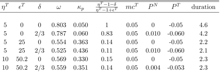
Table 1 reports parameterisations that all imply a slope of the Phillips curve of 0.05. For a given elasticity of in‡ation to real marginal cost, the presence of a variable demand elasticity allows for more reasonable contract duration as emphasised in Woodford (2005): here it comes down from 4.6 to 2.2 quarters. Without a distribution sector, all the parameterisations are observationally equivalent in terms of in‡ation dynamics: the coe¢ cients of the marginal cost and of the traded good price are the same whatever the choice of demand elasticity and curvature. In the presence of a distribution sector, both the weight on the price of non-traded goods and the weight on the price of traded goods vary with the steady-state demand elasticity. For example, assuming a steady-state mark-up of 25 p.c. and a curvature para-meter, T = 25, where a 1 p.c. increase in relative price leads to a 5.5 p.c. decrease in relative demand, or assuming a lower steady-state mark-up of 11 p.c., i.e. a doubling of the demand elasticity, and choosing a curvature parameter such that a 1 p.c. increase in relative price also causes a doubling of the loss of market share - from 5.5 to 11 p.c. - leads to di¤erent coe¢ cients for the aggregate price of non-traded and traded goods. This increase in de-mand elasticity in turn leads to a smaller reaction of in‡ation to both prices. However, for a given demand elasticity, these coe¢ cients are the same for all the choices of curvature which makes identi…cation of the individual para-meters impossible. In this case, T 1 is independent of the curvature parameter and the elasticity of in‡ation to marginal cost, p
T 1
T 1+T has
been constrained to be 0.05 for all speci…cations. Thus, by construction, the ratio p
T 1+T which in combination with and T determines the sensitivity
of in‡ation in the traded goods sector to the aggregate price of non-traded and traded goods is the same for all degrees of curvature once and T are
Table 1:
Combinations of parameters that yield the same Phillips curve slope
T T !
p
T 1
T 1+T mc
T PN PT duration
5 0 0 0.803 0.050 1 0.05 0 -0.05 4.6
5 0 2/3 0.787 0.060 0.83 0.05 0.010 -0.060 4.2 5 25 0 0.554 0.363 0.14 0.05 0 -0.05 2.2 5 25 2/3 0.525 0.436 0.11 0.05 0.010 -0.060 2.1 10 50.2 0 0.569 0.330 0.15 0.05 0 -0.05 2.3 10 50.2 2/3 0.559 0.351 0.14 0.05 0.004 -0.053 2.3
4
Parameterisation and functioning
of the model
4.1
Parameterisation
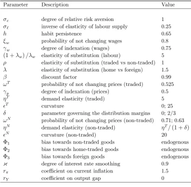
This section is didactical and does not claim to be empirically realistic. An empirical validation of the model is left for further work. To make the expla-nation of the functioning of the model easier, I use a hypothetical symmetric two-country economy: Home and Foreign countries have the same size and parameter values. These parameters are summarised in table 2. A time period in the model is taken to be a quarter.
A low degree of relative risk aversion ( c = 1) and a high elasticity of
labour supply ( l = 0:25) are chosen. The habit persistence parameter is
…xed at 0.65. The subjective discount factor equals 0.99. The parameter capturing the mark-up in wage setting is set at w = 0:25.
The 0sare endogenously chosen to ensure that, at steady-state, whatever the size of the distribution sector, the shares of non-traded, of home-traded and of imports in GDP remain respectively at 0.5, 0.25 and 0.25. There is thus no home bias in traded goods: 2
2+ 3 = 1=2:
The elasticity of substitution between domestic and imported goods is set at 1.5 as in Chari et al.16 (2002) and the elasticity of substitution between traded and non-traded goods is set at 1 as in many theoretical papers. This is above the value of 0.74 suggested by Mendoza (1995) but, here, these substitution possibilities only concern the traded versus non-traded as …nal goods while the overall substitution is quite lower given the fact that non-traded goods are complementary to non-traded ones in the form of distribution
services.
I measure the distribution margin as a fraction 1+ of the retail price. Thus a 40 p.c. margin implies a value of 2/3 for the parameter as the remaining 60 p.c. of the retail price represents the wholesale price. In this model, the distribution sector is assumed to be competitive, so economic pro…ts are zero and the distribution margin re‡ects the costs associated with providing distribution services. If the distribution sector is monopolistically competitive, the distribution margin also includes a mark-up component, as in Corsetti et al. (2007).
The variable demand elasticity is parameterised by ensuring that net mark-ups are equal to 0.25 across sectors at z(i) = 1. In the traded sector, the curvature parameter is chosen so that a 2 p.c. increase in price reduces demand by 11.9 p.c. as compared to 10 p.c. in the CES case. The proba-bility of not changing prices is set at 0.525, implying an average duration of 2.1 quarters in the traded sector. In the non-traded sector, where nominal stickiness is larger according to Alvarez et al. (2005); the parameter is cal-culated to ensure that a weight on marginal cost in the in‡ation equation is close to 0.02 in both speci…cations with and without the distribution sector, a value commonly obtained in estimating the New Keynesian Phillips Curve. In combination with a curvature parameter set at 20, it equals 0.71 with the distribution sector and 0.63 without, corresponding to average durations of respectively 3.4 and 2.7 quarters. The indexation parameters are set at 0.5 for prices and 0.75 for wages.
Table 2: Parameter Values
Parameter Description Value
c degree of relative risk aversion 1
` inverse of elasticity of labour supply 0.25
h habit persistence 0.65
w probability of not changing wages 0.8
w degree of indexation (wages) 0.75
(1 + w)= w elasticity of substitution (labour) 5
elasticity of substitution (traded vs non-traded) 1 elasticity of substitution (home vs foreign) 1.5
discount factor 0.99
!T probability of not changing prices (traded) 0.525
p degree of indexation (prices) 0.5
T demand elasticity (traded) 5
T curvature 0; 25
parameter governing the distribution margins 0; 2/3 !N probability of not changing prices (non-traded) 0.71; 0.63
N demand elasticity (non-traded) T=(1 + )
N curvature (non-traded) 20
1 bias towards non-traded goods endogenous
2 bias towards home-traded goods endogenous
3 bias towards foreign goods endogenous
{ degree of interest rate smoothing 0.9
r coe¢ cient on current in‡ation 1.5
rY coe¢ cient on output gap 0
4.2
Functioning of the model: Impulse responses to
shocks
4.2.1 Uncovered Interest Rate Parity shock
This subsection compares impulse responses to a Uncovered Interest Rate Parity shock in four alternative speci…cations. First, I look at nominal rigidi-ties only. Then, real rigidirigidi-ties are introduced separately. The impact of dis-tribution costs is considered …rst. I consider the case with distributive trade, >0, but the demand function is still of the CES type by setting T to zero
in the demand for traded goods. Then, I look at a variant of the model with a variable demand elasticity, T >0, but without distribution margins, = 0.
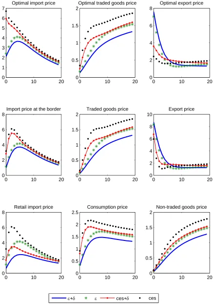
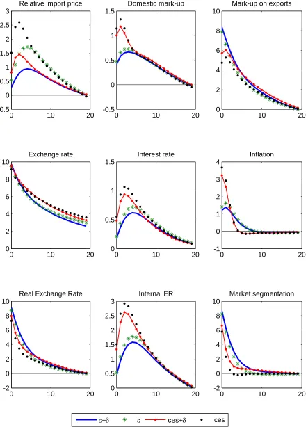
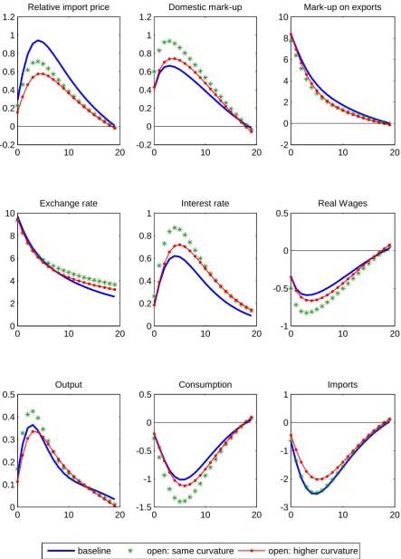
bas-are directly bought by consumers from non-traded producers. Finally, the model incorporates the real rigidities together. The full model is represented by a bold continuous line, the model without distribution services by stars ’*’, the CES variant by the combination of a thin line and points ’’and the model with only nominal stickiness by points ’’.
The size of the shock is scaled so that it triggers a 10 p.c. depreciation of the Home country exchange rate. It is assumed to be fairly persistent ( = 0:9) with its e¤ect on the real exchange rate dying out only slowly over time. It a¤ects both economies in a perfectly symmetric way. Because the model is symmetric, I concentrate on the results for the Home economy.
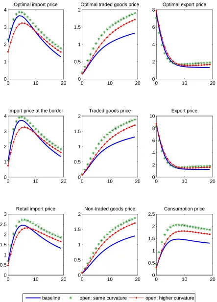
Firms’ reactions: The …rst row of Figure 1 displays the optimal prices charged by Foreign price-adjusting …rms on the Home market, called optimal import price (at the border), as well as the optimal wholesale prices charged by Home price-adjusting …rms on Home and Foreign markets. The second row gives the respective price index accounting for …rms which cannot adjust their price. All prices are expressed in the Home currency.
Of course, …rms would prefer to change their price in response to the exchange rate or cost changes. However, in the Calvo framework they can only do so when they receive the price "signal". There is thus some gradual adjustment in all cases. In the presence of only nominal rigidities, both the domestic optimal traded good price and the optimal price of Home goods sold abroad increase slightly. On impact, the price that exporting …rms are charging increases by some 2.4 p.c. This price increase then improves the Home-traded goods …rms’margins. Given that the exchange rate appreciates by 10 p.c., this movement means that, once expressed in foreign currency, the price of domestic goods sold abroad falls by some 7.6 p.c., implying a high degree of pass-through.
When real rigidities are introduced, the optimal price of home-traded goods does not increase as much. On the contrary, the optimal export price increases even further: 3.6 p.c. when distribution is added, 7 when the demand elasticity is variable and 7.6 when both real factors are taken into account. The fact that domestic …rms set two di¤erent prices at Home and abroad is a clear illustration of how market segmentation breaks the link between Home and Foreign demand and enables …rms to price to market.
trans-lates into optimal price very gradually as re-optimised individual prices feed into the aggregate price and reduce the impact of price adjustments on mar-ket share. In contrast, when the elasticity of demand is constant …rms which can re-optimise are less reluctant to raise (reduce) their price more on impact since they do not consider the impact of charging a higher (lower) price than their competitors.
When the distribution margin is set at 40 p.c. instead of zero, there is a smaller increase in both the optimal Home price of traded goods and in the optimal Home currency price of imports. As noted, an increase in lowers the "perceived" demand elasticity faced by traded goods producers and reduces the exchange rate pass-through to the wholesale price. Thus, exporters reduce their price in foreign currency by less than they would when is zero. As a result, once expressed in Home currency, export price further increases.
As expected, raising the demand elasticity, i.e. reducing , increases the exchange rate pass-through on optimal prices: Home producers’export price falls more in Foreign currency and Foreign producers’ export price on the Home market increases more in Home currency. In addition, the di¤erence is even greater under the CES speci…cation. As explained above, when T >0
producers of tradables reduce their response to an increase in the price set in the non-traded sector because they have less margin for increasing their price given that the variable elasticity rises as their relative prices rise. The e¤ect of distributive trade is thus relatively smaller when the elasticity of demand is increasing with the relative price.
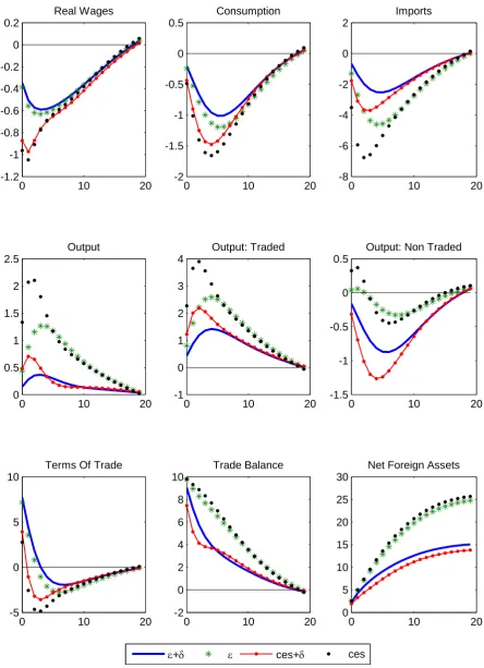
This being said, the most striking di¤erence introduced by distribution trade is its impact on the retail price of import and on the expenditure-switching e¤ects it generates.
eign currency induce a shift in demand towards domestic traded goods so that net exports improve substantially17. On the other hand, the current or expected deterioration in the terms of trade generates a negative wealth e¤ect. Moreover with the simple monetary policy rule as in (35), the in-terest rate increases and consumption decreases. All in all, following the depreciation, Home output increases.
Although import prices "at the border" change the most with the CES ag-gregator, variations in net exports do not follow the same ranking. Expenditure-switching e¤ects are in fact conditioned by the "retail" price of imports as in (11) where import demand depends on PT D
F . Given that the "retail" price
increases less in the presence of distributive trade, import volumes decrease less and their mirror image, export volumes, increases to a lesser extent. In addition, when distributive trade is added to the model, output in the non-traded sector falls even more sharply following the depreciation: there is a reduction in demand for non-traded goods used as retail services. There is also a limited increase in demand as a result of a reduction in non-traded output combined with a much lower net export improvement.
In the variants in which producers set prices while striving to maintain competitiveness against other producers, all price e¤ects are smaller. In particular, the consumer price increases less and the response of monetary policy is less aggressive which results in a lower real interest rate. This induces a smaller reduction in consumption.
However, the striking di¤erence in the output responses stems from the non-traded sector. In both scenarios with a distribution margin, there is a marked reduction of output in the non-traded sector accompanying the fall in imports. This reduction in distributive trade combined with a compres-sion of domestic consumption keeps output almost at steady state despite the increase in exports. Without distributive trade, not only do net export improves more but also the decrease in the production of non-traded goods is very limited, which tends to boost domestic output.
Let us de…ne the terms of trade as the ratio of the Home-currency price received on home goods exported abroad over the Home-currency price paid for goods imported from abroad. Under traditional Keynesian sticky-price models, the terms of trade decrease following domestic currency depreciation as the home-currency price paid for goods imported increases while the price received for exports does not change. Obstfeld and Rogo¤ (2000) provide empirical evidence of a negative comovement between the nominal exchange
17The chosen value for the elasticity of substitution (1.5) may be responsible for the
rate and the terms of trade ( a weaker currency is associated with a worsen-ing of the terms of trade) and use it against the LCP hypothesis. Conversely, Bergin (2006) carries out a maximum likelihood estimate of a two-country model on US and G7 data and …nds that a large proportion of …rms be-haves according to the assumption of Local Currency Pricing. In the current Pricing-To-Market environment, currency depreciation causes a temporary improvement of the terms of trade in all three cases where real rigidities come on top of the nominal price stickiness. Therefore, although the model generates a positive e¤ect on the trade balance on impact, terms of trade movements contradict Obstfeld and Rogo¤’s argument.18 However, after 3 quarters at most (when demand elasticity is variable), the model starts to show some deterioration in the terms of trade as the price paid for imported goods is above the price received for exported goods.
What drives RER movements? The real exchange rate ‡uctuates if Home and Foreign price levels are not perfectly correlated and an imperfect ERPT breaks this perfect correlation. Given that the movements in CPIs are larger under the CES speci…cation, the real exchange rate depreciates some-what less on impact than in the cases with a variable elasticity of demand.
Although the real exchange rate is by and large similar across the four models, the underlying factors explaining its movements di¤er considerably. In log deviations, the real exchange rate is: rsb = bs+Pb Pb. Working in …rst di¤erences and substituting Home in‡ation, , by (34) and by the similar expression for the foreign economy, after some further manipulations, one can decompose changes in the real exchange rate as follows19:
b
rs = 1+1+ ( 2+ 3) 1+ ( 2+ 3)
(0:5)
bN bT 1+ 1+ ( 2+ 3)
1 + ( 2+ 3) (0:5)
bN bT
+
0 B @ 2
2+ 3
(0:5)
3
2+ 3
(0:5)
1 C
A bTF b T H
+ 2
2+ 3
(0:5)
bT F b
T
F + bs +
3
2+ 3
(0:5)
bT H b
T
H + bs
(38)
18The addition of oil or commodities that are priced in a foreign currency could easily
make the model conform more closely with Obstfeld and Rogo¤ views.
Benigno and Thoenissen (2003) label these three sources of variation as:
rs = Internal Exchange Rate
+ Home bias
+ M arket Segmentation
Note that, due to the presence of distribution services, the ratio of Home and Foreign import prices in Benigno and Thoenissen (2003) has been fur-ther decomposed into the contribution of the import price "at the border" and of the distribution services needed to bring imports to the …nal de-mand. These distribution services constitute an additional (indirect) chan-nel through which changes in non-tradable prices a¤ect the (internal) real exchange rate.
The Internal Exchange Rate channel allows the real exchange rate to devi-ate from PPP through the presence of non-traded goods in the consumption basket both as …nal consumption goods and as distribution services. The former is represented by the terms involving 1 and 1 in the …rst row of
(38), while 1+ and 1+ account for the latter. Thus, the higher the impor-tance of the non-traded goods, the larger the real exchange rate sensitivity to changes in the relative price of non-tradables. As can be seen from the lower panel of Figure 1-c, this channel is responsible for twice as large a real exchange rate depreciation in the model with a constant demand elasticity than in the other two variants. In the CES cases, since traded goods …rms do not aim to preserve their market share, they set prices more aggressively so that in‡ation in the Home-traded sector increases more and the relative price of non-traded goods thus decreases more.
The market segmentation channel highlights di¤erences in prices in the same currency of traded goods across countries. In terms of level, market segmentation allows …rms to price-to-market. If …rms face di¤erent elastici-ties of demand in di¤erent markets as in the presence of distributive trade, this causes absolute PPP to fall. In the transitional dynamics depicted in the impulse responses, this channel a¤ects the real exchange rate because there is incomplete pass-through from the exchange rate to prices so that the law of one price does not hold. As seen by comparing Figure 1-a and 1-c, the lower the exchange pass-through, the greater the contribution of the market segmentation channel. On the contrary, if the pass-through is perfect (which is the case, for instance, in the Producer Currency Pricing model), this channel would not contribute to the variability of the real exchange rate. The home bias channel allows the real exchange rate to deviate from PPP through changes in the price of imported goods relative to those of the domes-tic tradable goods. The higher the degree of home bias, 2
2+ 3
3