The MRE inverse problem for the elastic shear modulus

MODULUS∗

PENNY J DAVIES†, ERIC BARNHILL‡,AND INGOLF SACK‡

Abstract. Magnetic resonance elastography (MRE) is a powerful technique for noninvasive determination of the biomechanical properties of tissue, with important applications in disease di-agnosis. A typical experimental scenario is to induce waves in the tissue by time-harmonic external mechanical oscillation and then measure the tissue’s displacement at fixed spatial positions 8 times during a complete time-period, extracting the dominant frequency signal from the discrete Fourier transform in time. Accurate reconstruction of the tissue’s elastic moduli from MRE data is a chal-lenging inverse problem, and we derive and analyze two new methods which address different aspects. The first of these concerns the time signal: using only the dominant frequency component loses in-formation for noisy data and typically gives a complex value for the (real) shear modulus, which is then hard to interpret. Our new reconstruction method is based on the Fourier time-interpolant of the displacement: it uses all the measured information and automatically gives a real value of shear modulus up to rounding error. This derivation is for homogeneous materials, and our second new method (stacked frequency wave inversion, SFWI) concerns the inhomogeneous shear modulus in the time-harmonic case. The underlying problem is ill-conditioned because the coefficient of the shear modulus in the governing equations can be zero or small, and the SFWI approach overcomes this by combining approximations at different frequencies into a single overdetermined matrix–vector equation. Careful numerical tests confirm that both these new algorithms perform well.

Key words. Magnetic resonance elastography (MRE), elasticity, biomechanics, inverse problem

AMS subject classifications. 74L15, 74530, 35R30

1. Introduction. Magnetic resonance elastography (MRE) is a powerful tech-nique for noninvasive determination of the biomechanical properties of tissue, with important applications in disease diagnosis (as described e.g. by [17,8,7,5]). Waves are induced in the tissue (typically by external mechanical excitation) and the result-ing tissue displacement is measured at fixed sitesinside it using phase-contrast MRI. This is unlike surface-based mechanical tests which can induce and measure mechan-ical strain only at surfaces, and thus MRE provides a far richer data source. Despite this, accurate reconstruction of the tissue’s elastic moduli is still a challenging inverse problem, with many different methods proposed (see e.g. [15, 18, 17,19,8]).

Here we propose and analyze a new method which is based on and closely related to the recently introduced heterogeneous multifrequency direct inversion (HMDI) method [5]. The advantages of the new method, which we term stacked frequency wave inversion (SFWI), are that it needs only first derivatives of the wave displace-ment (HMDI uses second derivatives) and the shear modulus is obtained directly from a least squares solve. The “frequency domain” (time-harmonic) version of SFWI is de-scribed and analyzed in Secs.4–5, but in practice MRE data are sampled at (typically) 8 times per time-period and the dominant frequency signal induced by the mechanical oscillations is extracted from the discrete Fourier transform (DFT) in time. The two main disadvantages of this approach are (i) that it results in a loss of information for noisy data, and (ii) using only one Fourier component typically gives a complex value for the (real) shear modulus, which is then hard to interpret. In Sec. 2 we

∗_{Revised version: April 24, 2019.}

Funding:This work was supported by the German Research Foundation (GRK2260, BIOQIC).

†_{Department of Mathematics and Statistics, University of Strathclyde, 26 Richmond St, Glasgow,}

G1 1XH, UK (penny.davies@strath.ac.uk)

‡_{Department of Radiology, Charit´e-Universit¨atsmedizin, Berlin, Germany (} ericbarn-hill@gmail.com,ingolf.sack@charite.de)

describe a new reconstruction method which is based on the Fourier time-interpolant of the displacement. It uses all the measured information and automatically gives a real value of shear modulus up to rounding error. Our derivation is for the homo-geneous (constant modulus) problem and we thoroughly test it on “synthetic” and experimental data. Future work will extend the method to a SFWI algorithm for the inhomogeneous reconstruction problem, but we note that several existing methods use a “locally homogeneous” assumption (as described in e.g. [5, Sec. 1]) to which this new Fourier interpolant approach could be applied directly.

Unsurprisingly our results show that the shear modulus inverse problem is sen-sitive to noise in both the homogeneous and inhomogeneous case. In some sense signal denoising is the “elephant in the room” of MRE reconstruction, with published methods often being applied to highly polished data, with little information on the procedures which have been applied (note that full details of processing are given in [5]). It is clear that denoising is essential to obtain reliable results from experimental data, although it is hard to test its impact on synthetic data to which noise has been artificially added. For example, simply adding in a “random” error and then filtering it out again before running a reconstruction algorithm is unlikely to yield any insight as to the algorithm’s performance on experimental data, with or without denoising. For this reason our synthetic simulations just consider the effect of added noise on the end result, rather than the effect of added noise with denoising.

It is well-known that waves are attenuated as they pass through tissue, and the ab-sorption of energy is typically frequency-dependent (see e.g. [12]). This phenomenon can be modeled (at least for some frequency ranges) by adding in non-local terms which involve fractional derivatives in time or space. We do not consider this aspect here, focusing attention on methods to calculate parameters for the elastic wave equa-tion. Suppose that measurements are taken in ΩL ⊂Rd for d= 2 or 3, where Lis

a typical length scale – in applications ΩL is a rectangle or box with sides of length

O(L). The displacement u(x, t) of an elastic material at timet of a point originally atx∈ΩL satisfies the momentum balance equations

(1.1) ρu¨ = divT ,

whereρis the material’s density, an overdot denotes the total derivative with respect to time, T is the stress tensor corresponding to the displacement u, and we assume that body forces such as gravity are small enough to be ignored. The divergence of a tensor is the vector with αth component (divT)_α=∂Tαβ/∂xβ =Tαβ,β (the comma denotes a space derivative), and we use the summation convention in which a repeated index (hereβ) means that the expression is summed from 1 :d.

The displacementuis assumed to be small enough for a linear model to be valid, and we also assume that the material is isotropic (i.e. there is not a preferred direction, unlike muscle fibers). In this case the stress isTαβ=λ uγ,γδαβ+µ(uα,β+uβ,α) and (1.1) is the elastic wave equation (EWE)

(1.2) ρ¨uα= (µ(uα,β+uβ,α)),β+ (λ uβ,β),α forα= 1 :d,

whereλ(x) andµ(x) are Lam´e material parameters (µis the shear modulus). In the homogeneous case (i.e. bothλand µare constant) the EWE admits lon-gitudinal and transverse plane wave solutions: a lonlon-gitudinal (pressure) wave with speedcp =

p

(λ+ 2µ)/ρand transverse (shear) waves with speed cs= p

µ/ρ. Both

used in MRE (up to a few hundred Hz), this gives a wavelength of the order of several metres, which is undetectable and so longitudinal waves are removed from (1.2) in MRE applications. The Helmholtz decomposition [10] gives u∈Rd ford= 2 : 3 as

the sum of a gradient and a curl, and filtering out the gradient part ofuin (1.2) gives the shear wave equation (SWE)

(1.3) ρu¨α= (µ(uα,β+uβ,α)),β forα= 1 :d,

where now divu = 0. We follow [15] in using this simplified version of the MRE problem, but note that it is a less accurate model than the approach of [17], where

p≡λdivu is taken to be an unknown pressure term and measured values ofu are used to determine both µ and pfrom (1.2). An alternative approach using the full equation (1.2) for piecewise homogeneous materials is developed in [2].

It is known thatµvaries widely in body tissues and reported values of the shear wave speed [16, Table 4] place it roughly in the range 1–20 m/s, giving a measurable wavelength at typical MRE oscillation frequencies. Our MRE reconstruction problem is then to determine the (inhomogeneous) shear modulus µ from (1.3) using space– time measurements ofu. As noted above, a typical experimental scenario is to vibrate the tissue at a known frequencyf (for example by placing the subject on a vibrating surface), measuringuat fixed spatial positions in ΩL at 8 time-steps per period, and the dominant frequency data is typically extracted by taking the DFT in time of the measured displacement and then fitted to the frequency domain PDE obtained by replacing ¨uby (2πf)2_{uin (1.3). We first nondimensionalize the SWE (1.3), setting:}

x=Lx˜, t= ˜t/(2π f), µ(x) =µ0µ˜(˜x), and u(x, t) = ˜u(˜x,˜t),

whereµ0 is a constant of the same order of magnitude asµ, so that ˜µ(˜x) is anO(1) quantity. Dropping the tildes from all terms then gives the nondimensionalized SWE

(1.4) ¨uα=c2 (µ(uα,β+uβ,α)),β forα= 1 :d, for (x, t)∈Ω1×(0,2π) ,

where

(1.5) c2= µ0

ρ L2_{(2π f)}2 .

We derive and analyze the new SFWI method for the inhomogeneous reconstruc-tion problem ofµfromuin Secs4–5 for the frequency domain case

(1.6) −uα=c2 (µ(uα,β+uβ,α)),β forα= 1 :d, forx∈Ω1.

Before this we consider the homogeneous version of the time-dependent problem (1.4).

2. Homogeneous reconstruction problem. In the homogeneous case we set the scaling parameterµ0 equal to the (constant) shear modulus, and the problem is then to determine the wave speedcin

(2.1) u¨ =c2 ∇2u+ grad (divu)

The displacement uin MRE reconstructions is typically sampled at 8 times per time-period (which is far too coarse a timestep to use in a central difference approxi-mation of ¨uin (2.1)) and it is standard practice to take its DFT and use the Fourier component which corresponds to the underlying oscillation frequency. This throws away potentially useful information and typically gives a complex value of the real quantityµ0, and instead we derive a new MRE inversion procedure which uses Fourier interpolation in time. The new method is extensively tested on “synthetic” problems in 1D and 2D space and also used for 3D MRE data in Sec3.

2.1. Homogeneous problem in 1D. The 1D model problem is to findcsq≈c2 to best fit measured values of the 2π-periodic in time functionu(x, t) which satisfies the underlying equation

(2.2) utt=c2uxx, x∈(0,1).

Our strategy is to replaceuin (2.2) by its (time) Fourier interpolant, and we first de-scribe this construction, which follows the approach of Trefethen [20], before detailing the full approximation method forcsq.

Fourier interpolant in time. Suppose thatv∈C[0,2π] is a 2π-periodic func-tion measured attm=mhform= 0 :M−1 whereh= 2π/M, and setvm=v(tm). The discrete Fourier transform (DFT) ofvis_bv` : `=−M/2 + 1 :M/2 , where

b

v`= M−1

X

m=0

e−i`tm <sub>v</sub>m<sub>, `=−M/2 + 1 :M/2</sub>

and the inverse DFT is

vm= 1

M

M/2 X

`=−M/2 0 <sub>e</sub>i`tm

b

v`, m= 0 :M−1,

where_bv−M/2=_bvM/2_{and the prime on the sum indicates that terms with`=±M/2} are multiplied by 1₂ . The Fourier interpolant of visV(t) defined by

V(t) = 1

M

M/2 X

`=−M/2 0<sub>e</sub>i`t

b

v`.

It is an analytic function oft andV(tm) =v(tm) for eachm by construction. Differ-entiating twice in time att=tmgives

(2.3) V¨(tm) = 1

M

M/2 X

`=−M/2+1

−`2<sub>e</sub>i`tm

b

v`, m= 0 :M−1.

As noted in [20, Ch. 3], if the way the DFT is implemented assumes a different ordering of the wavenumbers then the vector of multipliers of the components −`2 _{will also} need to be reordered. For example, if using_Matlab’sfftfunction to overwrite the

Least squares approximation ofc2_{. The measured displacement is the average} value over a voxel, and so in 1D space it corresponds to the average over an interval of length ∆x = 1/J, i.e. the measurement um

j ≈ u(xj−1/2, tm), where xr = r∆x. Approximatinguin (2.2) by its Fourier interpolantU at each space–time measurement point (xj−1/2, tm) andUxx by a second central difference gives

1 M M/2 X `=−M/2+1

`2<sub>b</sub>u`j+c2

δ11 ∆x2 bu

` j

ei`tm _{≈0 for eachmandj ,}

whereδ11gj=gj+1−2gj+gj−1. Hencecsq≈c2is the best least squares solution of

`2u<sub>b</sub>`_j+csq

δ11 ∆x2 bu

`

j = 0 over`andj .

To calculate csq we multiply this expression by the complex conjugate bu `

j and sum over all indicesj for which the term δ11bu

`

j makes sense (j = 2 : J−1) to give the least squares problem:

(2.4) findcsq≈c2 to minimizekacsq−bk,

wherea,b∈RM have components

(2.5) a`=− J−1 X

j=2 _δ

11 ∆x2 ub

` j

b

u`<sub>j</sub>, b`=`2 J−1 X

j=2 _bu`_j

2

for`=−M/2 + 1 :M/2.

In practice (using floating point arithmetic) it can be more accurate to use “summation by parts” to replace the first sum by the product of first differences:

(2.6) − J−1 X j=2 _δ 11 ∆x2 ub

` j

b

u`_j = J−2 X

j=2 Du_b`_j

2

+Du_b`<sub>1</sub> ub ` 2 ∆x−Dub

` J−1 b

u`_J−1

∆x ,

where D_bu` j = bu

` j+1−ub

` j

/∆x. We always do this, but because the formula for a term like a` is far simpler written as a second difference (especially in higher space dimensions), we will not in general give the equivalent first difference form explicitly. Note that the approximation c∗_sq of c2 _{given by the Helmholtz approach (1.6)} is obtained from a single Fourier component of (2.4) rather than the least squares solution over allM Fourier components, i.e. it is

(2.7) c∗_sq=b`∗/a<sub>`</sub>∗

for the dominant frequency`∗.

2.2. Homogeneous problem in 2D. The 2D homogeneous model problem uses measured values of u ∈ _R2 _{in (2.1) to determine c}

terms. The approximation used for mixed partial derivatives is ∂12g ≈δ12g/∆x2, where

δ12gp,q= [gp+1,q+1−gp−1,q+1−(gp+1,q−1−gp−1,q−1)]/4.

Using these approximations in (2.1) leads to an expression like (2.6) for each spa-tial component of u and taking the scalar product with the complex conjugate of

b

u` 1[j,k],ub

` 2[j,k]

and summing overj = 2 :J1−1 andk= 2 :J2−1 again gives the least squares problem (2.4) forcsq≈c2, where now for each`we havea`=a

[1] ` +a

[2] ` for

a[1]_` = −1 ∆x2

J1−1

X

j=2 J2−1

X

k=2

2δ11_bu`1[j,k]+δ22<sub>b</sub>u`1[j,k]+δ12_bu`2[j,k]

b

u`_1[j,k],

a[2]_` = −1 ∆x2

J1−1

X

j=2 J2−1

X

k=2

δ11_bu`2[j,k]+ 2δ22u<sub>b</sub>`2[j,k]+δ12_bu`1[j,k]

b

u`_2[j,k],

and b`= J1−1

X

j=2 J2−1

X k=2 bu ` 1[j,k] 2 + bu ` 2[j,k] 2 .

3. Numerical results for the homogeneous problem. We now present nu-merical test results for the time-dependent homogeneous problem. We use ‘synthetic’ data (with and without added noise) in one and two space dimensions and unsmoothed MRE measurements in 3D. The simplicity of the 1D case allows the algorithm to be extensively tested, with and without added noise, revealing insights that are useful for higher space dimensions. It is well-known that noisy MRE data can cause the computed solution to be severely underestimated (see e.g. [4]), and we investigate how this depends on the underlying wave speed.

3.1. Results for synthetic 1D data. The functionu(x, t) = cos(t+x/c) is an exact 2π-periodic solution of (2.2), and we consider a noisy version of it setting

(3.1) um_j = cos(tm+xj−1/2/c) +εmj , j = 1 :J, m= 0 :M−1,

where eachεm_j ∈[−ε, ε] for 0≤ε ≤0.1 is a pseudo-random error term to simulate experimental error. We use these values ofum_j to calculate the vectorsaandbin (2.5) and then findcsq≈c2which satisfies (2.4). The absolute error inc2isEA=csq−c2, and the relative error isER=EA/c2.

We first examine the behavior of the calculated value csq with no added noise (i.e. (3.1) with ε = 0). In this case u is analytic and M = 8 is enough to capture its complete time behavior, and the calculated value csq does not change as M is increased. Figure3.1illustrates the behavior ofcsqwithJ= 1/∆x– the leading term of the absolute error is ∆x2_{/12 and further investigation indicatesE}

A ≈∆x2/12 +

101 102 103 10-8

10-6 10-4

c2 = 0.0001

101 102 103

10-8 10-6 10-4

c2 = 0.1

101 102 103

10-15 10-10 10-5

c2 = 0.0001 c2 = 0.01 c2 = 1

Fig. 3.1. Error plots forcsqreconstructed from the data (3.1) withε= 0andM= 8.

10-5 10-4 10-3 10-2 10-1

4.11 4.12 4.13 4.14

4.15 10

-5 _c2 _{= 0.0001}

J = 50

10-5 10-4 10-3 10-2 10-1

noise ( ) 0.5

1 1.5 2

2.5 10

-6

J = 200

Fig. 3.2. Absolute errorEA withc2= 10−4 andM= 8for 100 simulations at each synthetic

noise levelε.

10-5 10-4 10-3 10-2 10-1

-2 -1 0 1 10

-3 _c2 _{= 0.01}

J = 50

10-5 ₁₀-4 ₁₀-3 ₁₀-2 ₁₀-1

noise ( ) -10

-5 0 5 10

-3

J = 200

Fig. 3.3. Absolute errorEA withc2= 10−2 andM= 8for 100 simulations at each synthetic

Whenε >0 the underlying functionuis no longer analytic, but increasingM still makes very little difference to the reconstruction accuracy and we fix M = 8. The dependence of the absolute errorEAonJ andεis illustrated in Figs3.2–3.3, and each plot showsEAat 100 simulations for a given noise levelε, calculated directly from the data (3.1) with no filtering or smoothing. When εis small compared with ∆x, then the results are similar to theε= 0 case above withEA=O(∆x2), but|EA|increases rapidly with increasing noise level ε, and typically then behaves worse as the mesh is refined (because the approximation error in the first derivative termsD_bu`_j in (2.5) is proportional to ε/∆x). The onset of this rapid growth of |EA| withεdepends on

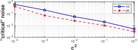
c2, with small values ofc2 (corresponding to a high spatial wavelength) giving better results. For example, the error whenc2_{= 10}−4 _{reduces asJ is increased (the bottom} plot of Fig.3.2shows a 1% relative error at 10% noise), whereas whenc2_{= 10}−2 _the error is about ten times larger when J = 200 than it is atJ = 50. In all cases the rapidly growing error corresponds to an underestimate of the true solution. It is well-known in the MRE community that noisy data causes the shear modulus to be underestimated (see e.g. [4]), and our simulations allow this to be quantified. Fixing

J = 100 andM = 8, we calculate the average value ofcsq over 100 runs at each of a set of noise levelsε≤1 and wave speedsc2_{= 10}−k _{fork= 0 : 4. The ‘critical’ noise} level εcr at each wave speed is defined to be that at which the relative error in csq first reaches 0.1 (i.e. 10%), and a log–log plot of εcr against c2 (see Fig. 3.7) shows thatεcr≈A1c−1 forA1 independent ofc.

Note that the formulation (2.4) automatically gives a real value of csq (up to rounding error), but this isnottrue forc∗sqgiven by (2.7). Although the scatter plots for the error in the real part ofc∗sq look qualitatively similar to Figs3.2–3.3, the ratio of the imaginary and real parts ofc∗sqin these simulations can vary significantly. For example, Fig.3.4shows this ratio plotted against εwhenc2_{= 0.01 – it ranges from} 10−5 to 103_{. A high ratio makes the calculated value ofc}

sq (and henceµ0) very hard to interpret.

10-5 10-4 10-3 10-2 10-1

noise 10-5

100 105

Ratio

c2 = 0.01, J = 50

Fig. 3.4. Ratio of the imaginary and real parts of the absolute error inc∗sq whenc2= 10−2,

J= 50andM= 8for 100 simulations at each synthetic noise levelε.

3.2. Results for synthetic 2D data. The 1D solution u(x, t) = (cos(t+

x1/(c

√

results, and for simplicity we only present results for square pixels. The measured displacement is then the average value over a square of side ∆xwhere ∆x= 1/J1and we record it at the midpoint, setting

uα[j,k](tm) =rαcos

tm+

ν·xj−1/2,k−1/2

c

+εm_j,k,

wherexr,s= (r∆x, s∆x),R2=J2∆xand eachεmj,k∈[−ε, ε] is an added noise term to simulate experimental error.

We first examine the dependence of the absolute errorEA on the space mesh size ∆x and incidence angle θ with no added noise (ε = 0). The results do not appear to depend onc2 _{or the domain’s aspect ratioR}

2/R1, and a sample plot is shown in Fig.3.5. The leading term of the error is again proportional to ∆x2_{, with a constant} of proportionality which is independent ofc2_{but it does depend onθ. This is because} the effective mesh spacing “seen” by the wave depends on its incidence angle – if it is aligned with the mesh (θ = 0 or π/2) then the perpendicular distance between consecutive mesh points is ∆x, but if θ = π/4 then the mesh points are aligned diagonally and their perpendicular distance appears to be ∆x/√2 apart. See e.g. [9] for more information on wave propagation through anisotropic meshes.

0 0.5 1 1.5 2 2.5 3 3.5

-2 0 2

4 10

-5 c

2 = 0.01, J

1 = J2 = J

J = 50 J = 100 J = 200

Fig. 3.5. Absolute errorEAagainst incidence angleθfor a unit square of mesh size∆x= 1/J

whenc2= 10−2 andM= 8.

Fig. 3.6 shows EA at 100 simulations for a given noise level ε, calculated from unsmoothed data at incidence angleθ= 1.3, and usingM = 8 and J1=J2= 100 at two values ofc2_{. These 2D errors are more tightly clustered at each noise level than} the similar 1D plots in Figs.3.2–3.3and for small values ofεthere is a small positive error EA. As in 1D the error drops through zero as ε increases, rapidly becoming large and negative – the bottom plot shows a relative error of ER ≈0.8 (i.e. 80%) when ε= 0.1 (10% noise). The size of the relative error depends on c2, with lower speeds (higher spatial frequencies) giving better results, again as in 1D. E.g. a 10% noise level corresponds to about a 20% relative error whenc2_{= 10}−3_{, and noise levels} of more than 10% are needed to show this behavior whenc2_{= 10}−4_{. The relationship} between the error and noise is illustrated in Fig.3.7; as for the 1D simulations we set

J1=J2= 100,M = 8 and calculate the average value ofcsq over 100 runs at each of a set of noise levelsε≤1 and wave speedsc2_{= 10}−k_{fork= 0 : 4. The ‘critical’ noise} level εcr at each wave speed shown in the Figure is again that at which the relative error in csq first reaches 0.1, and the 2D results areεcr≈A2c−1 where the constant

10-5 10-4 10-3 10-2 10-1 3

4 5 6 10

-6 c2 = 0.0001

10-5 10-4 10-3 10-2 10-1

noise -10

-5 0 5 10

-3 c2 = 0.01

Fig. 3.6. Absolute errorEAfor a unit square of mesh size∆x= 0.01whenθ= 1.3andM= 8

for 100 simulations at each synthetic noise levelεwithc2_{= 10}−4 _{(top) andc}2_{= 10}−2 _(bottom).

10-4 ₁₀-3 ₁₀-2 ₁₀-1 ₁₀0

c2

10-3 10-2 10-1 100

"critical" noise

1D 2D

Fig. 3.7. Critical noise levelεcr at whichER, the relative error incsq, first becomes 10% plotted againstc2 _{for the 1D and 2D simulations. See text for details of the parameters used.}

3.3. Homogeneous problem in 3D. The physical problem for which we have experimental displacement values is that of a cube of size 95×95×95 mm3_of homo-geneous ultrasound gel whose density is close to that for water, which is vibrated at a constant frequencyf. Full details of the experimental procedure are given in [7]. Eight (M = 8) measurements are taken per time period at frequenciesf = 30 : 5 : 60 Hz, giving seven experimental runs in total. The voxel dimensions are 1×1×2 mm, and the full data set covers 128×96×21 voxels (and hence includes “noise” measure-ments in the air as well as measuremeasure-ments from within the cube). Our calculations are based on a data subset ofNv = 75×68×21 voxels giving thex1physical length

L = 75 mm. The measured displacements are nondimensionalized as described in Sec.1, with the three components ofu(·, tm) assumed to be at the center of each voxel for m= 0 : M −1. These samples are all raw data which has not been smoothed, but have been “unwrapped” (from an acquisition in an interval of length 2π) by the Laplacian unwrapper – this suppresses constant offsets or first order gradients (details are given in [7]).

Analysis of data quality. The time behavior of perfect (nondimensionalized) data at a fixed point in space takes the form v(t) =A+ cos(t+B) for constantsA

andB. Measuring it attm,m= 0 :M−1 and taking its DFT as described in Sec.2.1 gives the M-component complex vector v_b where _bv±1 are complex conjugates which contain the signal information, _bv0 _{depends on the translation A and the remaining}

M−3 components_bv` for|`|>1 are all zero. Thus the quantity 1

(M −3)|_bv1_| X

|`|>1

|_bv`|

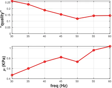
gives an indication of how “good” (i.e. how close to exact periodic) the data values are. This is important because equations (2.4) and (1.6) are both derived under the assumption that the measurements are time-periodic. If this is far from being the case, then it is unclear what the calculated valuescsq orc∗sqactually mean. For each data run we sum up this quality indicator for the three spatial components ofu at all voxels and divide by the total number of terms (3×Nv) to obtain the “quality index”, which is a measure of the signal-to-noise ratio (SNR). It is plotted in Fig.3.8 (top) against (physical) oscillation frequency f: the measurements at 50 Hz appear to be closest to being periodic. Note that there are other ways to evaluate the SNR, for more information see e.g. [4].

30 35 40 45 50 55 60

0 0.05 0.1 0.15 0.2 0.25

"quality"

30 35 40 45 50 55 60

freq (Hz)

0.4 0.6 0.8 1

(KPa)

Fig. 3.8. Top: Quality index against (physical) frequency f. Bottom: Calculated value of (physical) µ0 againstf. Our results are consistent with those (calculated from rheometric data) given in [7, Fig. 4].

Results. We exclude the component with`= 0 in the 3D analogue of (2.5)) in the least squares calculation for experimental data. It is a zero-frequency (constant) mode for whichb0= 0 by definition anda0should also be zero because all its terms involve second differences applied to a constant. Fig.3.8(lower) shows the calculated value of the physical shear modulusµ0 at each experimental run. This is consistent with the values ofµ0(called|G∗|) calculated for this type of gel from rheometric data given in [7, Fig. 4]. For example, the “most periodic” sample at 50 Hz givesµ0= 0.73 KPa, which is within the error bars given in [7] for the rheometric measurements.

reconstruc-tion problem. For simplicity we restrict attenreconstruc-tion to the frequency domain version (1.6), rather than (1.4). The nondimensionalized function µ(x) in (1.6) is an O(1) quantity, and we look at examples in which it is piecewise constant, with inclusions ofµ >1 embedded in a background material for whichµ= 1. We rewrite (1.6) as (4.1) −ω2uα= (µ(uα,β+uβ,α)),β forα= 1 :d, forx∈Ω1,

where the nondimensionalized frequency isω= 2πf Lpρ/µ0. As in Sec.2we analyze the problem in 1D and 2D space, with numerical test results given in Sec.5; 3D results for the related HMDI method are presented in [5].

4.1. SFWI in 1D space. The 1D model problem is to find µ(x) given the nondimensionalized frequencyω and measured values ofu(x) such that

(4.2) −ω2u= (µ u0)0 , x∈(0,1),

where 0 denotes d/dx. This is a first order ODE in µ, which needs one other piece of information, such as a boundary condition, in order to give a unique solution. For example, ifuk(x) are measurements atωk fork= 1 : 2 with bothu0k(0)6= 0, then the general solution of (4.2) can be written as

µ(x)u0k(x) =µ(0)u0k(0)−ω 2 k

Z x

0

uk(s)ds

andµ(0) can be eliminated to obtainµ(x) in terms of theuk. However this is not a practical solution method for noisy data (it gives an ill-conditioned set of equations and poor results). The SFWI approach overcomes this by combining approximations of (4.2) at different frequencies into a single overdetermined matrix–vector equation (see also [3]). Our underlying approximation of (4.2) uses finite volumes based on a staggered grid (uandµare recorded at different grid points), as illustrated in Fig.4.1. The measured displacement is the average over an interval of length ∆x= 1/J, and

uis regarded as being measured at interval midpoints (blue stars). Theµgrid points are interior interval endpoints, i.e.µj ≈µ(xj) forj= 1 :J−1 (red circles).

Fig. 4.1. Staggered grid for 1D approximation of (4.2) on[0,1]: the grid points foru are denoted by blue stars, and those forµby red circles

Equation (4.2) is integrated between each pair of red circles to give

(4.3) [µ(x)u0(x)]xj+1

xj =−ω

2Z xj+1

xj

u(x)dx , j= 1 :J −2.

Then using a central difference approximation for the derivativeu0 and the midpoint rule to approximate the integral term gives the underdetermined linear system

(4.4) Aµ=b

for µ = (µ1, . . . , µJ−1)T, where bj = ω2∆x u(xj+1/2) for j = 1 : J −2 and A ∈

R(J−2)×(J−1)is the bidiagonal matrix with entries

A= 

   

a1 −a2 0 0 . . . 0 0 0 a2 −a3 0 . . . 0 0

..

. ... . .. . .. . .. . .. ... 0 0 0 0 . . . aJ−2 −aJ−1



withaj= u(xj+1/2)−u(xj−1/2)/∆x≈u0(xj) .

We first investigate the structure of the linear system (4.4), summarizing the key results below.

Lemma 4.1. The matrix Ain (4.4) has the following properties.

1. AAT is invertible on its range,R(AAT).

2. Equation (4.4) has a solution if and only ifb∈ R(AAT), and ifb∈ R(AAT)

then the general solution of (4.4) is

(4.5) µ=ATz+ν,

wherez∈RJ−2 is the unique solution ofAATz=bandAν=0.

The proof is straightforward using the following standard result:

Theorem 4.2 (Decomposition; see e.g. [14]). Suppose that B ∈ Rm×n with

m≤n. ThenRn is the direct sum of the range ofBT and the null space ofB, i.e.

(4.6) _Rn=R(BT)⊕ N(B).

Proof of Lemma 4.1.

1. Suppose that AATz = 0 for some z ∈ R(AAT). Then z ∈ R(AAT)∩ N(AAT_{) ={0}by applying Theorem4.2toB=AA}T_{. ThusAA}T _is invert-ible onR(AAT_).

2. It follows from Theorem4.2that_RJ−1=R(AT_{)⊕ N(A), and so ifµ∈}

RJ−1

thenµ=AT_{z+ν for somez∈}

RJ−2 and ν∈ N(A). HenceAµ=AATz,

and if b6∈ R(AAT_{) then (4.4) cannot have a solution. Ifb∈ R(AA}T_{) then} invertibility ofAAT _{guarantees a unique solutionz ofAA}T_z=b.

CharacterizingN(A) is straightforward as described below.

Lemma 4.3. If QJ−1_j=1aj 6= 0 then dim(N(A)) = 1 and N(A) = sp{ν∗} for ν∗ = (1/a1, . . . ,1/aJ−1)T. If QJ−1j=1 aj = 0 then the orthonormal vectors ek with

ak= 0 form a basis for N(A).

Proof. Suppose 0 6= ν ∈ N(A), then it follows from the structure of A that

ajνj−aj+1νj+1= 0 for eachj = 1 :J −2, and soajνj=cfor some constant c. If none of theaj are zero then the only nonzero solution is ν=cν∗. If one or more of theaj are zero thenc= 0 and so ifak 6= 0 then the corresponding componentνk of ν must be zero.

For regions of constantµ(x) the functionu(x) is oscillatory (trigonometric) and hence it is likely that severalaj ≈u0(xj) will be close to zero, withN(A) very sensitive to small perturbations. This means that any attempt to eliminate the null vectorsν from (4.5) using two or more experimental measurements will be doomed to failure. Instead the new SFWI approach combines expressions of the form (4.4) to produce a least squares (overdetermined) system for µ. Suppose that q measurements at a range of frequencies produce the underdetermined systemsA(k)µ=b(k)fork= 1 :q. Setting

(4.7) Ab=



 

A(1) .. .

A(q)





 and bb= 

 

b(1) .. . b(q)



gives the least squares formulation

min µ∈RJ−1

Abµ−bb ,

wherek · kis the 2−norm. Its solutionµ_LS satisfies

b

ATAbµ_LS=AbTbb

(although there are more efficient ways to compute it, see e.g. [11]). We will assume that the matrixAbTAbhas full rank (in practice this is normally the case even forq= 2) and examine the error inµ_LS. The (exact)µ(x) satisfies (4.3) forj = 1 :J−2, and we set µ_ex∈ RJ−1 to be the vector whosejth component is µ(xj), and write (4.3) at frequency ω=ωk as A(k)µex=b

(k)

. Stacking these (exact) matrices and vectors as in the approximate case described above then gives the linear systemAµ_ex=bin

Rq(J−2)×(J−1)whichµexsolves exactly. This means that

b

b−Abµ_ex=bb−b+

A−Ab

µ_ex and so

(4.8) AbTAb(µLS−µex) =AbT

b

b−Abµex

=AbT

b

b−b+AbT

A−Ab

µex.

It is straightforward to verify that the matrixAbTAb −1

b

AT _{is bounded by 1/σwhere}

σis the smallest singular value ofAband this gives the bound

kµ_LS−µ_exk ≤σ−1 kbb−bk+ max|µ(x)| kA−Akb

.

Both norm terms on the right-hand side of this inequality involve the difference be-tweenuin (4.3) and its measurement (noise), and the error involved in approximating the derivative and integral terms in (4.5) to obtain the entries inAbandbbrespectively. See also [1] for MRE inversion error bounds.

4.2. SFWI in 2D space. In 2D space µ(x) solves the 2-component system (4.1), and as in 1D we approximate these equations on a staggered grid at different frequencies, stacking upq >1 underdetermined systems into an overdetermined least squares problem. For simplicity we restrict attention to the case for which Ω1is the unit square; it is split into aJ×J square mesh and again the components ofu are measured at the mesh midpoints (blue stars in Fig. 4.2). Theµ nodes are interior edge midpoints (red circles).

Each component of (4.1) is integrated over each interior square (those bounded by red solid lines in Fig. 4.2), with Ωj,k denoting the ∆x×∆xsquare centered at xj+1/2,k+1/2. Using the midpoint rule to approximate the left-hand integral and the divergence theorem for the right-hand side gives

−ω2_∆x2_u

α(xj+1/2,k+1/2)≈ Z

∂Ωj,k

µ(uα,β+uβ,α)nβ,

where n is the outward unit normal. The midpoint rule is used for the four line integrals on the right-hand side, and any corner components of u are obtained by averaging over the four nearest neighbor midpoint values. For example, when α= 1 the resulting scheme is

Fig. 4.2. Staggered grid for 2D approximation of (4.1) on the unit square: the grid points for

uare denoted by blue stars, and those forµby red circles

where

Tj,k1 = 2

u1_j+1/2,k+1/2−u1_{j−1/2,k+1/2}, Tj,k2 = 2

u1_j+3/2,k+1/2−u1_j+1/2,k+1/2,

T_j,k3 =u1_j+1/2,k+1/2−u1_{j+1/2,k−1/2}+1 4

u2_j+3/2,k+1/2−u2_{j−1/2,k−1/2}+u2_{j+3/2,k−1/2}−u2_{j−1/2,k−1/2}

T_j,k4 =u1_j+1/2,k+3/2−u1

j+1/2,k+1/2+ 1 4

u2_j+3/2,k+3/2−u2_{j−1/2,k+3/2}+u2_j+3/2,k+1/2−u2_{j−1/2,k+1/2},

and for simplicity we writeuβ(xj+1/2,k+1/2) as u β

j+1/2,k+1/2. In total there are 2 (J−2)2_{equations for theN}

J ≡2 (J−1) (J−2) components of the vector ofµvalues, and the underdetermined linear system matrix analogous to

A in (4.4) is again sparse, with 4 nonzero entries per row. As in 1D we stack up q

of these matrix-vector equations, obtained at different frequencies, and calculate its least squares solutionµ_LS∈R2 (J−1) (J−2).

5. Inhomogeneous problem: SFWI results. We now provide numerical test results for the SFWI algorithm using synthetic data in 1D and 2D space. The 1D test results are important in quantifying the algorithm’s behavior in the presence of noise because exact solutions to the inhomogeneous problem are not available in higher space dimensions.

5.1. Numerical results for synthetic 1D data. All tests assume that the (exact)µ(x) is piecewise constant on [0,1] with

(5.1) µ(x) =

1, x∈[0, a)∪(b,1]

µI, x∈(a, b)

and construct the uniqueu∈C1[0,1] which satisfies (4.2) subject to given boundary conditionsu(0) =uL and u(1) =uR. These boundary conditions are fixed in some simulations and varied randomly in others. To simulate experimental error we set the nodaluvalues to beuj =u(xj−1/2) +εj, j= 1 :J , where again eachεj∈(−ε, ε) is a pseudo-random noise term. Tests show that varying the interval parameters (a, b) makes little difference to the results and we fixa= 0.35andb= 0.69.

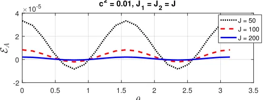
The root mean square (RMS) error in µ(x) is E =kµ√LS−µexk

(large J) at multiple frequencies whenε= 0. Fig.5.1shows that for high resolution the error E is at a minimum when µI = 1 (i.e. the material is homogeneous), and whenµI >1 thenE ∝µ2I. Each entry ofAbin this plot has the same boundary values (uL = −1.156, uR = 0.292), but using boundary values randomly chosen in [−2,2] makes no observable difference.

10-1 100 101 102

10-5

100 = 0, = [10:10:150]

J = 50 J = 200 J = 1000

Fig. 5.1. RMS error inµ(x)plotted againstµI using the frequenciesωk= [10 : 10 : 150]when

J= 50(green dot-dash),J= 200(blue solid) andJ= 1000(red dash).

40 50 60 70 80 90 100

max 0.25

0.3 0.35 0.4 0.45

Fixed BC; = [

min: 10 : max]

min = 20 min = 40 min = 60

Fig. 5.2. RMS errorE plotted against the maximum frequency ωmax for different values of

minimum frequencyωminusing the frequenciesωk= [ωmin: 10 :ωmax]whenJ= 64and noise-level

ε= 0.

0 0.2 0.4 0.6 0.8 1

x

1 2 3 4

(x)

= [40:10:70]

ex

LS

Fig. 5.3. Plot of calculated µLS (red solid line) obtained usingωk ={40,50,60,70} when

J= 64and noise-levelε= 0. The exact valueµexis shown as a a black dashed line.

All further test results use a fixed value of µI = 3 in order to facilitate

com-parisons. In the first of these we look at the effect of varying the maximum and minimum frequencies used to generateAbandbb from (4.7), and results (withJ = 64,

10-5 ₁₀-4 ₁₀-3 ₁₀-2 ₁₀-1 noise

0 0.2 0.4 0.6

0.8 Variable BC; = [40 : 10 : 80]

Fig. 5.4. Plot ofL1-errorE1 inµLSagainst noise-level εobtained usingωk= [40 : 10 : 80]

whenJ= 64. There are 100 simulations at each value ofε.

0 0.2 0.4 0.6 0.8 1

0 2 4 6

(x)

= [40:10:80]; = 0.02

ex

LS

0 0.2 0.4 0.6 0.8 1

x

0 2 4 6

(x)

= [40:10:80]; = 0.04

ex

LS

Fig. 5.5. Plot of 100 simulations of calculatedµLS (red dotted lines) obtained usingωk = [40 : 10 : 80]whenJ= 64and at noise-levelsε= 0.02(top) andε= 0.04(bottom). The exact value µexis shown as a a black solid line in each plot.

(ωmin, ωmax) = (20,60) than (40,60) even though the first of these includes all the frequencies used by the second. This indicates that including a frequency that is “too low” (relative to the mesh spacing) may make the error worse. Using frequencies that are “too high” (relative to the mesh spacing) can be similarly problematic, giving a solution profile that overestimates the value ofµ, and can sometimes be jaggy. The calculated value ofµ_LSfor “intermediate” frequency values is shown in Fig.5.3. This plot was generated using fixed boundary values, but using random boundary values gives similar results. Note that the 1D test problem has a low information content compared with 2D (see below), and far higher frequencies need to be used to obtain reasonable results in 1D.

TheL1-norm is a better characterization thanE of the error that is “seen” in a plot like Fig.5.3and we define

E1= 1

J−1 J−1 X

j=1

(µLS−µex)j .

Fig.5.4 shows the effect of noise, using randomly varied boundary conditions for u

forµ_LSat each ofε= 0.02 andε= 0.04 over these five frequencies with fixed boundary conditions is shown in Fig.5.5.

5.2. Numerical results for synthetic 2D data. The additional difficulty in 2D simulations is in calculatingufor a given inhomogeneousµ(x). This has to be done numerically, and so it is impossible to exactly quantify the noise in a given simulation. All the test results shown below use a piecewise constantµ(x) with background value 1 and valueµI = 3 in a rectangular inclusion with diagonal corners (0.35,0.42) and (0.69,0.65). The functionu(x) which satisfies (4.1) for thisµis calculated using the Matlab PDE toolbox on a regular grid of 2Jf2 triangular elements with Jf = 256 (the maximum size allowed by local computer memory requirements), and synthetic noise of size ε is added, as for 1D. For ease of comparison all simulations use the same boundary conditions for u(x), corresponding to the same incident wave field. The approximation accuracy of the solution u(x) of (4.1) strongly degrades as the nondimensionalized frequency ω increases, but it is notable that calculations using moderate or very low values ofω all give very similar results whenε= 0.

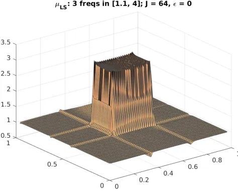
Fig. 5.6. Plot ofµLScalculated usingω= 1.1,2.7,4.0whenJ= 64andε= 0.

Fig.5.6shows the least-squares solutionµ_LS obtained from the three valuesω= 1.1,2.7,4.0 and sample test results for theLp _{errors forp= 1, 2 and∞ whenε= 0} are given in Table5.1, where the errors are defined as follows:

Ep= 

 1

NJ J−2 X

j=1 J−1 X

k=1 µ

(e) j+1/2,k

p

+ µ

(e) k,j+1/2

p



 1/p

forp= 1 : 2

and E∞ = max n

µ

(e) j+1/2,k

,

µ

(e) k,j+1/2

:j = 1 :J−2, k= 1 :J−1 o

ω values used E1 E2 E∞

1.1, 2.7, 4.0 0.024 0.122 1.87 4.0, 7.2, 10.0 0.023 0.121 1.72 10, 17.6, 31.2, 40, 50 0.032 0.102 1.72 17.6, 31.2, 40, 50 0.032 0.102 1.72

31.2, 40, 50 0.033 0.103 1.72

Table 5.1

Calculated errors inµ_LSusing various frequencies whenJ= 64andε= 0.

Fig. 5.7. Plot of errorµ(e) _{calculated usingω= 1.1,2.7,4.0whenJ= 64andε= 0}

Calculations with only low values of ω are very susceptible to added noise, as indicated by Table 5.2. Any values of E1 larger than about 0.2 correspond to an unacceptably bad solution, and the lower frequency calculations (top two rows) are much worse than this even for ε= 10−4. The results in the bottom three rows are acceptable up toε≈0.01.

ω values used ε= 10−4 _{ε= 10}−3 _{ε= 10}−2

(J = 64) E1 E2 E1 E2 E1 E2

1.1, 2.7, 4.0 0.463 0.682 1.074 1.249 1.166 1.292 4.0, 7.2, 10.0 0.059 0.163 0.678 0.946 1.022 1.251 10, 17.6, 31.2, 40, 50 0.032 0.103 0.035 0.105 0.172 0.352 17.6, 31.2, 40, 50 0.032 0.102 0.035 0.105 0.163 0.325 31.2, 40, 50 0.033 0.103 0.036 0.105 0.160 0.322

Table 5.2

Calculated errors inµLSat three different values of added noise.

6. Discussion and conclusions. Reconstructing the elastic shear modulus

MRE measurements are typically taken in small enough space voxels for central differences to give a reasonable approximation of space derivatives, but the relatively coarse timestep size means that an additional assumption of (near) periodicity in time is necessary. The advantages of the Fourier time-interpolant approach (i) are that it uses all the information present in the experimental measurements ofu(x, t) and it is guaranteed to give a real value of the real quantityµ. It is well-known that noisy MRE data causes the shear modulus to be underestimated and the numerical test results of Sec.3quantify this, showing that the solution is insensitive to low values of additional noise, but that when the noise level exceeds a ‘critical’ value, then the error in the calculated shear modulus increases rapidly. This critical noise level is proportional to 1/c where c is the wave speed in (2.1), and the constant of proportionality in 2D is half that for 1D.

The underlying problem (1.6) is ill-conditioned because the coefficients of the shear modulus can be zero or small, and the SFWI method overcomes this by com-bining approximations at different frequencies into a single overdetermined matrix– vector equation. Because the individual matrices are derived at different frequencies they have different “problematic” coefficients (i.e. those equal or close to zero) and the overall stacked matrix has full rank if enough frequencies are used. Note that there is a higher information content in the problem as the space dimension increases and so the method should workbetter (i.e. for lower nondimensionalized frequencies) in 3D space than in 2D space (our numerical tests confirm that it works better in 2D space than 1D). This is in contrast to the forward problem of trying to compute the solutionu of (1.4) or (1.6) from µ. Our method is designed for MRE inverse prob-lems in whichµis not known anywhere in the material, including at the boundaries. In another type of problem whereµ is known somewhere in the material then these values could be be built in as a constraint, or a different formulation might be better. One obvious extension to the methods described here is to develop a method which uses the SFWI formulation combined with a Fourier interpolant in time for the full time-dependent inhomogeneous reconstruction problem, and this is the focus of current work. Another is to extend our methods to deal with the more sophisticated and accurate model used by McLaughlin et al in [17] in whichp≡λdivuis taken to be an unknown pressure term in (1.2) and measured values ofuare used to determine bothµandp.

REFERENCES

[1] H. Ammari, E. Bretin, P. Millien, and L. Seppecher,A direct linear inversion for discon-tinuous elastic parameters recovery from internal displacement information only, arXiv e-prints, (2018), arXiv:1806.03147, p. arXiv:1806.03147,https://arxiv.org/abs/1806.03147. [2] H. Ammari, P. Garapon, H. Kang, and H. Lee,A method of biological tissues elasticity reconstruction using magnetic resonance elastography measurements, Quart. Appl. Math., 66(1) (2008), pp. 139–175.

[3] H. Ammari, A. Waters, and H. Zhang,Stability analysis for magnetic resonance elastography, J. Math. Anal. Appl., 430(2), (2015), pp. 919–931.

[4] S. P. Arunachalam, P. J. Rossman, A. Arani, D. S. Lake, K. J. Glaser, J. D. Trzasko, A. Manduca, K. P. McGee, R. L. Ehman, and P. A. Araoz,Quantitative 3d magnetic

resonance elastography: Comparison with dynamic mechanical analysis, Magn. Reson.

Med., 77(3) (2017), pp. 1184–1192,https://doi.org/10.1002/mrm.26207.

[5] E. Barnhill, P. J. Davies, C. Ariyurek, A. Fehlner, J. Braun, and I. Sack, Het-erogeneous multifrequency direct inversion (HMDI) for magnetic resonance elastography with application to a clinical brain exam, Med. Image Anal., 46 (2018), pp. 180–188,

https://doi.org/10.1016/j.media.2018.03.003.

[6] E. J. Coutts and G. J. Lord,Effects of noise on models of spiny dendrites, J Comp. Neuro-science, 32 (2013), pp. 245–257.

[7] F. Dittmann, S. Hirsch, H. Tzsch¨atzsch, J. Guo, J. Braun, and I. Sack,In vivo wideband

multifrequency MR elastography of the human brain and liver, Magn. Reson. Med., 76

(2016), pp. 1116–26,https://doi.org/10.1002/mrm.26006.

[8] M. M. Doyley, Model-based elastography: a survey of approaches to the inverse elasticity problem, Phys. Med. Biol, 57 (2012), pp. R35–R73.

[9] D. B. Duncan and M. A. M. Lynch,Jacobi iteration in implicit difference-schemes for the wave equation, SIAM J Num Anal, 28 (1991), pp. 1661–1679.

[10] V. Girault and P.-A. Raviart, Finite Element Methods for Navier-Stokes Equations, Springer-Verlag, Berlin, 1986.

[11] G. H. Golub and C. F. V. Loan, Matrix Computations, Johns Hopkins University Press, Baltimore, third ed., 1996.

[12] S. Holm and S. P. N¨asholm,Comparison of fractional wave equations for power law atten-uation in ultrasound and elastography, Ultrasound in Med. & Biol., 40 (2014), pp. 695 – 703,https://doi.org/10.1016/j.ultrasmedbio.2013.09.033.

[13] W. Khaled and H. Ermert,Ultrasonic strain imaging and reconstructive elastography for bio-logical tissue, in Bioengineering in Cell and Tissue Research, G. M. Artmann and S. Chien, eds., Springer-Verlag, Berlin, 2008, pp. 103–132.

[14] A. J. Laub,Matrix Analysis for Scientists & Engineers, SIAM, Philadelphia, PA, 2005. [15] A. Manduca, T. E. Oliphant, M. A. Dresner, J. L. Mahowald, S. A. Kruse, E. Amromin,

J. P. Felmlee, J. F. Greenleaf, and R. L. Ehman,Magnetic resonance elastography: non-invasive mapping of tissue elasticity, Med. Image Anal., 5 (2001), pp. 237–254. [16] C. T. McKee, J. A. Last, P. Russell, and C. J. Murphy,Indentation versus tensile

mea-surements of Young’s modulus for soft biological tissues, Tissue Engineering: Part B, 17 (2011), pp. 155–164,https://doi.org/0.1089/ten.teb.2010.0520.

[17] J. R. McLaughlin, N. Zhang, and A. Manduca,Calculating tissue shear modulus and pres-sure by 2d log-elastographic methods, Inverse Problems, 26 (2010), 085007 (25 pages),

https://doi.org/10.1088/0266-5611/26/8/085007.

[18] E. Park and A. M. Maniatty,Shear modulus reconstruction in dynamic elastography: time harmonic case, Phys. Med. Biol., 51 (2006), pp. 3697–.

[19] C. S´anchez, C. Drapaca, S. Sivaloganathan, and E. Vrscay, Elastography of biological tissue: direct inversion methods that allow for local shear modulus variations, Image Anal. Recognit., Pt II (2010), pp. 195–206.