Comparison of Hyperspectral Imagery Target Detection Algorithm Chains

(1)

Rochester Institute of Technology

RIT Scholar Works

Theses

Thesis/Dissertation Collections

2005

Comparison of Hyperspectral Imagery Target

Detection Algorithm Chains

David C. Grimm

Follow this and additional works at:

http://scholarworks.rit.edu/theses

This Thesis is brought to you for free and open access by the Thesis/Dissertation Collections at RIT Scholar Works. It has been accepted for inclusion

in Theses by an authorized administrator of RIT Scholar Works. For more information, please contact

[email protected].

Recommended Citation

(2)

Comparison of

Hyp

erspectra

l Imagery Target Dete

ction

Algorithm

Chains

by

David C

.

Grimm

B.S. Electrical Engineering

,

Clarkson University

,

2000

A thesis

submitted

in partial fulfillment

of the

requirements for

the

degree

of

Master

of

Science

in the

Chester

F Carlson

Center

for

Im

aging

Science

Rochester Institute of Technology

October 14, 2005

Signature

of

the Author

_-=D...::.a:..:.v.:..:id,,--C-=,--" G=.:r:..:.im:..:....:.:..m'-'----_ _ _ _ _ _ _ _ _ _ _ _ _ _

_

Accepted by

Illegible Signature

(3)

C

HESTE

R F

CARLSO\' CE\,TER

FOR Il\IAGING

SCIENCE

RO

C

HESTER I\'STITlITE OF

TECH~OLOGY

RO

C

HESTER

.

\,E~-YORK

CERTIFICATE

OF APPROVAL

\1.S. DEGREE THESIS

The

)'f.S. Degree

Thesis

of David C. Grimm

has

been

examined

and

approved by

the

thesis committee as satisfac

tory for the

thesis

required for

the

;"1.S. degree

in Imaging Science

John Schott

Dr. John Schott

, thesis

Advisor

John Kerekes

Dr. John Kerekes

David Messinger

Dr

.

David Messinger

Date

(4)

THESIS RELEASE PERMISSION

ROCHESTER INSTITUTE

OF TECHNO

LOGY

CHESTER F.

CARLSON CENTER FOR IMAGING

SCIENCE

Title of Thesis

:

Comparison of Hyperspectral Imagery Target Detection Algorithm

Chains

I,

D

avid

C. Grimm, hereby grant permission to

Wallace

Memorial

Library

of

R.I.T.

to reproduce

my thesis

in whole

or

in part

.

Any

reproduction will not be for

commercial use or profit

.

Signature

David

C.

Grimm

Date

(5)

DISCLAIMER

The

views expressed

in

this

publication are

those

of

the

author and

do

not reflect

the

official

policy

or position of

the

(6)

(7)

Comparison

of

Hyperspectral

Imagery

Target Detection Algorithm

Chains

by

David C.

Grimm

Submitted

to the

Chester

F.

Carlson Center

for

Imaging

Science

in

partial

fulfillment

of

the

requirements

for

the

Master

of

Science

Degree

at

the

Rochester Institute

of

Technology

Abstract

Detection

of a

known

target

in

an

image has

several

different

approaches.

The

complexity

and number of steps

involved in

the target

detection

process makes a comparison of

the

different

possible algorithm chains

desirable.

Of

the

different

steps

involved,

some

have

a

more significant

impact

than

others on

the

final

result

the ability to

find

a

target

in

an

image.

These

more

important

steps often

include

atmospheric

compensation,

noise and

dimensionality

reduction,

background

characterization,

and

detection

(matched

filtering

for

this

research).

A brief

overview of

the

algorithms

to

be

compared

for

each

step

will

be

presented.

This

research seeks

to

identify

the

mosteffective set of algorithms

for

detecting

a

known

tar

get.

Several different

algorithms

for

each

step

will

be

presented, to

include

ELM, FLAASH,

ACORN, MNF,

PPI,

N-FINDR, MAXD,

and

two

matched

filters

that employ

a structured

background

model

OSP

and

ASD. The

chains generated

by

these

algorithms will

be

com

pared

using the

Forest Radiance I HYDICE data

set.

Finally,

ROC

curves and

AFAR

values are calculated

for

each algorithm chain and a comparison of

them

is

presented.

Detection

rates at a

CFAR

are also compared.

Since

a

relatively

small number of algorithms were

(8)

Contents

1

Introduction

13

2

Atmospheric Compensation

17

2.1

Empirical

Line Method

(ELM)

....

18

2.2

Atmospheric Inversion

. . .... ...

19

2.2.1

Fast Line-of-Sight Atmospheric Analysis

of

Spectral Hypercubes

(FLAASH)

22

2.2.2

Atmospheric CORrection Now

(ACORN)

.... ....

23

2.3

Discussion

.

24

3

Dimensionality

/Noise

Reduction

25

3.1

Principal

Components Analysis

(PCA)

26

3.2

Maximum Noise Fraction

(MNF)

.

26

3.3

Discussion

. .

28

4

Endmember Selection

31

4.1

Pixel

Purity

Index

(PPI)

...

32

4.2

MAXD

33

4.3

N-FINDR

33

4.4

Discussion

....

...

3g

5

Matched Filters

37

5.1

Matched Filters

Using

Structured

or

Geometric Background

Models

...

38

(9)

Algorithm Chain Evaluation

. .

55

7.2.1

Average (1

AFAR)

Values

62

7.3

Conclusions

and

Future Work

65

A

ROC Curves

and

AFAR Data

67

(10)

List

of

Figures

1.1

Example

of an

HSI image

14

1.2

Typical

target

detection

algorithm chain

flow

chart

16

2.1

Graphical

representation of

ELM

for

two

bands. The

marked points are

the

"ground

truth"

points

19

2.2

Absorption

spectra of several common molecular constituents

in

the

atmo

sphere

(Schott,

1997)

20

2.3

Absorption

spectrum of water

21

3.1

Principal

component

images

from

a six

band image

of

Rochester,

NY. Per

centage of variance

in

each

PC band in

parentheses

(Schott, 1997)

27

4.1

Example PPI

projection

(Boardman

et

al.,

1995)

33

4.2

MAXD

endmemberselection algorithm

(Lee,

2004).

.

34

4.3

Convex

hull for

a

two

band

image

34

4.4

Maximum

volume convex

hull

for

a

two

band image

(Senna

Consulting,

2004).

35

5.1

Graphic

representationofstructured

background

model matched

filter

oper

ations

(Manolakis

and

Shaw, 2002)

.

39

6.1

Three

band RGB

representation of

the HYDICE

sensor

data

set

Run 05

from

(11)

LIST

OF

FIGURES

7.1

Reflectance

values,

measured and

derived

by

atmospheric compensation

for

a

2%

gray

scale panel

in

the

Forest

Radiance I

scene

54

7.2

Reflectance

values,

measured and

derived

by

for

a

32%

gray

scale panel

in

the

Forest

Radiance I

scene

54

7.3

1

AFAR

values

for

the

F3

target

55

7.4

1

AFAR

values

for

the

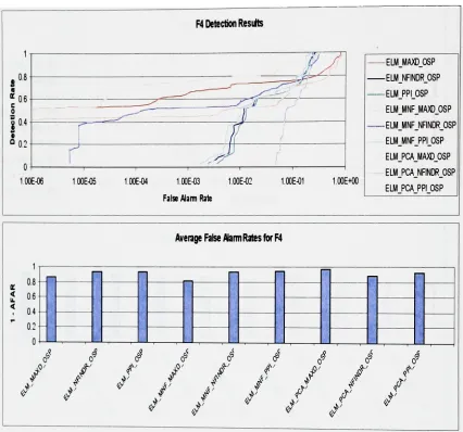
F4

target

56

7.5

1

AFAR

values

for

the

F13

target.

. .

56

7.6

1

AFAR

values

for

the

C5

target

56

7.7

1

AFAR

values

for

the

F8

target

57

7.8

1

AFAR

values

for

the

VF1

target

57

7.9

1

AFAR

values

for

the

VI

target

57

7.10 1

AFAR

values

for

the

VF6

target

58

7.11 Detection

rates at a

CFAR

of10-4

for

the

F3

target

59

7.12 Detection

rates at a

CFAR

of 10-4

for

the

F4

target

60

7.13 Detection

rates at a

CFAR

of 10~4

for

the

F13

target

60

7.14 Detection

rates at a

CFAR

of 10-4

for

the

C5

target

60

7.15 Detection

rates at a

CFAR

of 10~4

for

the

F8

target

61

7.16 Detection

rates at a

CFAR

of 10"4

for

the

VF1

target

61

7.17 Detection

rates at a

CFAR

of 10"4

for

the

VI

target

61

7.18 Detection

rates at a

CFAR

of 10"4

for

the

VF6

target

62

A.l

ROC

and

(1

-AFAR)

graphs

for

the

C5

target that

employed

the

ACORN

atmospheric compensation algorithm and

the

ASD

matched

filter

68

A.2

ROC

and

(1

-AFAR)

graphs

for

the

C5

target that

employed

the

ACORN

the

OSP

matched

filter

69

A.3

ROC

and

(1

-AFAR)

graphs

for

the

C5

target that

employed

the

ELM

(12)

LIST

OF FIGURES

A. 4

ROC

and

(1

-AFAR)

graphs

for

the

C5

target that

employed

the

ELM

the

OSP

matched

filter

71

A.5

ROC

and

(1

-AFAR)

graphs

for

the

C5

target

that

employed

the

FLAASH

the

ASD

matched

filter

72

A.6

ROC

and

(1

-AFAR)

graphs

for

the

C5

target that

employed

the

FLAASH

the

OSP

matched

filter

73

A.7

ROC

and

(1

-AFAR)

graphs

for

the

F3

target that

employed

the

ACORN

the

ASD

matched

filter

74

A.8

ROC

and

(1

-AFAR)

graphs

for

the

F3

target

that

employed

the

ACORN

atmosphericcompensation algorithm and

the

OSP

matched

filter

75

A.9

ROC

and

(1

-AFAR)

graphs

for

the

F3

target that

employed

the

ELM

atmospheric compensationalgorithm and

the

ASD

matched

filter

76

A. 10

ROC

and

(1

-AFAR)

graphs

for

the

F3 target

that

employed

the

ELM

the

OSP

matched

filter

77

A. 11

ROC

and

(1

-AFAR)

graphs

for

the

F3

target that

employed

the

FLAASH

the

ASD

matched

filter

78

A.12 ROC

and

(1

-AFAR)

graphs

for

the

F3

target

that

employed

the

FLAASH

the

OSP

matched

filter

79

A.13 ROC

and

(1

-AFAR)

graphs

for

the

F4

target that

employed

the

ACORN

atmospheric

compensation

algorithm and

the

ASD

matched

filter

80

A.14 ROC

and

(1

-AFAR)

graphs

for

the

F4

target that

employed

the

ACORN

atmospheric compensation algorithm

and

the

OSP

matched

filter

81

A.15ROC

and

(1

-AFAR)

graphs

for

the

F4 target that

employed

the

ELM

atmospheric compensation algorithm

and

the

ASD

matched

filter

82

A.16 ROC

and

(1

(13)

LIST OF FIGURES

A.

17

ROC

and

(1

-AFAR)

graphs

for

the

F4

target that

employed

the

FLAASH

atmospheric

compensation algorithm and

the

ASD

matched

filter

84

A.18 ROC

and

(1

-AFAR)

graphs

for the F4 target

that

employed

the

FLAASH

the

OSP

matched

filter

85

A.19 ROC

and

(1

-AFAR)

graphs

for

the

F8

target that

employed

the

ACORN

the

ASD

matched

filter

86

A.20 ROC

and

(1

-AFAR)

graphs

for

the

F8

target that

employed

the

ACORN

the

OSP

matched

filter

87

A.21 ROC

and

(1

-AFAR)

graphs

for

the

F8

target that

employed

the

ELM

the

ASD

matched

filter

88

A.22 ROC

and

(1

-AFAR)

graphs

for

the

F8

target that

employed

the

ELM

the

OSP

matched

filter

89

A.23 ROC

and

(1

-AFAR)

graphs

for

the

F8

target that

employed

the

FLAASH

the

ASD

matched

filter

90

A.24 ROC

and

(1

-AFAR)

graphs

for

the

F8

target that

employed

the

FLAASH

the

OSP

matched

filter

91

A.25

ROC

and

(1

-AFAR)

graphs

for

the

F13

target that

employed

the

ACORN

the

ASD

matched

filter

92

A.26 ROC

and

(1

-AFAR)

graphs

for

the

F13

target that

employed

the

ACORN

the

OSP

matched

filter

93

A.27

ROC

and

(1

-AFAR)

graphs

for

the

F13

target that

employed

the

ELM

the

ASD

matched

filter

94

A.28

ROC

and

(1

-AFAR)

graphs

for

the

F13

target

that

employed

the

ELM

atmospheric compensation algorithmand

the

OSP

matched

filter

95

A.29

ROC

and

(1

-AFAR)

graphs

for

the

F13

target that

employed

the

FLAASH

(14)

LIST

OF

FIGURES

A.30 ROC

and

(1

-AFAR)

graphs

for

the

F13

target that

employed

the

FLAASH

the

OSP

matched

filter

97

A.31 ROC

and

(1

-AFAR)

graphs

for

the

VI

target that

employed

the

ACORN

the

ASD

matched

filter

98

A.32 ROC

and

(1

-AFAR)

graphs

for

the

VI

target that

employed

the

ACORN

the

OSP

matched

filter

99

A.33 ROC

and

(1

-AFAR)

graphs

for

the

VI

target that

employed

the

ELM

the

ASD

matched

filter

100

A.34 ROC

and

(1

-AFAR)

graphs

for

the

VI

target that

employed

the

ELM

the

OSP

matched

filter

101

A.35

ROC

and

(1

-AFAR)

graphs

for

the

VI

target that

employed

the

FLAASH

the

ASD

matched

filter

102

A.36

ROC

and

(1

-AFAR)

graphs

for

the

VI

target

that

employed

the

FLAASH

the

OSP

matched

filter

103

A.37

ROC

and

(1

-AFAR)

graphs

for

the

VF1

target

that

employed

the

ACORN

the

ASD

matched

filter

104

A.38

ROC

and

(1

-AFAR)

graphs

for

the

VF1

target that

employed

the

ACORN

the

OSP

matched

filter

105

A.39

ROC

and

(1

-AFAR)

graphs

for

the

VF1

target that

employed

the

ELM

atmospheric _{compensation algorithm and}

the

ASD

_matched

filter

106

A.40 ROC

and

(1

-AFAR)

graphs

for

the

VF1

target that

employed

the

ELM

the

OSP

matched

filter

107

A.41

ROC

and

(1

-AFAR)

graphs

for

the

VF1

target that

employed

the

FLAASH

the

ASD

matched

filter

108

A.42

ROC

and

(1

-AFAR)

graphs

for

the

VF1

target

that

employed

the

FLAASH

(15)

10

LIST OF FIGURES

A.43 ROC

and

(1

-AFAR)

graphs

for

the

VF6

target that

employed

the

ACORN

the

ASD

matched

filter

110

A.44 ROC

and

(1

-AFAR)

graphs

for

the

VF6

target that

employed

the

ACORN

the

OSP

matched

filter

Ill

A.45 ROC

and

(1

-AFAR)

graphs

for

the

VF6

target that

employed

the

ELM

the

ASD

matched

filter

112

A.46

ROC

and

(1

-AFAR)

graphs

for

the

VF6

target that

employed

the

ELM

the

OSP

matched

filter

113

A.47 ROC

and

(1

-AFAR)

graphs

for

the

VF6

target that

employed

the

FLAASH

the

ASD

matched

filter

114

A.48

ROC

and

(1

-AFAR)

graphs

for

the

VF6

target that

employed

the

FLAASH

(16)

List

of

Tables

6.1

Table

ofselected

targets

44

6.2

Number

of

bands

and

total

percentage of

variability

retained after

PCA

was performedon

the

atmospherically

compensated

Forest Radiance I images

.

45

6.3

Number

of

bands

and

total

percentage of

variability

retained after

MNF

was performed on

the

atmospherically

compensated

Forest Radiance

I images

.

46

6.4

The

number of pixels considered and

the

number of endmembers selected

using PPI

for

each

image

48

6.5

The

number of endmembers

automatically

selected

by

N-FINDR for

each

image

50

7.1

Average (1

AFAR)

values

based

on atmospheric compensation algorithm.

63

7.2

Average (1

AFAR)

values

based

on

dimensionality/noise

reduction algo

rithm

for

chains

using ELM

63

7.3

Average (1

AFAR)

values

based

on

endmember

selection algorithm

for

chains

using ELM

and

PCA

64

7.4

Average (1

AFAR)

values

based

onmatched

filter

algorithm

for

chains

using

ELM, PCA,

and

N-FINDR

64

[image:16.525.66.477.214.571.2]

(17)

(18)

Chapter 1

Introduction

Detection

of

known

substances,

or

targets,

is

a

very

common problem

in hyperspectral

imaging

(HSI). Given

a

target

with a

known

spectral

signature,

an algorithm

that

can

decide if

and where

that

target

is

present

in

an

image is

needed.

In

order

to

accomplish

this,

target

detection

algorithms such as matched

filters

have been developed

to

accentuate

pixels

in

an

image

that

contain

the target.

HSI

can

be

thought

of as

taking

an

image

of

the

same scene with numerous

(normally

hundreds)

different

spectral

bands. At

each

pixel,

a spectrum measuredrepresents

the

op

tical energy

versus wavelength.

These

spectra are

pictorially displayed

as a

third

dimension

in

Figure 1.1. Each layer in

the

cuberepresents aspectral

band;

every band

containssimilar

spatial

information.

There

are several unique steps

to

any

target

detection

algorithm chain.

Each

of

these

stepsplays a role

in

determining

the

overall performanceof

the target

detector. Figure

1.2

is

a

flow

chart

detailing

each of

the

more significant steps

for

a generic

target

detection

algorithm chain.

For

each

individual step along

the way, there

_{are several algorithms}

that

will return an acceptable solution.

It is

desired

to

determine

the

best

algorithm

to

accom

plish each step.

A

particular

combination

of

algorithms

may

work well

for

one

image

or

target

but

may

also perform

terribly

for

a

different image

_or

target.

Finding

_an

optimal

(19)

i_^

Chapter!

.

Introduction

combination of algorithms or recipe

becomes

an

intriguing

dilemma.

In

order

to

best

accomplish

this,

commonly

used

algorithms

for

each

step

must

be

looked

at and compared

to

eachother

for

many

different

types

of

targets

in

an

image. Each

of

the

steps

in

the

chain

performs a

distinct

and

important

role

in

the

overall

target detection

process.

Known

target

spectra are

in

units of

reflectance,

since

that

is

what

is

able

to

be

measured

in

a

lab

or

in

the

field.

The data

collected

remotely

by

a sensor

is in

units of radiance.

The

difference

between

these

measurements

is

the

atmosphere

between

the

remote sensor and

the target.

If

the

atmospherewas able

to

be effectively

"removed"

,

the

collected

information

would

be

in

the

sameunits as

the

measured

information. This is

what

the

step

seeks

to

accomplish.

Hyperspectral

sensors

generally

collect

hundreds

of

bands

worth of

information.

This

amount of

data

can

be

very

computationally

cumbersome or even

impossible

to

work with.

The

dimensionality

reduction

step

seeks

to

decrease

the

amount of

data

on which

to

operate

without

removing any

pertinent

information.

Noise is

a

very

common problem with

any

sensor.

Noise

can

be

removed

simultaneously

with other

unnecessary

information.

Because

of

this,

the

noise and

dimensionality

reduction steps are often performed

together.

One

way to

describe

the

background

of an

image is

structured,

or geometrically.

That

(20)

15

is

to

say that

a set of

basis

vectors

is

used

to

describe

the background.

These basis

vectors

are referred

to

asendmembers.

The

endmemberselection

step

determines

that

set of

basis

vectors.

Finally,

the

matched

filters

are

the

mathematical operations

that

determine the

likelihood

that

aspecific pixelcontains a

known

target

spectrum.

The

following

chapters

discuss,

in

detail,

the

background

and

theoretical

explanation

of

the

algorithms studied

in

this

effort.

Results

are presented

in

the

form

of

ROC

curves,

average

false

alarm rates

(AFAR)

(Bajorski

et

al.,

2004),

and

detection

rates at aconstant

(21)

16

ChapterI.

Introduction

Image

Dimensionality

/ Noise

Reduction

Preprocessed

Image

Known Target

Reflectance

Vector

Background Characterization

Endmember Selection

Covariance Calculation

Target Detection

Algorithm

Structured

Background

Matched Filter

Unstructured Background

Matched Filter

Target

Abundance

Map

(22)

Chapter

2

Atmospheric

compensation

is

the

process of

"removing"

the

illumination

and atmosphere

from

the

image.

Often,

the

known

spectral signature ofa

target

consists of reflectance val

ues measured

in

a

lab. These

measurements cannot

take

into

account

the

effects of

looking

through

thousands

of

feet

of atmosphere.

The

ultimate goal of

the

atmospheric compensa

tion

process

is

to

retrieve surface reflectance values

from

the

radiance values recorded

by

the

sensor.

Equation 2.1 is

one version of

the

sensor

reaching

radiance equation

(ignoring

thermal

radiance)

presented

by

Schott

(Schott,

1997):

Lx

=

[E'sX

cosa'nixf-^-

+

FEdsXT-^-

+

(1

-F)LbsXrd{X)]r2

+

LusX

(2.1)

where

E'sX

is

the

top

ofatmosphere solar

irradiance,

a'

is

the

solar

declination

angle

from

the target

centered z

axis, n

is

the

atmospheric

transmission

of

the

path

from

the

sun

to

the

target,

r

is

the

reflectance, F is

the

fraction

of

the

hemisphere

above

the target that

is

unobstructed

(sky),

E^

is

the

downwelled

irradiance,

rd

is

the

diffuse

reflectance,

Lbs

is

the

reflected

background

radiance,

r2

is

the

atmospheric

transmission

of

the

path

from

the

target to the

sensor,

Lus

is

the

upwelled

radiance,

and

A

denotes

the

wavelength

dependency

of

the

associated

terms.

The

terms

in

Equation

2.1

that the

atmosphere

directly

contributes

to

are

the two

path

transmittance

terms,

n

_and _r2.

As

_can

be

seen, these two

terms

-r2

(23)

I8.

Chapter2.

Atmospheric

Compensation

in

particular - _will

have

_a

significant

effect on

the

overallsensor

reaching

radiance.

All

of

the

factors

that

determine

the

atmosphere- _water

vapor,

molecular

constituents,

atmospheric

density,

etc. can

substantially

_alter

the

way

the

same

target

looks

under

different

conditions.

As

a

result, the

atmosphere

through

which an

image

was

taken

must

be determined

and

taken

into

account.

The

simplest

form

of atmospheric compensation

is

the

Empirical Line

Method

(ELM). There

are several other algorithms

that

make use of

atmospheric

inversion

principles:

the

Fast

Line-of-Sight Atmospheric Analysis

of

Spectral

Hypercubes

(FLAASH)

and

Atmospheric CORrection

Now

(ACORN)

are

two

of

the

more

widely

used atmospheric

inversion

based

algorithms.

These

three

methods are used

in

this

work and will

be discussed here.

2.1

Empirical Line Method

(ELM)

ELM

relies on ground

truth

inasmuch

as at

least

two

different

regions

in

the

image

(preferably

one

dark

and one

light

across each

wavelength) have

a

known

reflectivity.

These

regions must

be

at

least

one

fully

resolved pixel

large. In

order

to

ensure

that

an

uncontami-nated,

fully

resolved pixel

is

available, these

regions

generally have

to

be

several pixels

large

in

each

direction.

The

regions must

have

corresponding

ground

truth

reflectance

spectra,

ideally

taken

at

the

same

time

as

the

image.

If

such regions are not present

in

the

image,

an educatedguess can

be

made

by

selection of regions

for

whichan approximate reflectance

can

be

created.

For

example,

a white cloud

may

have

a

reflectivity

of about

90%

across

all wavelengths.

Obviously,

there

is

a great

opportunity

for

error

introduction if

estimates

have

to

be

made,

but

that

can

be limited if

they

are made smartly.

Once

the two

(or

more)

regions

have been

selected,

a

line is

fit

through the

radiance

(or

digital

counts)

vs

reflectivity

points

in

each

band. ELM

assumes a

linear

relationship

be

tween the

radiance

(or

digital counts)

and

the

reflectivity.

Mathematically,

this relationship

(24)

2.2.

19

L(X)

=

m(A)

*

r(A) +

6(A)

(2.2)

where

L is

the

observed radiance

(or

digital

count),

m

is

the

slope of

the

line

through

the

ground

truth

points,

r

is

the reflectance,

and

b

is

the

radiance

(or

digital count)

value

that

represents zero reflectance.

All

of

the terms

have

a wavelength

dependency,

A.

Equation

2.2 is

a

very

simplified

linear

version of

Equation 2.1.

Figure 2.1 illustrates

this

linear

relationship

graphically.

P

/

r c

f

TO

/

D "0

/

as

'

1

I

/

Reflectance

BandX

BandY

Figure

2.1:

Graphical

representation of

ELM for

two

bands.

The

marked points are

the

"ground

truth"

points.

Now,

the

observed radiance

in every

pixel

in

the

image

can

be

converted

into

reflectance

using the

linear

regression coefficients

(m

and

b)

obtained via

Equation 2.2. It is important

to

note

that

ELM

can work with

both

radiance or

digital

counts without calibration.

2.2

An

alternative method

to

ELM for

calculation of atmospheric effects on an

image

is

to

characterize

the

atmosphere

in

an

image

to

make "removal" possible.

There

are

three

main

factors

that,

once

determined,

can

adequately

characterize

the

_atmosphere: _optical

depth

of

the

different

aerosol and molecular

constituents,

surface pressure

elevation,

and

(25)

20

Chapter2. Atmospheric

Compensation

Atmospheric

inversion

exploits

the

unique absorption

features

of

the varying

atmo

spheric materials at

different

wavelengths

in

order

to

arrive at

the

optical

depth for

the

various aerosols present

in

the

atmosphere.

Figure

2.2

shows

the

absorption spectra

for

some common atmospheric molecularconstituents.

The

strength,

or

depth,

of

these

unique

features

is

used

to

determine

the

quantity

of

the

specific molecular constituent

in

the

at

mosphere.

1

v

Y~*

50

0

1

2

3

4

5

6

?!

3

13

11

12

13

M

Wavelength

(um)

0

1

2

3

4

5

8

7

I

9

13

11

12

13 14

Wavelength (|imi

c

*

V

0

*

CO

i

50

s

t *

<1

i r

: r ,

1 , L

0

1

2

J

4

5

S

T

t

9

10

11

12 13

14

Wavelength

(urn)

1

2

3

4

S

7

8

J

10 11 12

14

Wavelength

(|im)

3

1

I

3

4

i

6

1

I

%

11 11

13

Wavelength

(pm)

0

1

2

3

4

5

S

T

I

3

10

11

12

13

14

Wavelength

(urn)

Figure 2.2: Absorption

spectra of several common molecular constituents

in

the

atmosphere

(Schott,

1997).

The

second

factor

that

needs

to

be determined is

the

surface pressure elevation.

This

allows

for

compensation of atmospheric absorption

due

to

well mixed gases

in

the

atmo

sphere and

the

effects ofmolecular

scattering

(Green

et

al., 1993).

The

amount of oxygen

is

agood

indicator

of pressure

depth. Oxygen

can

be

treated

the

sameas

any

other

(26)

atmo-2.2.

Atmospheric

Inversion

21

spheric molecular

constituent,

and so

the

process

for

calculating

the

quantity

of oxygen

is

the

same as

for

the

other molecularconstituents.

The

absorption

feature

of oxygen present

at w

760nm is

most

commonly

used

in

this

process.

The third,

and perhapsmost

important,

contributor

to

atmospheric characterization

is

water vapor.

The

absorption spectrum

for

water

is

given

in

Figure 2.3.

The

absorption

feature

present at

940nm is commonly

used

to

determine

the

amount of water vapor

present

in

the

atmosphere.

There

are also

strong

features

at ss

1120nm

and

1340nm that

could also

be

used.

w*r*#vpoiAbsorptionSp*tr

Figure 2.3:

Absorption

spectrumofwater.

Simulation

is

used

heavily

in this

process.

MODTRAN (Berk

_et

al.,

2005)

is commonly

utilized

to

model

the

absorption

features for

many

different

concentrations

of

the

varying

aerosols

in

the

atmosphere.

These

simulated absorption

features

are

compared

to the

ob

served

feature

and

the

closest match

determines

the

concentration

_of

the

aerosols present

in

the

atmosphereof

the

given

image.

The

non-linear

least

squared spectral

fit

(NLLSSF)

algorithm

(Green

et

al.,

1993)

is

the

primary

determining

_metric

for

matching the

modeled

(27)

^2

Chapter2. Atmospheric Compensation

2.2.1

Fast Line-of-Sight

Atmospheric

Analysis

of

Spectral

Hypercubes

(FLAASH)

FLAASH is

a

commercially

available atmospheric

compensation algorithm

developed

by

the

Air Force Research

Laboratory,

Space Vehicles Directorate

(AFRL/VS)

to

support

the

analysis of visible

to

shortwave

infrared

(0.4

urn

to

2Aum)

hyperspectral

and

mul-tispectral

sensors

(Berk

et

al., 2002).

Using

the

atmospheric

inversion

method

described

above,

FLAASH is

able

to

determine

the

aerosol and water vapor content of

the

atmo

sphere

in

an

image

as well as

the

surface pressure.

FLAASH

was

designed

as a general

purpose code

developed

in

parallel with upgrades

to

MODTRAN.

Originally,

FLAASH

was

designed

to

work with

MODTRAN4. Because

of

this

"side-by-side"

development

and

up

grade,

FLAASH is

able

to

exploit

the

speed gains and

accuracy

improvements

obtained

by

ongoing improvements

to

MODTRAN.

Another

feature

present

in

FLAASH,

whichwill

not

be discussed

in

detail,

is

the

ability

to

effectively

remove clouds

from

an

image.

This

is

done

by identifying

cloud pixels

in

the

image

and

replacing them

with average radiance

values of

the

pixels

surrounding

the

cloud.

Equation 2.3

(Berk

et

al.,

2002)

is

the

sensor

reaching

radiance

(L*)

equation utilized

by

FLAASH

that

has

a

different form

than

Equation 2.1

but

will return

the

same value:

L*

=

-^-+

-^

+

Ll

(2.3)

1

-peb

1

-peb

where

p is

the

pixel surface reflectance

(equivalent

to

r

in

Equation

2.1),

pe

is

an average

surface reflectance

for

the

area

surrounding the

pixel

in

question,

S

is

the

spherical albedo

of

the

atmosphere

(accounting

for

the

skylight

photons),

L*

is

the

upwelled

radiance,

A

and

B

are surface

independent

coefficients

that vary

based

on

the

atmospheric and geometric

conditions.

All

of

the

variables are

implicitly

wavelength

dependent.

The

pe

is included

to

allow

FLAASH

to take

into

account

the

adjacency

effects of

the surrounding

pixels on

the

pixel

in

question.

(28)

2.2.

Atmospheric

Inversion

23

Once

these

values

have

been

extracted,

Equation 2.4

is

used

to

solve

for

pe

(Berk

et

al.,

2002):

L.=

(AB)^

+

K

(24)

i peJ

where L*

is

a

spatially

averagedsensor

reaching

radiance value.

Once

pe

has

been

determined,

Equation 2.3

can

be

solved

for

reflectance

(p).

2.2.2

Atmospheric CORrection Now

(ACORN)

Like

FLAASH,

ACORN is

an atmospheric compensation algorithm

that

can model

aerosol absorption

in

the

atmosphere

based

on

look-up-tables

that

are produced

using

MODTRAN4.

However,

this

algorithm

is

capable of

determining

both

molecular andaerosol

scattering

effects aswell.

The

equation utilized

by

ACORN

to

represent

the

sensor

reaching

radiance

is

Equation 2.5

(ImSpec, 2004)

:

MA)

=

Fo(A)

TT

Td(X)p(X)Tu(X)

Pa(A)

+

(2.5)

(1

-s(X)p(X))

J

where

Lt

is

the total

sensor

reaching

radiance,

Fo

is

the

above atmospheresolar

irradiance,

Td

and

Tu

are

the

downward

and upward

transmittance

of

the

atmosphere,

pa

and s are

the

upward and

downward

atmospheric

reflectance, p

is

the

surface spectral reflectance and

A

denotes

the

wavelength

dependency

of

the

associated

terms.

ACORN

seeks

to

solve

Equation 2.5 for

the

surface reflectance value of each

pixel,

p.

This

solution

is

given

in

Equation 2.6

(ImSpec, 2004)

:

p(X)

=

F0(X)Td(X)Tu(X)

+ S(X)

-1

(2.6)

_Lt(X) -

MhkziV

A

key

unique

feature

of

the

ACORN

algorithm

is

full

spectral

fitting

to

solve

for

the

overlap

of absorption

due

to

water vapor and

liquid

water

in

surface vegetation

(Kruse,

2004).

The

outputsof

this

_{software package are a water vapor}

image

_{and a scaled} _surface

reflectance cube.

ACORN

is commercially

available

_and

is

distributed

(29)

24

Chapter2. Atmospheric Compensation

2.3

Discussion

In

this

chapter,

three

different,

valid atmospheric compensation

techniques

are pre

sented.

All

three

accomplish

the

same

task,

but

there

are

inherent

differences in

the

output

of eachalgorithm.

There

are some similarities

between

the way

FLAASH

accomplishes

this

and

the

way

ACORN

does,

but

they

are still quite

different from

each other.

The

major

differences

are

the

assumptionseach algorithm makesand

the

complexity

of

its

mathemat

ical

operations.

ACORN

is essentially

a simpler version of

FLAASH. FLAASH

takes

into

account

the

adjacency

effectsof

neighboring

pixels

in its

calculation of surface

reflectance,

while

ACORN

does

not

have

this

feature.

This

alonewill cause

the

outputs

to

be

radically

different

from

each other.

The governing

equations

for FLAASH

(Equations

2.3

and

2.4)

and

ACORN

(Equations

2.5

and

2.6)

are

obviously

not

the

same.

Again,

this

introduces dif

ferences

in

the

outputsof

the

algorithms.

Finally,

both FLAASH

and

ACORN

differ greatly

from

ELM

which assumes a

linear

relationship

between

the

radiance values collected and

surface reflectance.

Of

all

the

steps

looked

at

in

this research, the

step

should

have

the

greatest effect on

the

overall

target

detection

performance.

This is

expected

because

this

step

actually

changes

the

values present

in

the image.

Also,

this

is

the

first

step

in

the chain,

so

any

errors

introduced

in

this

step

will

be

amplified and can

potentially

(30)

Chapter

3

Dimensionality/Noise Reduction

The

next steps

in

the target

detection

process are

dimensionality

reduction and noise

reduction.

Since

these

two topics

are

closely related, the

background for

them

both

can

be

discussed

simultaneously.

Many

algorithms

tackle

both

problems at

the

same

time.

The

need

for

noise reduction

is

fairly

obvious;

as with

any image

processing,

noise

interferes

with

the

actual signal.

It is

because

of

this

interference

that the

noise should

be

reduced

(ideally

eliminated) before

any

processing is

done

on an

image.

The

need

for

dimensionality

reduction

may

not

be

as

intuitive

as noise reduction.

As

mentioned

in

Chapter

1,

HSI

relies on

up to

hundreds

of spectral

bands

of

information.

Using

all of

the

information

contained

in

all of

these

bands

can

lead

to

dauntingly

large

data

sets

that may

be computationally

difficult

or

impossible

to

manage.

Images

willcontain

varying

amounts

of pertinent

information in

some

bands

while

carrying

little

or no significant

information

in

others.

Also,

it is

likely

that there

is

some

information

that

is

redundant across several

bands

and

therefore

can

be

reduced

by discarding

the

repeated

instances.

This

can

be

exploited,

and

the

bands

containing

little

amounts of

data

can

be discarded

reducing

the

amount of

information

to

be

operated on

to

a manageable

level.

(31)

2_^

Chapter3. Dimensionality/Noise Reduction

3.1

Principal Components Analysis

(PCA)

Perhaps

the

most common

method

of

dimensionality

reduction

is

Principal

Components

Analysis (PCA). A

common

assumption

associated with

PCA is

that

variability

equals

information.

Because

of

this,

bands

with

high

variancewill

dominate

the

first few

principal

components.

Conversely,

bands

with

low

variance

that

may

still contain useful

information

will

be

mixed

in

withnoise

from

the

more

varying bands.

As

is

implied

by

the name,

PCA breaks down

the

data into its

principal components.

In

order

to

do

this,

the

covariance matrix

for

the

data

must

be

constructed.

The

covariance

matrix

describes

the

dependant

variability

of

the

bands

with relation

to

each other.

Once

the

covariancematrix

has

been

determined,

its

eigenvectorscan

be

calculated.

These

orthogonal

eigenvectors areused

to

rotate

the

original

data into

anew space

that

exactly de-correlates

the

data.

For

the

most

part, the

first few

principal component

bands

contain

the majority

of

the

variability in

an

image. Because

of

this,

PCA

can

be

used

to

greatly

reduce

the

number of

dimensions

on which

to

operate

by disregarding

the

lower PCA bands. Figure 3.1

shows a

simple example of

PCA

performed on a six

band

scene of

Rochester,

NY

where

the

six

PCA

bands

are

displayed.

There is

no "right"

way

of

determining

the

number of

PCA

bands

to

keep

for

an

image.

The

amount of variation maintained must

be

weighed against

the

computational

complexity

of

keeping

a number of

PCA bands. For

the

example

in Figure

3.1,

if only

the

first four

bands

were

kept,

99.33%

of

the variability

is

maintained.

This

is

enough

to

effectively

reduce

the

dimensionality

without

greatly altering

the

amount of

information

on which

to

operate.

3.2

Maximum

Noise Fraction

(MNF)

A

second algorithm

that

reduces

dimensionality,

the

Maximum

Noise

Fraction

(MNF)

(32)

3.2.

Maximum

Xoise Fraction

(MNF)

27

(5S

55)

(7

28)

(32

54)

(0.59)

(0

03)

Figure 3.1: Principal

component

images from

asix

band

image

of

Rochester,

NY. Percentage

(33)

28

Chapter3. Dimensionality/Noise

Reduction

Essentially,

the

MNF

algorithm

is the

same as

the

PCA

processwith some "pre-processing"

steps added.

For the MNF

transform,

the

covariance matrixof

the

noisepresent

is

needed.

One

way to

obtain

this

in-scene

(if

it is

not

known)

is

by locating

a

radiometrically

flat

field. Once

a

flat field

is

identified

within an

image,

the

mean can

be

subtracted

from

the

observed valuesof

that

field. The

result

is

arepresentationof

the

noisepresent

in

the

image.

Once

this

"noise

image"

is

found,

its

covariance matrix can

be

calculated.

The

this

process

is

basically

to

perform

PCA

on

the

noise

image

to

de-correlate

the

noise.

This is

done

by

calculating

the

eigenvectors of

the

noise

image.

By

definition,

the

resulting

eigenvectors are orthogonal

to

each other.

The

original

image

can

now

be "passed

through"

this

orthogonal

transformation.

After

this

is

done,

the

orthog

onally

transformed

image

can

be

whitened,

or

normalized,

by

the

eigenvalues of

the

noise

covariance matrix.

The

final

result of all

these

steps

is

an

image in

which all of

the

noise

present

is

orthogonal and

identical.

Now,

the

PCA previously described

can

be

performed.

The

advantage of

the

MNF

transform

is

that the

"pre-processing"

steps

force

the

as

sumption used

in PCA

of variance

representing information

to

be

true.

There is

now equal

variance present

due

to

noise

in

the

image.

The bands

are rank ordered

by

the

signal

to

noise

ratios and

the

highest PC bands

are retained.

The

result

is

a

greatly

reduced

dimension

spacewith

little

noise

to

interfere

with

target

detection.

3.3

Discussion

As

described

above, the

process

involved in both PCA

and

MNF is

very similar,

however,

the

results will

be

dramatically

different.

This difference

stems

from

the

fact

that

MNF

uses

the

eigenvectors

from

a

different

matrix

to

perform

the

rotation

in

aneffort

to

reduce noise.

Calculation

of

the

eigenvectors and

the

actual rotations are rather

trivial

mathematical

operations.

Neither PCA

nor

MNF

change

the

amount of

information

present

in

the

data.

However,

in

order

to

reduce

dimensionality,

some of

the

lower

components

have

to

be

thrown

(34)

3.3.

Discussion

29

removed

is

noise

(as

is

the

goal of

MNF),

the

overall performance of

the

algorithm chain

can

improve.

Conversely,

if

the

removed

PC

bands

contain some pertinent

data,

the

overall

performanceof

the

algorithm chain can

be

greatly

degraded.

If

the

noise

image"

does

not characterize

the

noise present

in

the

image

well,

the

eigenvectors

derived

will not rotate

the

data into

a space

that

is

orthogonal

to the true

noise

in

the

image.

What

willend

up

happening

is

the

data

will

be

rotated

into

a space

that

is

orthogonal

to

some of

the

pertinent

information

causing

poor

information

to

be

passed on

to the

in

the

chain.

Another

situation

that

will

hinder

the

ability

of

MNF

to

improve

the

overall algorithm

chain,

is

there

being

very

little

noise

in

an

image

to

begin

with.

Extremely

low

noise

is

very

difficult

to

characterize well.

The

algorithm

for

this step that

is

expected

to

most

greatly improve

the

detection

results

is

the

"none" case.

This is due

to the

fact

that

no

information is

being

removed

from

the

original

image.

By

performing PCA

or

MNF,

that

sheer amount of

data is

reduced

to

a

point where

it is

much moremanageablecomputationally.

Clearly,

there

is

a

trade

off

here,

however

this

aspect will not

be

discussed

in

detail in

this

research.

The

focus

is solely

on

(35)

(36)

Chapter

4

Endmember Selection

There

are

two

overarching

ways

to

characterize

the

background

of an

image:

structured

or unstructured.

A

structured

background

is

one

that

is

defined

by

a set of

basis

vectors.

This

set of

basis

vectors,

or

endmembers,

completely defines every

non-target pixel

in

an

image,

in

theory.

An

unstructured

background

is

defined

statistically, normally

by

a covari

ance or correlation matrix.

While

a

background independent

matched

filter,

the

Spectral

Angle Mapper

(SAM),

and an unstructured matched

filter,

the

generalized

likelihood

ratio

test

(GLRT),

were used

in

determining

the

targets,

this

research

focuses

on matched

filters

that employ

astructured

background.

All

targets

fall into

two very

broad

categories: resolved and unresolved.

A

fully

resolved

target

is

one

that

fills

at

least

one entire pixel

in

an

image.

An

unresolved

target

is

one

that

does

not

fully

fill

a pixel.

For

targets that

are

unresolved, it

becomes

necessary

to

determine

the

constituents of each pixel when

using

a

structured

background

model.

In

order

to

accomplish

this,

each pixelmust

be

represented asacombinationof

its

components

(or

endmembers).

A

common

representation,

known

as

the

linear

mixing

model

(LMM),

for

a mixed pixel

is

shown

in

Equation

4.1:

L

=

EF

(4.1)

(37)

32

Chapter4.

Endmember

Selection

where

L is the

radiancevectorof

the pixel, E is

the

endmember

matrix,

and

F is

the

vector

ofunknown endmember

fractions. This

representation

is

based

on

the

assumption

that

each

pixel

is

a

linear

combination of

the

image

endmembers.

Every

pixel

in

an

image,

whether

it

contains

target

or

not,

can

be

represented

using

the

LMM.

However,

the accuracy

is

determined

by

how

well

the

set of endmembers characterizes

the

scene.

In

order

to

enable

the

matched

filters

to

properly

suppress

the

background in

an

im

age, the

background

must

first

be

wellcharacterized.

This is

accomplished

by

deriving

the

endmembersused

to

define

the

background

pixels.

In

theory,

the

background is

fully

char

acterized

by

a matrix

consisting

of all

the

endmembers

that

mix

to

define

all non-target

signals present

in

the

image.

This

would represent an

ideal

situation

that

would result

in

endmember matrices

that

could

be

almost as

large

as

the

image itself

and

rendering the

matched

filters

nearly

too

computationally

cumbersome

to

use.

In

practice,

several

end-members are used

to

represent

the

entire

background. There

are several

different

methods

of

eliciting

these

endmembers

directly

from

an

image,

three

will

be discussed here:

PPI,

MAXD,

and

N-FINDR.

4.1

Pixel

Purity

Index

(PPI)

The first

endmember selection algorithm

is

the

Pixel

Purity

Index

(PPI)

method

(Board-manet

al, 1995).

Using PPI,

all of

the

pixel values

in

an

image

are projected onto

randomly

selected vectors.

Each

time

a projection

is

accomplished,

the

extreme points are noted.

Spectrally

pure pixels will

consistently

be

extreme points of

these

random projections.

A

major assumption of

this

method

is

that spectrally

pure pixels

(which

are

endmembers)

are present

in

the image.

This is

generally

a good assumption.

This

method

is

also rather

susceptible

to noise,

so steps

{e.g.

thresholding)

should

be

taken to

help

lessen

the

negative

(38)

4.2.

MAXD

33

4.2

MAXD

The

second endmember selection

technique

is MAXD

(Lee,

2004).

Similar

to

PPI,

MAXD

also uses projection

to

help

sort out

the

endmembers of an

image.

Given

a set of

data

points,

MAXD begins

by

selecting the

points

that

have

the

maximum and minimum

Euclidean

distance from

the

origin.

These

two

points are

the

first

two

endmembers.

Once

these

points are

selected,

all of

the

data

points are projected onto a vector orthogonal

to

the

difference

vector

between

the

first two,

and

the

pixel

the

maximum

distance from

the

common point projection of

the

first

two

is

selectedas

the

next endmember.

This

process

is

repeated until

the

desired

number of endmembers

is found. Figure 4.2

pictorially

explains

how

this

process works.

4.3

N-FINDR

Another

method of

determining

endmembers

in

an

image is

N-FINDR

(Winter,

1999).

This

method again

looks for

extrema points

in

the

data

set.

The

set of

data

points

for

an

image in

N-dimensional

space can

be

thought

of as a

convex-hull,

where one more

o

CO

,

BandX

(39)

34

Chapter4.

Endmember Selection

endmember

than

dimensions

is

needed

to

make aclosed convex

hull. For

example,

given an

image

with

two

bands

(dimensions),

three

endmembers

form

a

triangle

as a closed convex

hull

(Figure

4.3).

This

algorithm was

originally

packaged

for

use

in

unmixing

pixels

in

an

image

as opposed

to target

detection.

However,

both

processes require endmembers

to

be

elicited

from

the

image

first. Because

of

this overlap,

N-FINDR is

able

to

be

used

for

background

characterization

due

to

its ability

to

return

the

spectra of all

the

endmembers

it

uses

to

unmix an

image.

N-FINDR

assumes

that

spectrally

pure pixels can represent endmembers.

Clusters

of

[

.anto-tctisiaiitc

/

*

,^.

.

.Smallest

distance

'

\

ft K

Figure 4.2: MAXD

endmember selection algorithm

(Lee,

2004).

3

2

.

BandX

(40)

4.3.

X-FINDR

35

pixelsaround

the

areaofa "point" on

the

convex

hull,

suchas

the

clusters

labeled

1,

2,

and

3 in Figure

4.3,

are

indications

of

spectrally

pure pixels.

Spectrally

mixed pixels

generally

appear

between

the

pure

pixels,

sometimes outside of

the

convex

hull,

and are recognized as non-endmembers

by

N-FINDR.

As

a

starting

point,

N-FINDR

randomly

selects a

group

of pixels

(automatically

deter

mined

by

a statistical analysis of

the

image

(Senna

Consulting,

2004))

so

that

a convex

hull

can

be formed.

Once

these

points

have

been chosen,

the

volume of

the

convex

hull

is

computed.

This

is

repeated until

every

possible combination of points

that

could

form

a

convex

hull has been

used and

has

a volume associated with

it.

The

set of points

resulting

in

the

largest

volume

is

then

selected as

the

end members.

Figure 4.4 graphically

shows

the

maximum volume convex

hull

selected

for

a

two

band image.

c

CO

CD

Endmember b

Endmember

a

Shade

point

Band

Figure

4.4:

Maximum

volume convex

hull

for

a

two

band image

(Senna

Consulting,

2004).

This

algorithm

is

also

very

sensitive

to

noise.

So,

as with

PPI

and

MAXD,

steps need

(41)

36

Chapter4. Endmember Selection

4.4

Discussion

The

ultimate goal of

this step in the

algorithm chain

is

to

characterize

the

background

of

an

image

by determining

aset a

basis

vectors representativeof

the

background.

All

three

of

Comparison of Hyperspectral Imagery Target Detection Algorithm Chains

Rochester Institute of Technology

in Theses by an authorized administrator of RIT Scholar Works. For more information, please contact

in the

)'f.S. Degree

David Messinger

Memorial

Chains

involved in

filtering

background

Spectral Hypercubes

CONTENTS

Algorithm Chain Evaluation

(Schott,

background

target

target

target

target that

filter

target

filter

target that

filter

target that

filter

target that

filter

target that

filter

target that

FLAASH

filter

target that

filter

target that

FLAASH

automatically

ELM, PCA,

thought

determining

combination

different

the target.

Noise is

determines

detection

Target

Equation 2.1 is

hemisphere

terms

substantially

Hypercubes

known

example,

linear

the terms

using the

Atmospheric

0

Wavelength

0

0

0

Atmospheric

There

feature

Atmospheric

image

image.

surrounding the

Atmospheric

using

dependency

Chapter2. Atmospheric Compensation

differences

(Equations

target

Since