Resolvent Analysis and Data-Assimilation
Thesis by
Sean Pearson Symon
In Partial Fulfillment of the Requirements for the degree of
Ph.D. Aeronautics
CALIFORNIA INSTITUTE OF TECHNOLOGY
Pasadena, California
2018
© 2018
SeanPearsonSymon
ORCID: 0000-0001-9085-0778
ACKNOWLEDGEMENTS
First I would like to thank my family, particularly my parents who decided to leave
their friends and family behind in Scotland for a new life in the U.S. This was such
a brave decision on their part, particularly since my sister and I were only two and
four years old, respectively, at the time. I cannot overstate the number of doors that
have been opened for me as a result of their decision. My family in Scotland has also been incredibly supportive and it always feels like paradise when I can leave
behind my world here and fly across the ocean to see them.
Next, I would like to thank my thesis committee: Professors Tim Colonius,
An-thony Leonard, and Dan Meiron. Each member of my committee has helped me
much more than they probably think they have by asking insightful questions during
conferences/presentations or offering seemingly simple advice which turned out to
be incredibly useful. I next would like to thank my fellow G1’s especially Mélanie
Delapierre, Simon Lapointe, Neel Nadkarni, Chris Roh, and Kevin Rosenberg. I think every GALCIT student appreciates that the friendship you develop with your
fellow first years is quite special as most grad students don’t have to take on five
classes as soon as they arrive at Caltech. My choice to study abroad at Ecole
Poly-technique meant that I took quals a year later than everyone else. My fellow G2’s,
as I like to call them, were extremely welcoming when I returned from France,
par-ticularly Noah Braun, Ian Brownstein, Ilana Gat, David & Nikki Huynh, and Jason
& Susie Schlup. Quals were not the most pleasant experience for me but I was able
to get through them largely in part due to their help.
There are several more GALCIT individuals who I would like to mention. First and
foremost is Christine Ramirez, who was my first point of contact with Caltech. She
has always been incredibly helpful and welcoming to not only me but also the rest of
the incoming class. I would like to thank both Dimity Nelson and Peggy Blue, the
department administrators, for their incredibly efficiency with running GALCIT.
With respect to the faculty, I would like to acknowledge Ravi, who I met during
visit day. His personality impressed me so much that it ended up being one of the
primary reasons I chose to attend Caltech. I would also like to thank Professors
Pullin and Dimotakis, who taught Ae101. Despite having very different teaching styles, I learned a significant amount in this course and it fundamentally changed
my perspectives and approach to science. It was also nice to go full circle and TA
I also thank GALCIT for allowing me to participate in the Ecole Polytechnique
exchange program, where I met my friends Charu Datt and Keshav Raja. I still
enjoy talking about politics and science on a regular basis with Keshav. During my research internship at ESPCI, I had the very good fortune of being paired up with
my mentor, Anaïs Gauthier. As an inexperienced scientist, I learned a great deal
from her and other members of the lab directed by David Quéré and Christophe
Clanet. This brings me finally to my advisor in France, David Quéré, who I would
like to thank for allowing me to join the group based exclusively on my enthusiasm
for the projects in his lab.
I would like to thank my collaborators Rémi Carmigniani, Peter Schmid, and Denis
Sipp. Rémi was one of my fellow first years and teammate for Ae104c along with Simon Lapointe for the bouncing oil drops experiment. It was a great pleasure to
work with both of them on this project although it took months for me to finally
convince myself that my hands were rid of all traces of the silicone oil we used! I
met Peter briefly before I headed over to France as he was on sabbatical and spent
some of his time at Caltech. Peter has been an incredibly positive influence on my
Ph.D. in a number of ways including the control of shear flows course he taught at
Polytechnique and our collaboration on the experimental data-assimilation project.
He also co-organized a workshop in the heart of Tuscany where I met Denis, who
also played a very positive role on my Ph.D. research both in terms of the data-assimilation project as well as resolvent analysis. I wish to thank him in particular
for making his codes available at the workshop and assisting me with setting up the
resolvent code on a Caltech cluster.
There are some friends outside of research who I would like to thank. First is
Harrison Chau with whom I have traveled on many occasions around the world. He
also graciously hosted me in both San Francisco and Seattle on many occasions in
addition to visiting me in Los Angeles. Next is my friend Hannah Wang who I met in undergrad. She has always taken a keen interest in my academic progress and
always makes an effort to visit me whether I’m in Seattle, D.C., Paris, or Vienna.
Finally, I would like to give a shout out to my Hebron crew and my housemates,
Paul Magyar and Roberta Poceviciute, with whom I enjoyed sharing Caltech gossip
and attending concerts at the Hollywood Bowl & Walt Disney.
Speaking of music, there are many excellent people at the performing and visual arts
department who more than deserve to be acknowledged. First and foremost are Bill
into the enormous success it is today. I thank maestro Allen Gross, chamber music
director Maia Jasper White, and PVA manager Cindy De Mesa for their diligence
and dedication to Caltech’s music program. I also want to thank Dorothy Pan and Zach Erickson with whom I had the pleasure of playing Beethoven’s Spring Sonata.
After returning from France, I had the extremely good fortune of being a member
of a piano quartet alongside Joe Iverson, Kelly Kim, and Ian Wong. Sarah Jeoung
later joined us when we played Dvorak’s piano quintet. We developed a high level
of trust in each other allowing us to take on Beethoven Opus 132, one of my all
time favorites. I will especially miss laughing hysterically during our sightreading
trainwrecks and being coached by Martin Chalifour, the principal concertmaster of
the LA Philharmonic. He is undoubtedly one of the kindest individuals I have ever
met and I had the opportunity to meet other members of the LA Phil as well as one of my favorite pianists, Mitsuko Uchida.
I need to thank my 4-1 crew: Nick Dou, Reid Kawamoto, Amber Lin, Andrew
Rob-bins, Kevin Rosenberg, Dingyi Sun, and Ishan Tembhekar. Despite my monthly
bills skyrocketing every now and then, I thoroughly enjoyed our time together
whether it was in Los Angeles, San Francisco, or Tokyo (to be clear this list is
not complete). I will also miss our weekly tennis nights, which varied substantially
in quality week-to-week, and the 1055 parties.
I want to thank every member of the McKeon group including Ben Barthel, Scott and Lucy Nicholls, Reeve Dunne, Subrahmanyam Duvvuri, Morgan Hooper,
Es-teban Hufstedler, David Huynh, Angeliki Laskari, Mitul Luhar, Ryan McMullen,
Rashad Moarref, Jonathan Morgan, Kevin Rosenberg, Tess Saxton-Fox, Maysam
Shamai, Professor Ati Sharma, and Simon Tödtli. Morgan, Esteban, and Maysam
helped me setup experiments in NOAH, Kevin and Simon assisted in setting up
var-ious pieces of code on the clusters, Ati provided valuable feedback with respect to
the cylinder resolvent work, and Jonathan organized many good bad movie nights.
A special thanks to Angeliki, Scott, and Lucy, who organized the Happy Hour Club.
Lucy had a knack for choosing the right places since we ended up running into the former prime minister of Australia in one of the fancier establishments!
Finally (I always save the best for last), I would like to thank Jamie and
Bever-ley. Jamie was the administrative assistant for our group and, in addition to being
incredibly effective at her job, was someone I just enjoyed talking to. I invented
excuses to go to her office so that we could catch up. I could easily write a separate
leadership and trust. Leadership is a unique skill which has little to do with
ex-ercising authority as most people believe. Instead, it is the ability to inspire other
to realize their full potential. I also believe the extremely friendly and supportive group environment is testament to her exemplary leadership. Finally, I trust
Bever-ley because I know she gives advice and makes decisions based on what is best for
me and the group.
Being a member of the McKeon group has, without a doubt, been the highlight of
my graduate career. I wish Beverley and all of my fellow group members the best
of luck at Caltech and beyond.
Financial support for this thesis comes from a National Science Foundation (NSF)
Graduate Fellowship, the Air Force Office of Scientific Research (AFOSR), under
Grant No. FA 9550-16-1-0361, and the Army Research Office (ARO), under Grant
ABSTRACT
A flow reconstruction methodology is presented for incompressible, statistically
stationary flows using resolvent analysis and data-assimilation. The only inputs
necessary for the procedure are a rough approximation of the mean profile and a
single time-resolved measurement. The objective is to estimate both the mean and
fluctuating states of experimental flows with limited measurements which do not include pressure. The input data may be incomplete, in the sense that
measure-ments near a body are difficult to obtain with techniques such as particle image
velocimetry (PIV), or contaminated by noise. The tools developed in this thesis are
capable of filling in missing data and reducing the amount of measurement noise by
leveraging the governing equations. The reconstructed flow is capable of
estimat-ing fluctuations where time-resolved data are not available and solvestimat-ing the flow on
larger domains where the mean profile is not known.
The first part of the thesis focuses on how resolvent analysis of the mean flow se-lects amplification mechanisms. Eigenspectra and pseudospectra of the mean linear
Navier-Stokes (LNS) operator are used to characterize amplification mechanisms in
flows where linear mechanisms are important. The real parts of the eigenvalues are
responsible for resonant amplification and the resolvent operator is low-rank when
the eigenvalues are sufficiently separated in the spectrum. Two test cases are
stud-ied: low Reynolds number cylinder flow and turbulent channel flow. The latter is
studied by considering well-known turbulent structures while the former contains a
marginally stable eigenvalue which drowns out the effect of other eigenvalues over
a large range of temporal frequencies. There is a geometric manifestation of this dominant mode in the mean profile, suggesting that it leaves a significant footprint
on the time-averaged flow that the resolvent can identify. The resolvent does not
provide an efficient basis at temporal frequencies where there is no separation of
singular values. It can still be leveraged, nevertheless, to identify coherent
struc-tures in the flow by approximating the nonlinear forcing from the interaction of
highly amplified coherent structures.
The second part of the thesis extends the framework of Foures et al. (2014), who
data-assimilated the mean cylinder wake at very low Reynolds numbers. The con-tributions presented here are to assess the minimum domain for successfully
re-constructing Reynolds stress gradients, modifying the algorithm to assimilate mean
im-proved performance, and adapting the method to experimental data at higher Reynolds
numbers. The results from data-assimilating the mean cylinder wake at low Reynolds
numbers suggest that the measurement domain needs to coincide with the spatial support of the Reynolds stress gradients while point weighting has a minimal
im-pact on the performance. Finally, a smoothing procedure adapted from Foures et
al. (2014) is proposed to cope with data-assimilating an experimental mean profile
obtained from PIV data. The data-assimilated mean profiles for an idealized airfoil
and NACA 0018 airfoil are solved on a large domain making the mean profile
suit-able for global resolvent analysis. Data-assimilation is also suit-able to fill in missing or
unreliable vectors near the airfoil surface.
The final piece of the thesis is to synthesize the knowledge and techniques devel-oped in the first two parts to reconstruct the experimental flow around a NACA
0018 airfoil. Preliminary results are presented for the case where α = 0◦ and
Re =10250. The mean profile is data-assimilated and used as an input to resolvent
analysis to educe coherent structures in the flow. The resolvent operator for
non-amplified temporal frequencies is forced by an approximated nonlinear forcing. The
amplitude and phase of the modes are obtained from the discrete Fourier-transform
of a time-resolved probe point measurement. The final reconstruction contains less
measurement noise compared to the PIV snapshots and obeys the incompressible
Navier-Stokes equations (NSE). The thesis concludes with a discussion of how ele-ments of this methodology can be incorporated into the development of estimators
PUBLISHED CONTENT AND CONTRIBUTIONS
Symon, S., Dovetta, N., McKeon, B. J., Sipp, D., and Schmid, P. J. (2017). “Data
assimilation of mean velocity from 2D PIV measurements of flow over an idealized
airfoil". In: Experiments in Fluids58.
http://resolver.caltech.edu/CaltechAUTHORS:20170426-063702442
Performed the experiments, solved the forward and adjoint equations, implemented
adjoint looping procedure on cluster, analyzed the results, created the figures, and
was the primary author of the paper.
Symon, S., Rosenberg, K., Dawson, S. T. M., and McKeon, B. J. (2018).
“Non-normality and classification of amplification mechanisms in stability and resolvent
analysis”. In:Physical Review Fluids3.
http://resolver.caltech.edu/CaltechAUTHORS:20180517-082629521
Ran the simulations, performed the global resolvent analysis, devised the model
TABLE OF CONTENTS
Acknowledgements . . . iv
Abstract . . . viii
Published Content and Contributions . . . x
Table of Contents . . . xi
List of Illustrations . . . xv
List of Tables . . . xix
Nomenclature . . . xx
Chapter I: Introduction . . . 1
1.1 Motivation . . . 1
1.2 A Musical Analogy . . . 2
1.2.1 Concertos and Arranging . . . 2
1.2.2 Structure and Statistics . . . 3
1.2.3 Beethoven Violin Concerto . . . 5
1.3 Reduced-Order Modeling . . . 7
1.3.1 Stability of the Mean Flow . . . 8
1.3.2 Resolvent Analysis . . . 9
1.3.3 Non-normality . . . 10
1.3.4 Instabilities and Pseudoresonance . . . 10
1.3.5 Data-Driven Methods . . . 10
1.4 Data-Assimilation . . . 11
1.4.1 Variational Methods . . . 12
1.4.2 Incorporating Pressure and Extension to Experiments . . . . 14
1.5 Flow Reconstruction . . . 14
1.6 Approach and Outline of Thesis . . . 16
Chapter II: Methods . . . 19
2.1 Governing Equations . . . 19
2.2 Numerical Methods for Cylinder Flow . . . 19
2.2.1 2D Cylinder . . . 19
2.2.2 3D Cylinder . . . 20
2.2.3 Results and Validation . . . 20
2.2.4 Mesh Size and Resolution . . . 21
2.3 Experimental Methods . . . 22
2.3.1 Idealized Airfoil . . . 22
2.3.2 NACA 0018 Airfoil . . . 24
2.3.3 Vector Post-Processing . . . 25
2.4 Modal Analysis Methods . . . 25
2.4.1 Stability Analysis . . . 26
2.4.2 Resolvent Analysis . . . 29
2.4.4 Flows with Homogeneous Directions . . . 32
2.4.5 Dynamic Mode Decomposition . . . 34
2.5 Data-Assimilation of the Mean Flow . . . 34
2.5.1 Computational Model . . . 35
2.5.2 Fitting Criterion . . . 36
2.5.3 Cost Functional and Adjoint Equations . . . 36
2.5.4 Mean Pressure Reconstruction . . . 38
2.5.5 Amplitude Calibration . . . 39
2.6 Smoothing Procedure . . . 40
2.7 Adjoint Looping: Implementation of Data-Assimilation Algorithm . 42 2.8 Numerical Details of Experimental Data-Assimilation . . . 44
2.9 Evaluation of Agreement Between Experiment and Data-Assimilation 45 2.10 Summary . . . 45
Chapter III: Amplification Mechanisms in Stability and Resolvent Analysis . 47 3.1 Resonance and Pseudoresonance . . . 47
3.2 Amplification Mechanisms Highlighted by a Model Operator . . . . 48
3.2.1 Eigenvectors, singular functions, and non-normality of the operator . . . 48
3.2.2 Eigenvectors, singular functions, and self-adjointness of the operator . . . 50
3.2.3 Mean flow advection and the Orr mechanism . . . 51
3.2.4 Resolvent (approximate) wavemaker . . . 51
3.3 Lower Rank Approximations of the Resolvent Operator . . . 54
3.3.1 Dyad expansion of the Resolvent Operator . . . 54
3.3.2 The Relationship Between Spectral Radius and Spectral Norm for Approximately Low-Rank Operators . . . 55
3.4 Resonance curve and resolvent norm . . . 57
3.5 Application to Cylinder Flow . . . 60
3.5.1 Base flow velocity profile . . . 60
3.5.2 Mean velocity profile . . . 65
3.5.3 Resolvent modeling of (low Reynolds number) cylinder flow 67 3.6 Application to Wall-Bounded Turbulence . . . 68
3.6.1 Near-wall cycle . . . 69
3.6.2 VLSM . . . 70
3.6.3 Stationary disturbances . . . 73
3.6.4 Influence of spatial wavenumber and wave speed . . . 75
3.7 Comparison of Flows . . . 76
3.8 Summary and Contribution . . . 78
Chapter IV: Scaling Characteristics and Nonlinear Forcing of Cylinder Flow . 79 4.1 Scaling of the Mean Profile and Resolvent Norm . . . 79
4.2 Scaling and Convection Velocity of Resolvent Modes . . . 82
4.3 The Wavemaker and Recirculation Length . . . 85
4.4 Singular Values and Mode Branches . . . 87
4.5 Comparing Resolvent and DMD Modes . . . 90
4.7 Nonlinear Forcing . . . 96
4.8 Summary and a Closed Loop . . . 99
Chapter V: Data-Assimilation of Numerical Data . . . 103
5.1 Full Domain . . . 103
5.1.1 Implications for experimental data . . . 107
5.1.2 Stabilizing feedback . . . 108
5.2 Mean Pressure Correction . . . 109
5.3 Domain Truncation and Impact on Reconstructed Forcing . . . 110
5.3.1 Capturing the Wavemaker . . . 111
5.3.2 Nonlinear Forcing and Maximum Pressure Discrepancy . . . 111
5.4 Weighting Measurement Points . . . 113
5.5 Extension to 3D Wake . . . 114
5.6 Summary . . . 115
Chapter VI: Data-Assimilation of Experimental Data . . . 118
6.1 Base Flow and PIV Results . . . 118
6.2 Full-Field Information . . . 119
6.3 Minimum Resolution and Domain . . . 122
6.4 Residual Discrepancy . . . 126
6.4.1 Three-dimensionality . . . 126
6.4.2 Model simplifications . . . 127
6.4.3 Choice of cost function . . . 128
6.5 Zero Angle of Attack Case . . . 129
6.5.1 Re= 10250 . . . 129
6.5.2 Re= 20700 . . . 131
6.6 α=10◦Case . . . 133
6.7 Summary . . . 135
Chapter VII: Flow Reconstruction . . . 137
7.1 Reconstruction Procedure . . . 137
7.2 Resolvent Analysis Frequency Sweep . . . 139
7.3 Comparison Between Resolvent and DMD Modes . . . 142
7.4 Nonlinear Interactions for Low and High Frequency Modes . . . 144
7.5 Probe Measurements for Velocity Fluctuations . . . 147
7.6 Unsteady Flow Reconstruction . . . 148
7.6.1 Selection of Probe Point and Point Reconstructions . . . 149
7.6.2 Full Field Approximation Using Rank-1 Frequencies Only . 151 7.6.3 Adding ‘Forced’ Resolvent Modes . . . 152
7.7 Discussion . . . 154
7.7.1 Error Metric . . . 154
7.7.2 Influence of Mode Position and Amplitude . . . 156
7.7.3 Influence of Velocity Component . . . 156
7.8 Mean Pressure Reconstruction . . . 157
7.9 Convergence of the Method . . . 158
7.10 Summary . . . 159
Chapter VIII: Conclusions and Future Work . . . 161
8.1.1 Fundamentals of Resolvent Analysis and Application to Flows
Around Bodies . . . 161
8.1.2 Data-Assimilation of Time-Averaged Simulation and Ex-perimental Data . . . 163
8.1.3 Flow Reconstruction from Very Limited Measurements . . . 164
8.2 Future Work . . . 164
8.3 Implications for Estimating Turbulent Flows . . . 166
Bibliography . . . 167
Appendix A: Derivation of Adjoint RANS Equations . . . 178
Appendix B: NACA 0018 Airfoil Withα= 10◦ . . . 182
B.1 Resolvent Frequency Sweep . . . 182
B.2 Power Spectrum of Shear Layer and Wake . . . 183
B.3 Resolvent Response Modes . . . 183
LIST OF ILLUSTRATIONS
Number Page
1.1 Closed loop control and data-assimilation . . . 2
1.2 First two lines of Schubert’s Impromptu No. 3 in G-flat Major Opus 90 4 1.3 Opening measures of Beethoven’s violin concerto . . . 6
1.4 Another excerpt of Beethoven’s violin concerto . . . 7
1.5 Schematic of flow reconstruction approach . . . 18
2.1 Shedding frequencyωsas a function of Reynolds number Re . . . . 21
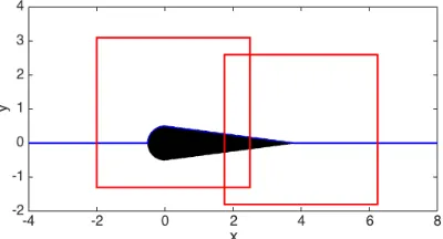
2.2 Time-averaged 2D DNS results for Re= 150 . . . 22
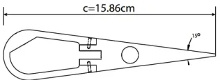
2.3 Schematic of the idealized airfoil . . . 23
2.4 Experimental setup of the flow around an idealized airfoil . . . 24
2.5 Subdivision of the domain into cells . . . 40
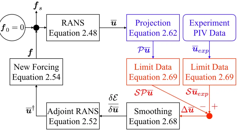
2.6 Block diagram representation of the adjoint looping procedure . . . . 43
3.1 Cartoon of resolvent modes for various amplification mechanisms . . 53
3.2 Pseudospectra and resolvent norm for example operators . . . 58
3.3 Projection of first resolvent mode onto eigenvectors . . . 60
3.4 Spectrum and pseudospectrum of the cylinder base flow at Re=47 . 61 3.5 Stability and resolvent modes for the cylinder base flow at Re= 47 . 63 3.6 The adjoint eigenmode, forward eigenmode, and wavemaker for cylin-der flow at subcritical Reynolds numbers . . . 64
3.7 Spectrum and pseudospectrum of the cylinder mean flow atRe =100 65 3.8 Resolvent norm for subcritical base flows and supercritical mean flows 66 3.9 Wavemakers computed from stability and resolvent modes . . . 68
3.10 Turbulent mean velocity and mean shear profiles for channel flow at Reτ =2000 . . . 69
3.11 |φˆ1(y)|and|ψˆ1(y)|for the near-wall cycle mode where (kx,kz,c+) = (4π,40π,14) . . . 70
3.12 Spectrum and pseudospectrum of the near-wall cycle mode . . . 71
3.13 First 20 singular values of the near-wall cycle mode . . . 71
3.14 |φˆ1(y)|and|ψˆ1(y)|for the near-wall cycle mode where (kx,kz,c+) = (π/9,2π/3,22) . . . 72
3.15 Spectrum and pseudospectrum of the VLSM mode . . . 72
3.17 |φˆ1(y)|and|ψˆ1(y)|for the stationary disturbance mode where (kx,kz,c+) =
(0,2π/3,0) . . . 74
3.18 Spectrum and pseudospectrum of the stationary disturbance mode . . 75
3.19 First 20 singular values of the stationary disturbance mode . . . 75
4.1 First two singular values for mean cylinder wake at Reynolds num-bers where flow is 2D . . . 80
4.2 Schematic defining recirculation lengthlm . . . 80
4.3 Unscaled and scaled mean profiles at recirculation point for 2D cylin-der flow . . . 81
4.4 Unscaled and scaled mean profiles at recirculation point for square cylinder and 3D cylinder flows . . . 82
4.5 Unscaled and scaled base profiles at supercritical Reynolds numbers . 82 4.6 Unscaled and scaled profiles of the first resolvent modes along the centerline . . . 83
4.7 Mean profile on centerline and vortex convection velocity . . . 85
4.8 Recirculation bubble length, shedding frequency, and position of vortex cores . . . 86
4.9 First two singular values forRe =100 mean cylinder wake . . . 87
4.10 ψˆ1and ˆψ2at variousωfor Re= 100 mean cylinder wake . . . 89
4.11 Unscaled and scaled profiles on centerline for resolvent modes at variousωfor Re= 100 mean cylinder wake . . . 90
4.12 Comparison of resolvent and DMD modes for Re =100 cylinder flow 91 4.13 Discrepancy between resolvent and DMD modes forRe =100 cylin-der flow . . . 92
4.14 Nonlinear forcing at 2ωs vs. self-interaction of ˆψ1 . . . 93
4.15 Velocity response modes generated by forcing theH(2ωs) resolvent operator with ˆψ1(ωs)· ∇ψˆ1(ωs) . . . 94
4.16 Discrepancy between the forced resolvent and DMD modes forRe = 100 cylinder flow . . . 94
4.17 Velocity response modes generated by forcing theH(3ωs) resolvent operator with an approximated ˆf(3ωs) . . . 97
4.18 Nonlinear forcing at the shedding frequency . . . 98
4.19 Projection of nonlinear forcing onto resolvent forcing mode . . . 99
4.20 Instability regimes in cylinder flow . . . 100
4.21 Triadic interactions in Re= 100 cylinder flow . . . 102
5.2 Reconstructed pressure and components of mean forcing for
mea-surements on the whole domain . . . 106
5.3 Absolute pressure discrepancy for initial guess, assimilation with-out pressure measurements, and assimilation with surface pressure measurements . . . 107
5.4 Least stable eigenvalue at various stages of the data-assimilation . . . 109
5.5 Pressure correction factor predicted by resolvent modes compared to DNS . . . 110
5.6 Reconstructed mean forcing for various truncated domains . . . 112
5.7 Data-assimilation results for 3D cylinder flow . . . 115
5.8 fxcomparison for 3D cylinder flow . . . 115
5.9 ∇ × f comparison for 3D cylinder flow . . . 116
6.1 Experimental and base flow comparison for idealized airfoil . . . 119
6.2 Full-field mean velocity reconstruction for idealized airfoil . . . 120
6.3 Reconstructed f for idealized airfoil . . . 121
6.4 Reconstructed∇ × f for idealized airfoil . . . 122
6.5 Effect of resolution on mean velocity reconstruction for idealized airfoil123 6.6 Effect of resolution on forcing reconstruction for idealized airfoil . . 124
6.7 Effect of domain on mean velocity reconstruction for idealized airfoil 125 6.8 Effect of domain on forcing reconstruction for idealized airfoil . . . . 126
6.9 Divergence of idealized airfoil velocity fields . . . 127
6.10 Residual discrepancy of idealized airfoil . . . 128
6.11 Mean velocity reconstruction for NACA 0018 airfoil at α = 0◦and Re =10250 . . . 129
6.12 Reconstructed f for the NACA 0018 airfoil atα= 0◦andRe =10250130 6.13 Reconstructed∇ × f for the NACA 0018 airfoil atα= 0◦andRe = 10250 . . . 131
6.14 Mean velocity reconstruction for the NACA 0018 airfoil at α = 0◦ and Re= 20700 . . . 132
6.15 Reconstructed∇ × f for the NACA 0018 airfoil atα= 0◦andRe = 20700 . . . 132
6.16 Mean velocity reconstruction for the NACA 0018 airfoil atα = 10◦ and Re= 10250. . . 133
6.17 Reconstructed ∇ × f for the NACA 0018 airfoil at α = 10◦ and Re =10250 . . . 134
7.2 First three singular values of the NACA 0018 airfoil at α = 0◦and
Re =10250 . . . 140
7.3 Comparison of ˆφ1 forωg = 12.24 of the NACA 0018 airfoil atα = 0◦andRe =10250. . . 141
7.4 DMD eigenvalues of the NACA 0018 airfoil atα=0◦andRe =10250142
7.5 Comparison of ˆψ1 and its DMD counterpart for the globally most amplified frequency of the NACA 0018 airfoil at α = 0◦and Re =
10250. . . 143
7.6 Resolvent and DMD mode comparison at various frequencies for the
NACA 0018 airfoil atα=0◦andRe =10250 . . . 144
7.7 Resolvent modes using an approximated nonlinear forcing at ω =
24.49 . . . 145 7.8 Resolvent modes using an approximated nonlinear forcing atω =2.90146
7.9 Probe points for NACA 0018 at α=0◦andRe =10250 flow
recon-struction . . . 147
7.10 Power spectrum at points P4 and P7 in the airfoil wake . . . 148
7.11 Time traces of the reconstructedv-component when the probe point
is located at P4 . . . 149
7.12 Time traces of the reconstructedv-component when the probe point
is located at P7 . . . 150
7.13 Reconstructed flow att =0 using rank-1 modes for the NACA 0018 airfoil atα =0◦andRe =10250 . . . 151
7.14 Fluctuatingv-component at Point P7 . . . 153
7.15 Reconstructed flow for various times using all modes for the NACA
0018 airfoil atα=0◦andRe =10250 . . . 153
7.16 Reconstructedu-velocity using the flow reconstruction procedure and
various numbers of frequencies . . . 157
7.17 pfor the NACA 0018 airfoil atα=0◦andRe =10250 . . . 158
B.1 First two singular values of the NACA 0018 airfoil at α = 10◦and
Re =10250. . . 182 B.2 Points where the power spectrum is computed for theα= 10◦flow . 183
B.3 PSD of two points in theα=10◦flow . . . 184
B.4 Resolvent response modes computed for the flow around a NACA
0018 airfoil atα=10◦andRe =10250. . . 184
B.5 Resolvent forcing modes computed for the flow around a NACA
LIST OF TABLES
Number Page
2.1 Operator form of the equations for stability and resolvent analyses . . 29
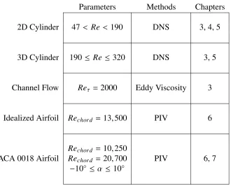
2.2 Summary of flows considered . . . 46
3.1 Quantification of non-normality for cylinder and channel flow . . . . 76
5.1 Cylinder data-assimilation results . . . 104
6.1 Idealized airfoil data-assimilation results. . . 119
7.1 Points used in the NACA0018 airfoil atα =0◦andRe =10250 flow reconstruction . . . 147
7.2 Comparison of the global error for different input points, velocity
NOMENCLATURE
(·)+. pseudo-inverse.
α. angle of attack.
αs. stall angle.
β. step size in new descent direction.
∆u. discrepancy velocity between experiment and simulation.
∆p. discrepancy pressure field between experiment and simulation.
γ. eigenvector of companion matrix.
Λ. diagonal matrix of eigenvalues.
Φ. resolvent forcing modes or right singular vectors of the resolvent operator.
Ψ. resolvent response modes or left singular vectors of the resolvent operator.
Σ. diagonal matrix containing the singular values of the resolvent operator.
υ. DMD eigenvector.
A. LNS operator with respect to the base flow.
A∗. adjoint LNS operator with respect to the base flow.
B. projector to velocity space.
C. restriction operator.
E. a perturbation matrix.
f. mean forcing or the divergence of the Reynolds stress tensor.
f0. nonlinear forcing.
fs. solenoidal component of mean forcing field.
G. stiffness matrix for 1D case.
I. identity matrix.
J. forcing operator.
K. response operator.
L. LNS operator with respect to the mean flow.
L∗. adjoint LNS operator with respect to the mean flow.
M. 2-by-2 model operator.
Q. generic, nonsingular operator.
R. Reynolds stress tensor.
r. vector containing the ratio of singular vector inner products.
S. companion matrix in the DMD algorithm.
T. linear mapping between snapshot matrices.
U. left singular vectors of an arbitrary matrix.
u. velocity field.
u0. fluctuating velocity field.
u†. adjoint velocity field.
U0. base flow velocity field.
V. matrix of eigenvectors.
W. right singular vectors of an arbitrary matrix.
X. snapshot matrix.
X#. displaced snapshot matrix. ˇ
(·). time-resolved measurement.
χ. complex amplitude of a resolvent response mode.
∆t. non-dimensional time step.
η. wall-normal vorticity.
ˆ
(·). resolvent analysis. ˆ
φ. a resolvent forcing mode.
ˆ
ψ. a resolvent response mode.
κ. condition number.
Λ. set of eigenvalues or spectrum of operator.
Λ. pseudo-spectrum of an operator.
λl s. least stable eigenvalue.
h,i. scalar product associated with the energy in the whole domain.
hik. Fourier component associated with wavenumber vector.
D. wall-normal derivative operator.
E. data-assimilation cost function.
H(ω). resolvent operator.
L. full OS-SQ system.
LOS. Orr-Sommerfeld operator.
LSQ. Squire operator.
N. quadratic nonlinearity operator.
P. operating representing the smoothing procedure.
Q. agreement metric between PIV data and the data-assimilation.
R. resolvent of a generic, nonsingular operator.
S. projection operator which artificially truncates PIV data.
W. wavemaker region.
µ. eigenvalue of companion matrix.
Ω. flow domain.
ω. temporal frequency.
ωs. vortex shedding frequency.
u. mean velocity field.
uex p. experimental mean velocity field.
χ. complex weight or expansion coefficient of a resolvent response mode.
p. mean pressure field.
ρ. density.
σ. singular value of the resolvent operator.
τw. wall shear stress.
Θ. spectral radius. ˜
(·). stability analysis.
˜
g. left eigenvector of a generic, nonsingular operator.
˜
g. right eigenvector of a generic, nonsingular operator.
ϕ(x). area averaging operator.
ξ. scalar associated with divergence part of mean forcing field.
ζ. weight associated with a measurement in the data-assimilation algorithm.
a. vortex acceleration.
As. amplitude of shedding mode.
AR. aspect ratio.
C. a complex constant.
c. wavespeed.
D. cylinder diameter.
d. mean shear in model operator.
E. global error of flow reconstructed field.
h. channel half-height.
I(t). instantaneous error for flow reconstruction.
kx. streamwise wavenumber.
kz. spanwise wavenumber.
L. characteristic length scale.
lm. recirculation bubble length.
m. complex eigenvalues of model operator.
N. number of mesh points.
ns. number of stall cells.
p. pressure field.
P0. base flow pressure field.
q. spatial wavelength of resolvent mode.
Re. Reynolds number.
Rechor d. chord-based Reynolds number.
Recrit. critical Reynolds number.
U. characteristic velocity scale.
Uc. vortex convection velocity.
U∞. free-stream velocity.
uτ. friction velocity.
z. generic complex number.
LES. Large-eddy simulation.
LNS. linear Navier-Stokes.
OS. Orr-Sommerfeld.
C h a p t e r 1
INTRODUCTION
1.1 Motivation
Practical implementation of closed-loop control of complex fluid systems has so far
remained elusive due to a number of challenges. These include a lack of under-standing of the dominant physics, the nonlinearity of the governing equations, and
the wide range of scales inherent to the problem. Despite these obstacles, several
studies such as Bewley et al. (2001) have successfully relaminarized wall-bounded
turbulent flows using adjoint-based optimal control theory. The control algorithm
in Bewley et al. (2001) had access to full state information or knowledge of all flow
quantities at every grid point. This is not feasible experimentally so an estimator
is necessary to deduce states which are not directly measured. Figure 1.1(a) is a
schematic of a typical closed-loop flow control configuration where the estimator
measures the flow and the controller actuates on it. The design of an effective es-timator, however, is not straightforward as the questions of where to measure in
the flow and which flow states should be measured have no clear answers. They
are frequently flow dependent and may be sensitive to small changes in the flow
configuration.
This thesis focuses on obtaining the maximum amount of information from the
flow from the fewest measurements possible. To meet this challenge,
fundamen-tal questions about reduced-order modeling and data-assimilation are addressed. Reduced-order models capture the essential features of a flow and the advantage of
such an approach is to gain insight of the flow physics in order to identify
mecha-nisms for controlling the flow (Rowley and Dawson, 2017). If a suitable basis for
the flow can be determined, then it can be reconstructed with reasonable fidelity
using a small subset of basis functions. Another approach to flow reconstruction
is data-assimilation whereby experimental measurements are merged with
compu-tational fluid dynamics (CFD) to improve prediction of real-world flows (Hayase,
2015) as seen in Figure 1.1(b). The underlying principle is to complement CFD,
which lack full fidelity, with limited experimental measurements so that the
(a) (b)
Figure 1.1: Comparison of the elements in a closed loop control arrangement (a) with data-assimilation (b).
1.2 A Musical Analogy
Before introducing background literature on the technical aspects of this thesis, the
author would like to offer a musical analogy for reduced-order modeling and flow
reconstruction. No musical knowledge is necessary to understand this analogy. In
addition to being able to visualize music by looking at the notes written on a page
or watching a pianist’s hands move, for example, music can be heard. In fact, it
is easier to judge whether the notes written on a page sound ‘right’ by hearing them being played. Thus, music has an edge over fluid mechanics when deciding
whether or not a reduced-order model captures the essential components of a piece
or song. One might ask when reduced-order modeling is necessary in the first
place since there are no pieces written by composers which cannot be performed as
long as there are enough musicians to cover the parts and they have the technical
skills necessary to play it well. It turns out that reduced-order modeling is used all
the time and the particular example that will be discussed below is arranging the
orchestra accompaniment to a concerto for piano.
1.2.1 Concertos and Arranging
A concerto is a musical composition written for a solo instrument with the orches-tra accompanying. The solo part tends to be virtuosic and technically demanding
in order to showcase the soloist’s mastery of the instrument. It also contains the
principal themes and melodies of the piece. The orchestra, which is made up of
many instruments, plays a supporting role by providing harmonies and background
atmosphere. Concertos can be written for any instrument although the piano is the
most common followed by the violin. Since the orchestra consists of as many as
eighty people, it is not practical for a soloist auditioning on a piece to have full
orchestra accompaniment. This would involve coordinating the schedule of many
practicing their parts and turning up to rehearsal! Instead, it is far more practical
for the orchestra part to be arranged for piano and for the soloist to audition with a
piano accompanist. As one might guess, the pianist cannot play the orchestra part to full fidelity so a reduced-order model is necessary to arrange the music such that
it is playable by a single pianist.
Accomplishing such a task is not straightforward and requires pretty advanced
knowledge of not only music theory but also the piano. To begin with, the
pi-anist has only two hands which have a limited amount of reach. While it is possible
to play many notes at once, the hand can maybe reach between an interval of nine
keys on the piano. There are physical limitations, therefore, that the arranger needs
to consider. The musical constraints are less obvious and are harder to satisfy by a brute force approach. For instance, if the arranger were to simply take all the
orchestra parts and write them on the same page at once, it would immediately
be-come obvious that some instruments are playing the same notes at the same time.
Thus a part is being doubled and so the arranger has already accounted for two
in-struments. Occasionally the same notes at different frequencies are being played
simultaneously — think of men and women singing Happy Birthday at an office
party. They are singing the ‘same’ notes but at different pitches since men tend to
have deeper voices than women. In physics, one would think of a fundamental
fre-quency f1 and higher harmonics 2f1, etc. In music, these are called octaves since
2f1would be the eighth note after f1in a musical scale.
1.2.2 Structure and Statistics
Instead of turning to physics and governing equations such as Navier-Stokes, the
arranger makes use of music theory. Figure 1.2 is the beginning of Schubert’s
Impromptu No. 3 Opus 90 in G-flat major. This piece is for solo piano and one
reads the music from left to right like a book. The pianist reads two lines together:
the right-hand plays the upper staff, which is a collection of five horizontal lines,
while the left-hand plays the bottom staff. The two staffs are connected by vertical
lines denoting measures, or musical subunits, and the notes appear on individual
lines or spaces with respect to the staff. A high placement of a note on the staff denotes a high pitch and vice versa for low notes.
Three different colored boxes appear in Figure 1.2 to denote the three ‘structures’
which appear in the music. The part or voice in the solid red box is the melody
Figure 1.2: The first two lines of Schubert’s Impromptu No. 3 in G-flat Major Opus 90. The melody is contained in the red solid box, the bass line in the dashed blue box, and the ornamentation in the brown dotted box. The thickness of the boxes indicates the relative volume at which each of these lines should be played.
is the most important voice and should be played the loudest which is why the red box has the thickest lines. The bass is the voice contained in the dashed blue box
and is played by the left hand. It is the second most important voice by supporting
the melody and enriching the overall sound of the music. Last, and certainly least
in terms of importance, is the ornamentation in the dotted brown box which has the
thinnest lines. The purpose of the third voice is to add atmosphere and movement
creating a shimmering effect. Incidentally, this voice is what makes the piece
chal-lenging since the ornamentation is played by the strong fingers (thumb, pointer, and
middle) of the right hand while the melody is in the weaker fingers (ring and pinky).
The structure in complex flows is also quite important, as they typically account
for a large amount of the fluctuating energy. While the structures in Figure 1.2 are
relatively easy to identify given their spatial separation on the staff, identifying them
in flows tends to be more challenging, warranting the use of modal decomposition
techniques which are introduced in Section 1.3. Some of these make use of the
statistics of the flow such as the time-averaged velocity field. The ‘statistics’ in
music are the key and time signatures which are located at the very beginning of
the piece. The key signature is made up of]and[ symbols, of which there are six
of the latter in Figure 1.2, and denotes the key or scale the piece is based on. There are chords (combinations of notes) which are particular to each key and these often
play an accompanying role in music. The time signature in Figure 1.2 is indicated
in a measure. Implicitly, this suggests what types of rhythms are likely to appear as
well as which beats should be emphasized more than others.
In short, the voices in music can be likened to coherent structures in flows which
have varying degrees of importance. The time and key signatures are similar to
statistics which, using music theory or the governing equations, may yield useful
information about the actual piece or flow.
1.2.3 Beethoven Violin Concerto
The arranger considers both the structure and statistics of the piece when
attempt-ing to build a reduced-order model of the orchestration. Two fragments of the
Beethoven Violin Concerto are reproduced below to observe how the arranger took
music which was originally written for full orchestra and simplified it for piano. In
Figure 1.3, the parts for each instrument appear all together and the piano arrange-ment appears as the last two lines. The arranger has, in fact, written the original
instruments next to the parts the piano is playing. In Figure 1.3, the piano is able
to play almost all the notes played by the orchestra. Even though the reduced-order
model (piano arrangement) very faithfully reconstructs the original orchestration,
it loses the distinct sound, or timbre, of each instrument such as the oboe vs. the
clarinet. It is impossible, therefore, for the piano to capture everything.
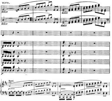
Another fragment of the piece is reproduced in Figure 1.4 where the piano
arrange-ment is the final two lines and the orchestration is the top seven lines. Here, the arranger needs to make some choices since the pianist cannot play all the notes
from the original orchestration. The first notes of lines 1 and 2, for example, are the
same notes at different frequencies or octaves. The arranger has decided, therefore,
to choose just line 1 which is played by the right-hand. The arranger has also
sim-plified Lines 4-7 since the pianist’s left-hand cannot play all four notes together at
the speed written. To make the music playable, Line 4 is omitted since it is covered
by the right-hand and the left-hand alternates between Lines 6/7 and Line 5. All
the notes from the orchestration are being played, just at a slightly lower temporal
frequency. This type of trick makes it much easier for the pianist since the playing of repeated sixteenth notes can be avoided.
There are many videos online which visualize arrangements of music for solo piano
while they are being played. Thus one can hear and see a reduced-order model
although a true assessment of its fidelity is to study the music. The rest of the thesis
Figure 1.4: A second excerpt of Beethoven’s violin concerto where the top seven lines are the orchestration and the bottom two are the piano arrangement.
principles. Perhaps one advantage fluid mechanics has over music is that success or
optimality can be measured mathematically. It will be seen, however, that the way
optimal is defined might not yield the best answer so it might be necessary to make
use of other tricks akin to the one used by the arranger to avoid repeated sixteenth
notes.
1.3 Reduced-Order Modeling
There are numerous modal decomposition techniques which have been applied to
analyze flows. In the overview of Taira et al. (2017), techniques which use flow data
as an input are classified asdata-basedwhile techniques which rely on a more
the-oretical framework or discrete operators from the Navier-Stokes Equations (NSE)
for flow reconstruction if only a small number of time-resolved measurements are
available. It becomes important, consequently, to understand the conditions under
which an operator-based technique identifies meaningful structures which actually appear in the flow. This section reviews recent progress and challenges with
re-spect to coherent structure eduction with an emphasis on resolvent analysis using
the time-averaged mean as an input.
1.3.1 Stability of the Mean Flow
A time-averaged flow, or mean, that is statistically stationary can often be defined
and leveraged using the eigenvalue spectrum of the governing NSE to educe the
frequencies, i.e. the imaginary part of the eigenvalues, and shapes of coherent
structures which appear in the flow. Recent studies have demonstrated the
suc-cess of mean flow stability analysis for a variety of flows including thermosolutal
convection (Turton et al., 2015), turbulent jets (Gudmundsson and Colonius, 2011;
Oberleithner et al., 2014; Schmidt et al., 2017a), and flow over a backward facing step (Beneddine et al., 2016). There is also a significant body of work discussing
stability analysis of the mean cylinder wake which was shown by Barkley (2006)
to correctly identify the frequency of the globally unstable flow above the
criti-cal Reynolds number of Re = 47 (Provansal et al., 1987; Sreenivasan et al., 1987;
Noack and Eckelmann, 1994). Notably, classical linear stability analysis of the base
flow, which is an equilibrium solution of the NSE, at supercritical Reynolds
num-bers does not predict the correct observed frequency. The base (laminar) and mean
(time-average of the fluctuating velocity field) profiles are differentiated because of
the importance of nonlinearity in sustaining the latter.
The two-dimensional von-Kármán vortex street becomes unstable to three-dimensional
perturbations at a Reynolds number of Re = 189 (Barkley and Henderson, 1996;
Williamson, 1996). A global stability analysis of the span-averaged mean wake
continues to identify the shedding frequency as demonstrated by Leontini et al.
(2010). Recent work has endeavored to explain why and when mean stability
anal-ysis is valid. Barkley (2006) suggested that success corresponds to cases where the
Reynolds stresses are unperturbed at order when considering infinitesimal per-turbationsu˜(x,y)exp(λt) to the mean flow solution. This was confirmed by Sipp
and Lebedev (2007) who determined that the nonlinear interaction of the leading
global mode with its conjugate, i.e. the contribution to the mean Reynolds stresses,
significantly outweighed the interaction of the mode with itself leading to higher
can be approximated with the leading global mode and its conjugate.
1.3.2 Resolvent Analysis
Sipp and Lebedev (2007) used open cavity flow as a counter example to the validity
of mean stability analysis where the predicted frequencies do not match direct
nu-merical simulation (DNS) of the flow. This discrepancy can be attributed to the non-normality of the flow which leads to non-orthogonality of the global modes and
sen-sitivity of the spectrum to perturbation of the operator (Trefethen et al., 1993). The
behavior of these systems can be more accurately characterized by the
pseudospec-trum of the LNS operator using resolvent analysis, e.g., Trefethen et al. (1993)
and Schmid and Henningson (2001), rather than the spectrum alone. Jovanovi´c
and Bamieh (2005) formulated the linearized problem for laminar channel flow in
input-output terms, where the resolvent operator constitutes the transfer function
between them, considering the component-wise transfer from harmonic exogenous
disturbance or forcing (input) to velocity response (output). There is also a broad literature considering stochastic forcing, e.g., Farrell and Ioannou, 1993, and the
initial condition, transient growth problem, e.g., Butler and Farrell, 1992.
McKeon and Sharma (2010) and Hwang and Cossu (2010) considered the resolvent
reformulated with respect to the turbulent mean flow for canonical turbulent wall
flows. The latter authors employed an eddy viscosity to account for the action of
the Reynolds stresses, while the former analysis extends the approach to include
the nonlinear terms as the input forcing to the linear operator, i.e. closing the feed-back loop. McKeon and Sharma (2010) performed a singular value decomposition
of the resolvent to identify the inputs giving rise to the most amplified responses
which are ranked by their gain (singular value). The approach has been extended
to non-parallel flows, e.g., Lu and Papadakis (2014), Beneddine et al. (2016), Jeun
et al. (2016), and Schmidt et al. (2017b). Beneddine et al. (2016) concluded that
mean stability analysis was valid when the dominant singular value of the resolvent
operator was significantly greater than the others at a given frequency and that this
condition holds for flows where there is a dominant convective instability
mecha-nism and an eigenvalue which is nearly marginally stable. In such circumstances, it was shown that the eigenmodes are proportional to the resolvent response modes.
Stability and resolvent analyses are formally related in Chapter 3 by a dyad
1.3.3 Non-normality
Subsequent to the work of Jovanovi´c and Bamieh (2005), Marquet et al. (2009) and
Brandt et al. (2011) investigated the distribution of energy and phase between the
velocity components of the most amplified input/output in analyses about laminar,
base flows in recirculation bubbles and the flat plate boundary layer, respectively.
These studies distinguished between component-type non-normalities, which
dis-tribute energy in different velocity components, and convective non-normalities,
which separate the spatial support of forcing upstream of the response. The roots of these non-normalities are the mean shear and mean flow advection terms,
re-spectively, in the linearized NSE. These terms also result in the Orr mechanism
(Orr, 1907), which reorients upstream-leaning forcing modes with the mean shear
such that the response modes are leaning downstream (Farrell, 1987). Chomaz
(2005) quantified non-normality via the inner product between the most amplified
input and output. A response dominated by non-normality results in a smaller inner
product and this has an impact on the amplification mechanisms identified by the
resolvent.
1.3.4 Instabilities and Pseudoresonance
The response of a system to harmonic input (forcing) can be classified as resonant or pseudoresonant. The latter occurs due to nonmodal effects associated with the
sensitivity of the spectrum to perturbation (Trefethen et al., 1993). The former is
generally an instability mechanism and corresponds to excitation in the vicinity of
an eigenvalue. Instability mechanisms can be further classified as convective or
ab-solute depending on the nature of the base or mean flow. A convective instability is
one where perturbations grow downstream as they are swept away by the flow while
an absolute instability is one where perturbations grow upstream and downstream
of where they originated (Huerre and Monkewitz, 1985; Schmid and Henningson,
2001). The presence of reverse flow tends to result in a region of absolute instabil-ity (Rowley et al., 2002; Suponitsky et al., 2005; Juniper, 2012). The nature of the
instability, thus, has a bearing on the strength of the component-type non-normality
mentioned earlier and this is explored in Chapter 3.
1.3.5 Data-Driven Methods
Resolvent analysis also has relationships with data-driven methods such as
Dy-namic Mode Decomposition (DMD). Introduced by Schmid (2010), DMD extracts
demonstrated the similarity between resolvent modes and DMD modes
correspond-ing to the same temporal frequency in turbulent pipe flow. DMD is also related to
the Koopman operator (Rowley et al., 2009), or an infinite-dimensional linear op-erator associated with the full nonlinear system. This is significant since Sharma
et al. (2016a) later noted that both DMD and resolvent modes may approximate the
‘true’ Koopman modes of the system.
Other connections between resolvent analysis and data-driven methods, in
particu-lar spectral proper orthogonal decomposition (SPOD), have been expounded upon
by Towne et al. (2018). Originally introduced by Lumley (1970), SPOD results in
modes which are orthogonal in space and time. They can be interpreted, therefore,
as optimally averaged DMD modes which are obtained from an ensemble DMD problem. Connections were also drawn between SPOD and resolvent analysis.
When the input forcing to the resolvent operator can be approximated as
white-noise, resolvent modes are identical to SPOD modes. It has been noted by, e.g.,
Zare et al. (2017) that white-in-time stochastic forcing is insufficient to explain
tur-bulent flow statistics and, in instances where the forcing is correlated, differences
arise between the SPOD and resolvent modes. Schmidt et al. (2017b) demonstrated
this phenomenon for low temporal frequency modes in a turbulent jet.
While SPOD is not considered here, its connection to DMD and resolvent analysis
is useful as it suggests there are cases when the modes predicted by resolvent
anal-ysis will not match DMD modes computed directly from the data. The conditions
under which these circumstances are likely to arise will be addressed. Since this has
an impact on flow reconstruction as noted by Towne et al. (2018), the nature of the
nonlinear forcing needs examination to correctly identify the structures in the flow
when the forcing cannot be treated as white-noise (McKeon et al., 2013; McKeon,
2017).
1.4 Data-Assimilation
It has been noted in several studies (Nisugi et al., 2004; Suzuki et al., 2009a; Suzuki
et al., 2009b; Suzuki, 2012; Foures et al., 2014) that despite recent advances in computational fluid dynamics (CFD) and experiments, both techniques have several
disadvantages. Despite capturing the "true" physics of the flow, for example,
exper-iments are corrupted by noise, limited by field of view, and have insufficient
reso-lution to capture small scales. CFD, on the other hand, requires modeling
computational power to resolve all scales in turbulence. Data-assimilation (Lewis
et al., 2006) is a technique whereby experimental measurements can be merged
with computational fluid dynamics (CFD) to improve prediction of real-world flows (Hayase, 2015). The underlying principle is to complement CFD, which lack full
fidelity, with experimental measurements, which typically lack full-field
informa-tion, so that the simulation reflects the dynamics observed in the laboratory. The
assimilated or hybrid flow is able to recover quantities in the experiment which
would otherwise be inaccessible or difficult to measure such as pressure, vorticity,
and Reynolds stresses, by reducing noise and improving resolution. It is also
possi-ble to extrapolate the flow beyond the experimental view by solving the equations
on a larger domain.
Data-assimilation can be traced back to meteorology (Le Dimet and Talagrand,
1986) and is of particular interest to the experimental fluid mechanics community
since it may be used to complete experimental observations by enforcing
dynam-ical constraints (Heitz et al., 2010). One of the first hybrid simulations conducted
by Nisugi et al. (2004) used offline, sequential assimilation for flow behind a square
cylinder. By measuring the discrepancy between experimental and numerical
pres-sure meapres-surements at finite time intervals to drive the momentum equations, the
simulation was altered to match the experiment. Sequential assimilation was greatly
expanded by Suzuki et al. (2009a) and Suzuki et al. (2009b) when particle-tracking velocimetry (PTV) data of an airfoil at high angle of attack was fed into a
two-dimensional direct numerical simulation (DNS). The resulting hybrid flows
con-tained less noise and recovered the unsteady pressure fields. They also offered
insight into the statistics of the mean flow and the three-dimensional instabilities
which attenuate vorticity strength.
1.4.1 Variational Methods
Data-assimilation has also been extended to the NSE using a variational approach
(Papadakis and Mémin, 2008; Gronskis et al., 2013; Foures et al., 2014) where,
similar to optimal control, the objective is to minimize a cost function. This
gener-ally involves penalizing the distance between experimental and numerical velocity fields subject to governing equations. Ensemble Kalman filter or ensemble-based
variational approaches (Colburn et al., 2011; Suzuki, 2012; Kato et al., 2015; Silva
and Colonius, 2017) rely on the Kalman filter and its ensemble variant (Kalman,
1960; Evensen, 1994), which are appropriate when the data-assimilation problem
can be traced back to optimal control theory, which has been applied to various
flow control problems (see Kim and Bewley, 2007, for an overview). Bewley et
al. (2001) studied the control side of the problem by investigating various con-trol strategies applied to turbulent channel flow simulated using a DNS.
Data-assimilation, on the other hand, functions more closely to an estimator which reads
in inputs from various sensors and fits them to an underlying model. The idea is to
read in a sparse number of measurements and use the model to produce an estimated
state which is more highly resolved in space and time.
Foures et al. (2014) used a variational method to minimize the discrepancy between
the mean velocity fields of a DNS and an incompressible RANS simulation for flow
around a circular cylinder at a Reynolds number ofRe =150.An improved estima-tion technique for mean flows has potential applicaestima-tions in mean flow modificaestima-tion
studies. A large body of work has attempted to investigate this problem which has
its roots in the experiments of Strykowski and Sreenivasan (1990), who showed
ex-perimentally that for low Reynolds numbers, a small control cylinder inserted in the
wake behind a larger cylinder can completely suppress vortex shedding. Numerical
studies including Giannetti and Luchini (2007) and Marquet et al. (2008) looked
at the sensitivity of the cylinder instability to base flow modification and steady
forcing near critical Reynolds numberRecrit. Meliga et al. (2012) and Mettot et al.
(2014) expanded this framework to higher Reynolds numbers and determined how a small control cylinder could impact the frequency of vortex shedding as predicted
by the most unstable global mode of the mean flow. Data-assimilation could
ex-pand control techniques to wall actuators such as an oscillating ribbon or synthetic
jet which are difficult to model computationally due to ambiguous boundary
con-ditions at the wall. It is possible, for example, to determine the mean flow from an
experiment and recover a more highly resolved mean flow by tuning the boundary
condition at the wall so that the simulated mean flow matches the experimental one.
A study conducted by Gronskis et al. (2013) illustrates this point quite well. They
employed adjoint data-assimilation to generate initial and inflow conditions for a
DNS of flow around a cylinder at a Reynolds number of Re = 172. The
result-ing simulation reflected the flow physics from large scale PIV measurements but
contained far lower noise levels. Data-assimilation has also been demonstrated
by Mons et al. (2016) to be applicable for perturbed fluid problems. They
com-pared variational, ensemble Kalman filter-based, and ensemble-based variational
co-herent gusts. They found that the variational data-assimilation approach produced
the best results since the adjoint method can effectively capture the first-order
sensi-tivity of the cost functional which penalizes the distance between experimental and numerical velocity fields.
1.4.2 Incorporating Pressure and Extension to Experiments
In this thesis, the algorithm of Foures et al. (2014) is modified to include mean
pres-sure meapres-surements since, without prespres-sure data, only the solenoidal component of
the forcing to the mean momentum equations can be recovered. The irrotational
component is lumped into the mean pressure gradient term, which prevents
recov-ery of the mean pressure field. It is possible to solve a Poisson equation for mean
pressure using the RANS equations, e.g., Oudheusden (2013), but this relies on
computing two gradients of the Reynolds stresses which suffer from noise
contam-ination. One can ask whether limited mean pressure measurements can account
for this problem and where in the flow do they have the greatest impact. Recent studies, e.g., Kang and Xu (2012), Mons et al. (2017), and Manohar et al. (2017),
have investigated optimal placement of sensors for flow reconstruction and this is
addressed in the thesis. The framework of Foures et al. (2014) is also adapted
to mean flows obtained from experimental data at significantly higher Reynolds
numbers. The mean profiles are obtained from time-averaged particle image
ve-locimetry (PIV) data from a free-surface water tunnel. The necessary experimental
parameters such as field of view or vector resolution for successful mean flow
re-construction are addressed.
1.5 Flow Reconstruction
A growing number of studies have investigated flow reconstruction using resolvent modes as a basis. Analysis of the linear operator via the singular value
decompo-sition only does not yield the complex weights, or expansion coefficients, of the
modes. This has to be calculated by projecting the resolvent forcing modes onto the
nonlinear forcing. One approach adopted by Moarref et al. (2014) was to formulate
a convex optimization problem which optimally reproduced the energy spectra of
a turbulent channel flow. The study led to close agreement with the DNS spectra
using only 12 modes per wall-parallel wavenumber pair and temporal frequency
although the method tended to overpredict the streamwise energy and underpredict
solved for the expansion coefficients by projecting the Fourier-transformed
nonlin-ear term onto the resolvent forcing modes. With 24 modes, a substantial amount of
the acoustic energy predicted by a large-eddy simulation (LES) could be recovered.
Resolvent modes have also been used to find a low-dimensional representation of
exact coherent states of the NSE by Sharma et al. (2016b) and Rosenberg and
McK-eon (2018). In the latter study, the wall-normal velocity and vorticity fields could be
decomposed into their Orr-Sommerfeld (OS) and Squire (SQ) contributions. This
reduced the number of singular modes per wavenumber pair needed to represent
the velocity fields. A Helmholtz decomposition of the nonlinear term, furthermore,
highlighted the role of the solenoidal forcing which could be isolated to determine
its contribution to the OS and SQ modes. It was then possible to obtain an efficient
representation of the wall-normal velocity which was not possible using previous techniques.
A different approach outlined in Towne et al. (2015) and Towne (2016) is to educe
the nonlinear forcing experienced by wavepackets in a Mach 0.9 turbulent jet
us-ing empirical resolvent-mode decomposition. The objective was to identify and
characterize the missing dynamics which were responsible for the failure of linear
wavepacket models to predict acoustic radiation.
Other methods have bypassed consideration of the nonlinear term by taking
ad-vantage of a flow’s low-rank behavior. In such circumstances, the resolvent modes provide an efficient basis for the fluctuations in the flow. Gómez et al. (2016a) and
Beneddine et al. (2016), for example, used resolvent analysis of a lid-driven
cav-ity and backward facing step, respectively, to determine the shapes of the veloccav-ity
fluctuations at various temporal frequencies. Since the dominant singular value of
the resolvent operator was sufficiently greater than all the others, the first resolvent
mode could account for most of the fluctuation energy. It should be emphasized
that this method works if the basis is good and the resolvent operator is low-rank.
There are several examples in this thesis where this is not the case.
A single pointwise unsteady measurement was necessary to calibrate the complex
amplitudes of the resolvent modes. This concept has also been applied by Gómez et
al. (2016b) to estimate forces on a square cylinder, Beneddine et al., 2017 to
exper-imental data of a jet, and Thomareis (2017) to DNS data of airfoils. Each of these
studies noted that the robustness of the reconstruction depended on the location of
the unsteady measurement. They concluded that the unsteady measurement should
improved by using multiple measurements.
1.6 Approach and Outline of Thesis
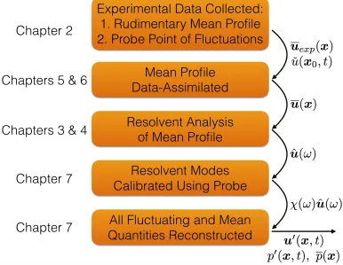
Figure 1.5 is a schematic which outlines the thesis and the procedure for
recon-structing statistically stationary flows with as few measurements as possible. The
first step is to collect experimental data consisting of a rudimentary, in terms of spatial resolution and field of view, mean profile and a single probe point which
contains time-resolved information. Chapter 2 describes the experimental methods
used to obtain the data and provides the mathematical background for the various
modal decomposition techniques used as well as the data-assimilation framework.
Chapter 3 is an original perspective on stability and resolvent analyses for base
and mean flows with an emphasis on the latter. The analyses are formally related
through a dyad expansion and the real part of an eigenvalue, which is difficult to
interpret when the NSE are linearized around the mean flow, is shown to be
im-portant as it influences the degree to which a disturbance is amplified. It also has a bearing on whether or not the resolvent operator is low-rank since an eigenvalue
must be sufficiently separated from the rest of the spectrum in order to dominate
over the contribution of other eigenvalues in the dyad expansion. Non-normality
plays a role in amplification and is investigated through the lens of the
pseudospec-trum (e.g. Trefethen et al., 1993; Reddy et al., 1993; Trefethen et al., 1999; Schmid
and Henningson, 2001; Schmid, 2007; Schmid and Brandt, 2014) of the LNS
oper-ator.
When an eigenvalue is marginally stable, or very close to the imaginary axis, it
drowns out the effect of other eigenvalues over a large range of temporal
frequen-cies. It is shown in Chapter 4 that the most amplified structure for a cylinder at
a Reynolds number of Re = 100 over this range of frequencies is a stretched or
compressed version of the shedding mode. The dominance of this mode leaves
a significant footprint on the mean profile whose geometry scales with the
shed-ding frequency for Reynolds numbers 60 < Re < 320. Similar to Dergham et al.
(2013) for a backward facing step, various branches of singular values are identified
for the cylinder including one for the shedding mode and another for free-stream modes which are less amplified near the shedding frequency. At temporal
harmon-ics, however, the resolvent predicts a structure which is completely different from
its DMD counterpart, suggesting that the structure of the nonlinear forcing has a