Evaluation of baffles for optimisation of waste stabilisation ponds : a thesis presented in partial fulfilment of the requirements for the degree of Master of Engineering in Environmental Engineering at Massey University, Palmerston North, New Zealand

Stabilisation Pond Hydraulics

A thesis presented in partial fulfilment of the requirements For the degree of

Masters of Engineering in

Environmental Engineering

at Massey University, Palmerston North, New Zealand

Jill Helen Harrison

Waste stabilisation ponds are a common form of treating wastewater throughout the world and they provide a reliable, low-cost, low-maintenance treatment system. A literature review undertaken highlighted the need for improved understanding of the hydraulics of such systems, and their upgrade. In particular, the application of baffles is not well understood beyond the use of longer, traditional baffles to increase the approximation to plug flow. The mechanisms and interactions behind baffles are not generally understood.

The work involved the use of CFO modelling to assess various pond designs. In addition to this, traditional tracer studies were carried out on a physical laboratory model, and on a full-scale field pond. These traditional studies highlighted the success of the computer mode II ing approach.

CFO modelling was used to model twenty pond designs, utilising various baffle lengths, number and position. These cases also studied inlet type and outlet position. In the second phase of the work, six of the CFO designs were tested in the laboratory setting. The final phase of work involved two tracer studies carried out on a field pond, utilising a modified inlet, then a combination of a modified inlet and the inclusion of a short (stub) baffle.

CFO modelling has shown to be an effective investigative and design tool. The addition of results from laboratory and field studies further emphasises the benefits of the CFD modelling. The work has also provided an understanding of key flow mechanisms and interactions that have previously been attributed to other factors.

Single baffles are not generally effective, and a mmtmum of two batlles will generally be required to achieve significant treatment improvements. The potential of short (stub) baffies has been shown, however they are sensitive to design changes and should be further researched.

ACKNOWLEDGEMENTS

The completion of a Masterate thesis, while a major individual effort, could not be completed without considerable help and guidance from many people.

Firstly my supervisor, Andy Shilton - for the opportunity and the assistance throughout my period of study. It has been a great opportunity to be part of some ground-breaking research and ideas.

The larger project that this thesis contributes to had considerable funding from the following: the Sustainable Management Fund of the Ministry for the Environment, various City, District and Regional Councils Their assistance is greatly appreciated.

The staff of the Institute of Technology and Engineering, Massey University, deserves mention, all of the Ag Eng Building staff, in particular, Don, Russell and Marcel from the workshop for all the bits and pieces they have fabricated. Richard, Paul and Katie for being a sounding board when it came to write-up time. Roanna for her invaluable help in setting up various documents.

Mention must be made of the help from Claire Driver, a 4th year research student, for her assistance in completing the laboratory modelling program.

There are many people who have helped directly or indirectly, and are too many mention. Thanks go to IPENZ, for the awarding of the Craven Scholarship for Post-graduate Research in Engineering - valuable in easing the financial burden of post-graduate study.

CONTENTS

ABSTRACT ... 1

ACKNOWLEDGEMENTS ... 2

CONTENTS ... 3

TABLE OF FIGURES ... 10

TABLE OF TABLES ... 16

1. INTRODlJCTION ... 17

1.1 1.2 THE NEED FOR THE RESEARCH ... 17

0B.fl--,:C'rIVES AND APPROACH ... ] 8

2. LITERATURE REVIEW ... 19

2.1 2.2 WASTE STAHIIIS/\T!ON PONDS. TYPES OF PONDS ... . .. ... 19

.... 21

2. 2.1. Anaerobic ... 21

2.2.2. f<ctcultative ··· 22

2. 2. 3. Maturation Pond-; ... 2 3 2.2.-1. High-Rate Algal Pond, ... 2-1 2.3 POND DESIGN... ... . ... 24

2. 3. J. 1-oading ]~ates ... 2-1 2. 3. 2. Fmpirical /Jesign f~'quations ... 25

2.3.3. Rational Models ... 25

2.3.3.1. 2.3.3.2. 2.3.3.3. Ideal Flow ... 26

Non-Ideal Flow ... 27

Combined Pond Models ... 28

2. 3.4. Mechanistic Modelling ... 29

2.4 IMPORTANCE OF POND HYDRAULICS ... 31

2.5 FACTORS AFFECTING POND HYDRAULICS ... 33

2.5. J. JnletsDutlet Configuration ... 33

2.5.2. Wind ... 37

2.6 BAFFLES··· 39

2. 6.1. Hydraulic Investigations of Baffle Implementation ... ..JO 2.6.2. Bc([/les & Wind ... ..J6 2. 6. 3. Baffles & Attached Growth Systems ... ..J 7 2.6...J. Nutrient Removal in Baffled WSP ... ..J7 2. 6. 5. Baff! es in Tanks

&

2. 6.8. Bqffles Sun1n1ary ... 51

2. 7 TECHNIQUES FOR ASSESSING POND HYDRAULICS ... 52

2. 7.1. Tracer Studies ... 52

2. 7.2. C'l•'JJ Modelling ... 5-1 2.7.2. l. CFO Modelling by Wood (1997) . . ... 55

2.7.2.2. 2.7.2.3. 2.7.2.4. CFO Modelling by Salter ( 1999) .... . . ... 56

CFO Modelling by Shilton (200 ! ) .. .. .. ... 56

Other Work on CFO Modelling of WSP's ... .. . ... 57

2. 7.3. rahoratory Modelling ... 57

2. 7 . ..J. I )rogue 5,tudies ... 58

2.8 SUMMARY AND CONCUJSIONS ... ... 60

3. l\lETHODOLOGY ... 62

3. I EXPERIMENTAL OVERVIEW. .... 62

3.2 CFO MODELLING.. ... . .... 62

3. 2.1. Introduction to PH()J,;NJCS ... 62

3. 2. 2. Development of the Computer Model ... 63

3.2.3. Simulations lfndertaken ... 6-1 3.2.3.1. 3.2.3.2. Obtaining a Solution ... 64

Non-Steady State Runs ... 66

3. 2. 4. Integrating Reaction Kinetics ... 67

3. 2. 5. Grid Refinement ... 68

3. 2. 6. 71,rbulence ... 71

3.3 CONFIGURATIONS TESTED USING CFD ... 71

3.4.1.1. Reynolds Number versus Froude Number Design ... 74

3...1.2. Froude Number Based Design ... 7-1 3.-1.3. Laboratory Pond Set-up ... 75

3.-1.-1. Tracer Studies ... 76

3.-1.5. Configurations tested in the Laboratory ... 77

3. 5 FIELD STUDIES ... 78

4. RESULTS OF CFO MODELLING ... 82

4.1 OVERVIEW OF CFO MODELS INVESTIGATED ... 82

-I. 1.1. Presentation of Results ... 8-1 4.2 BASIC POND... . ... 85

-I. 2.1. (,ase 1 ... 85

4.2.1.1. 4.2.1.2. Design Rationale Results and Discussion .... ··· ... 85

··· ... 85

4.3 EVENLY SPACED MULTIPLE BAFFLES, STANDARD LENGTH . ... 87

./. 3.1. Case 2 fraditiona! two bciffle design ... 87

4.3.1 I. 4.3.1.2. ./. 3. 2. Case 3 4.3.2.1. 4.3.2.2. ./. 3. 3. Case ./ 43.3.1. 4.3.3.2. Design Rationale ... .87

Results and Discussion.. 87

fraditional four baffle case ... 89

Design Rationale. . ... 89

Results and Discussion.. . ... 89

Traditional six bciffle design ... 91

Design Rationale ... . Results and Discussion ... . 91 92 -1.3../. Case 5 Traditional eight baffle case ... 93

4.3.4.1. Design Rationale ... 93

4.3.4.2. Results and Discussion ... 93

4. 3.5. Sumn1ary ... 95

4.4 UNEVENLY SPACED BAFFLES, STANDARD LENGTH ... 95

4.4. 1. Case 6 Two bcifjles, unevenly spaced. ... 95

4.4.1.1. Design Rationale ... 96

4.4.1.2. Results and Discussion ... 96

4.5.1. Case 7 Single central baffle .................................... 98

4.5.1.1. Design Rationale ... 98

4.5.1.2. Results and Discussion ... 98

4.5.2. Case 8 Single baffle, inlet end ............................................ JOO 4.5.2.1. Design Rationale ... 100

4.5.2.2. Results and Discussion ... 100

./.5.3. Case 9 and Case JO - Single baffles, outlet end .................... 101

4.5.3.1. Design Rationale ... 101 4.5.3.2. Results and Discussion ... 102

./.5 . ./. Case 11 Single bcif.fle, outlet end, outlet moved ............. JO./ 4.5.4.1. Design Rationale ... 104

4.5.4.2. Results and Discussion ... 104

./.5.5. Case 12 Central wall with middle opening ........................ 106

4.5.5.1. 4.5.5.2 . Design Rationale ... 106

Results and Discussion ... 106

./. 5. 6. Sun1n1aly ........ 108

4.6 STUR BAFFLES ... 108

./. 6. J. Case 13 Two stub baffles .................................................... 108

4.6.1.1. Design Rationale ... 108

4.6.1.2. Results and Discussion ... 109

./. 6. 2. Case 1./ Two stub baffles, outlet moved ......................... 111

4.6.2.1. Design Rationale ... 111

4.6.2.2. Results and Discussion ... 111

./. 6. 3. Case 15 Case 1./ design, standard length baffles .............. 113

4.6.3.1. DesignRationale ... 113

4.6.3.2. Results and Discussion ... 113 4.6.4. Case 16- Single stub bafjl.e ................................................ 115

4.6.4.1. DesignRationale ... 115

4.6.4.2. Results and Discussion ... 115

4. 6.5. Sumn1ary ...... 116

4.7 INLET lNVESTIGATIONS ... 117

4. 7.1. Case 17 - Vertical Inlet ............................................ 117 4.7.1.1. Design Rationale ... 117

4. 7.2. Case 18 Dtffuse Inlet ... 119

4. 7 .2.1. Design Rationale ... 119

4.7.2.2. Results and Discussion ... 119

-I. 7. 3. ,Sun1n1ar.J' ... 120

4.8 OUTLET INVESTIGATIONS ... 121

-1.8.1. Case 19 & 20 Central outlet cases ... 121

4.8.1.1. Design Rationale ... 121

4. 9 LIMITATIONS OF CFO MODELLING UNDERTAKEN ... 122

-I. 9.1. TenJJJerature ... 12 2 -I. 9. 2. Wind ... 12 3 -I. 9. 3. Sludge Deposits ... 123

-I. 9. -I. Other Physical Influences ... 12 3 4.10 CHAPTER DISCUSSION & SUMMARY ... 124

5. RESULTS OF LABORATORY STUDIES ... 127

5.1 5.2 5.3 5.4 5.5 lNTR()l)lJCTJ()N REVIEW OF LABORATORY EXPERIMENTS PRESENTATION OF RESULTS. BASE CASE FOR COMPARISON .. CASE L2 TRADITIONAL TWO BAFFLE CASE .. 127 .. 128

.... 128

. 129 ... 130

5.5. I. 1' low· Pattern. ... 131

5.5.2. TracerStudyResults ... 131

5.5.3. CJ<lJ lvfodelling Results ... 132

5.6 CASE L4 TRADITIONAL SIX BAFFLE CASE ... 134

5. 6. I. J, Jolt' Pattern. ... 13-1 5. 6.2. Tracer Study Results ... 136

5.6.3. CJ<D Nlodelling Results ... 139

5. 7 CASE L 11 SINGLE BAFFLE, OUTLET END, OlHLET MOVED ... 140

5. 7.1. J,Jow Pattern ... 1-10 5. 7. 2. Tracer Study Results ... 141

5. 7.3. CJ<D Modelling Results ... 143

5.8 CASE Ll4 -TWO STUB BAFFLES, OUI1Er MOVED ... 144

5.8. I. flolt' Pattern ... 144

5.8.3. CFD Modelling Results ............................... 147

5. 9 CASE L 15 - Two LONG BAFFLES, OUTLET MOVED ... 149

5. 9. 1. Flow Pattern ............................... 149

5. 9. 2. Tracer Study Results ........................ 150

5.9.3. CFD Modelling Results .................................. 152

5.10 CASE Ll 7 - VERTICAL INl.ET ... 153

5. JO. 1. Flow Pattern ........................... 153

5. 10. 2. Tracer Study Results .............................. 153

5. 10. 3. CFD Modelling Results ............................. 155

5.11 CHAPT!:R SUMMARY & DISCUSSION ... 155

6. ASHHURST POND STUDIES ... 158

6.1 INTRODUCTION ... 158

6.2 FIELD STUDY I - VERTICAL INLET ... 159

6.2. 1. Introduction ....................................... 159

6. 2. 2. Study Conditions ...................................... 160

6.2.3. Study Results & Discussion ............................ 160

6.3 FIELD STUDY 2 - COMBLNJ\TION OF }Nl.FT MODIFICATION AND BAFFLE .. 165

6. 3.1. Introduction ...................................... 165

6. 3. 2. IJesign Process ...................................... 166

6.3.2.1. Basic Case - Unmodified Pond ... 166

6.3.2.2. Stub Baffies ... ... 166

6.3.2.3. 6.3.2.4. 6.3.2.5. 6.3.2.6. 6.3.2.7. 6.3.2.8. Stub Baffies, Turned Inlet ... 167

Inlet Manipulation ... 168

Combination of Turned Inlet and Stub Baffle ... 170

Outlet Investigations ... 171

Vertical Inlet plus Baffles ... 172

Standard Length, Evenly Spaced Baffles ... 173

6.3.3. Study Conditions ............... 175 6.3.4. Study Results & Discussion ... 176

6.3.5. CFD modelling of Field Trial 2 ....... 179

7. DISCUSSION ... 183

7.1 BAFFLES IN WASTE STABILISATION PONDS ... 183

7.1.1. [,engthofBajfles ... 183

7.1.2. Number of Baffles ... 186

7. 1. 3. Position of Baffles ... 18 7 7. 1.-1. fraditional versus Innovative Baffle Design ... 187

7.1.5. Final Evaluation ... 188

7.2 EFFECT OF INLET ... 188

7.2. J. l)ijfuse Inlet ... 188

7.2.2. Vertical Inlet ... 189

7.2.3. Final ],;valuation ... 190

7.3 EFFECT OF OUTLET ... I 90 7.3. l. Final r;valuation ... 191

7.4 FLOW MECHANISMS AND INTERACTION ... 192

7 . ./. J. Does the same design work for all ponds? ... 192

7.-1.2. Channelling- Hcif}les ... 192

7.-./. 3. Channelling Imeraction of Inlet and Walls ... 196

7 . ./ . ./. Final }~valuation ... 198

8. CONCLUSIONS ... 199

TABLE OF FIGURES

Figure 2-1 Facultative Pond (Tchobanoglous and Schroeder, 1985, pg 635) ---23

Figure 2-2 Finite Stage Model (Watters et al., 1973, pg 16) ---29

Figure 2-3 Schematic diagram of processes in a pond ecosystem (Fritz et al., 1993, pg 2 72 5) ---3 0 Figure 2-4 Inlet/Outlet Configuration tested by Watters et al., (1973, pg 41) ---34

Figure 2-5 Configurations tested by Persson (2000) ---3 5 Figure 2-6 RTD Curves for Configurations B, Q, P, E (Persson, 2000, p246) ---36

Figure 2-7 Inlet/Outlet Configurations tested by Fares et al., (1996, Fig.2)---3 7 Figure 2-8 Baffle configuration tested by Watters et al., I 973---40

Figure 2-9 Short-circuiting caused by 50% width baffles - Watters et al., 1973---41

Figure 2-10 Plot of number of baffles versus hydraulic performance (adapted from Watters et al., 1973, pg 4 7)---42

Figure 2-1 I Vertical Baffle Configuration - Watters et al., 1973 ---43

Figure 2-12 Longitudinal baffie configuration - Watters et al., 1973 ---44 Figure 2-13 Experimental Set-ups for water reservoir study (Grayman et al., 1996, pg. 66)--- --- --- --- --- --- ---48

Figure 2-14 Dye patterns for water reservoir with dividing wall (Grayman et al., 1 996, pg. 7 0) ---49

Figure 2-15 Simulation results of on-stream stormwater pond without and with baffles (Van Buren et al., 1996, pg. 3 30) ---51

Figure 2-16 HR T curves for plug, mixed and dispersed flow (Levenspiel, 1972, pg. 2 7 7) --- 5 2 Figure 2-17 Tracer Results on Chesham Pond (Salter, 1999)---53

Figure 2-18 Drogue used by Shilton and Kerr ( 1999)---59

Figure 2-19" Holey-sock" drogue (Barter 2002)---60

Figure 3-1 Schematic diagram of computer model ---64

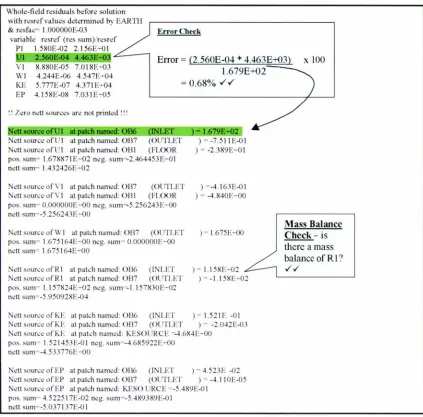
Figure 3-2 Example Output from PHOENICS - Steady-state Simulation ---65

Figure 3-3 PHOENICS Result file from a steady-state simulation ---66

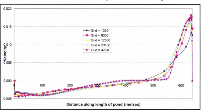
Figure 3-4 Grid Comparison, Velocity Plot, Case 1---69

Figure 3-5 Grid Comparison, Coliform Plot, Case 1 ---69

Figure 3-7 Grid Comparison, Coliform Plot, Case 2 --- 70

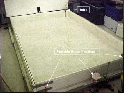
Figure 3-8 Laboratory model--- 73

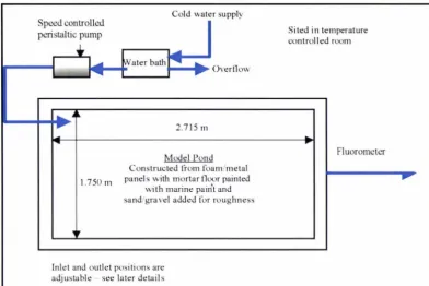
Figure 3-9 Experimental Set-up - Laboratory Pond (Shilton 2001, pg 78)--- 76

Figure 3-10 Set-up of Tracer Study on Laboratory pond --- 77

Figure 3-11 Map of Ashhurst showing pond location--- 78

Figure 3-12 Ashhurst secondary pond --- 79

Figure 3-13 Schematic diagram of existing Ashhurst secondary pond---79

Figure 3-14 Fabricated insert for field trial -Ashhurst ( diagram not to scale) ---80

Figure 3-15 Schematic Layout - Ashhurst Field Trial 2 (diagram not to scale)---80

Figure 3-16 Fabricated insert for inlet, second Ashhurst field trial ---81

Figure 3-17 Schematic Diagram of Baffie---81

Figure 4-1 Flow Pattern Case 1 (basic pond)---86

Figure 4-2 Coli form Concentration Case 1 (basic pond) ---86

Figure 4-3 Flow Pattern Case 2 (traditional two baffie case)---88

Figure 4-4 Coliform Concentration Case 2 (traditional two baffie case)---88

Figure 4-5 Comparison of Outlet Velocities Case 1 - Basic Case (left) and Case 2 (right) --- --- ---- --- --- --- --- --- 8 9 Figure 4-6 Flow Pattern Case 3 (traditional four baffie case) ---90

Figure 4-7 Channelling due to 90% width baffies (Watters et al., 1973, pg 49) ---90

Figure 4-8 Coliform concentration profile - Case 3 (traditional four baffie case) ---91

Figure 4-9 Flow Pattern Case 4 (traditional six baffie case )---92

Figure 4-10 Coliform Concentration Case 4 (traditional six baffle case) ---92

Figure 4-11 Flow Pattern Case 5 (traditional eight baffie case)---94

Figure 4-12 Coliform Concentration Profile Case 5 (traditional eight baffie case)--94

Figure 4-13 Flow Pattern Case 6 (two baffies evenly spaced)---96

Figure 4-14 Coliform Concentration Case 6 (two baffies, evenly spaced)---97

Figure 4-15 Flow Pattern Case 7 (single central baffie) ---98

Figure 4-16 Coliform Concentration Case 7 ( single central baffle) ---99

Figure 4-17 Flow Pattern Case 8 (single baffle, inlet end) --- 100

Figure 4-18 Coliform Concentration Case 8 (single baffle, inlet end)--- 101

Figure 4-19 Flow Pattern Case 9 (single baffle, outlet end)--- 102

Figure 4-20 Flow Pattern Case 10 (single baffle, outlet end)--- 102

Figure 4-22 Coliform Concentration Case 10 (single baffle, outlet end) --- 103 Figure 4-23 Flow Pattern Case 11 (single baffle, outlet end, outlet moved)--- 105 Figure 4-24 Coliform Concentration Case 11 (single baffle, outlet end, outlet moved)

--- 105 Figure 4-25 Flow Pattern Case 12 ( central wall with middle opening) --- 107 Figure 4-26 Coliform Concentration Case 12 ( central wall with middle opening) 107 Figure 4-27 Flow Pattern Case 13 (two stub baflles)--- 109 Figure 4-28 Coliform Concentration Case 13 (two stub baflles) --- 109 Figure 4-29 Enlargement oflnlet Comer of Case 13--- 1 I 0 Figure 4-30 Flow Pattern Case 14 (two stub baflles, outlet moved}--- 111 Figure 4-31 Coliform Concentration Case 14 (two stub baflles, outlet moved)---- 112 Figure 4-32 Flow Pattern Case 15 (two standard baffles, outlet moved)--- 113 Figure 4-33 Coliform Concentration Case 15 (two standard baffles, outlet moved)

---114 Figure 4-34 Comparison of velocity vectors: Case 14 and Case 15, yellow lines

indicate extent of higher velocity area --- 114 Figure 4-3 5 Flow Pattern Case 16 ( one stub baflle )--- I 15 Figure 4-36 Coliform Concentration Profile Case 16 (one stub baflle)--- 116 Figure 4-3 7 Case 17 (vertical inlet) -Coliform profile, arrows indicating circulation

direction --- --- --- I 18 Figure 4-3 8 Flow Pattern Case 18 ( diffuse inlet) --- 119 Figure 4-3 9 Coli form Concentration Case 18 ( diffuse inlet) --- 120

Figure 5-1 Full Tracer Study Results - Base Case (Shilton, 2001) --- 129 Figure 5-2 Tracer Study Results - Base Case, First 120 minutes (Shilton 2001 )--- 130 Figure 5-3 Dye flow path - Lab Tracer Study Case L2 --- 131 Figure 5-4 Tracer Study Results Case L2 (traditional two baffle case) --- 132

Figure 5-5 Comparison Plot - CFD & Laboratory Tracer Studies, Case L2--- 133 Figure 5-6 Dye Flow Path -Lab Tracer Study Case L4 (traditional six baflle case)

--- 135 Figure 5-7 Slug of Dye, Case L4 (traditional six baflle case)--- 136 Figure 5-8 Full Tracer Study Results Case L4 (traditional six baflle case)--- 136 Figure 5-9 Comparison HRT -Case L2 (traditional two baflle) and Case L4

Figure 5-10 Cell flow pattern, showing channelling, Case L4 --- 138

Figure 5-11 Currents caused by 90% width baffies (Watters et al., 1973, pg 49) - 138 Figure 5-12 Cells of Case L2, showing they are well-mixed--- 13 9 Figure 5-13 Comparison Plot - CFO and Laboratory Tracer Studies, Case L4 ---- 139

Figure 5-14 Dye Flow Pattern Lab Tracer Study Case Ll 1 --- 141

Figure 5-15 Full Tracer Study Results Case L 11 --- 142

Figure 5-16 Comparison HRT - Case L2 (traditional two baffie) and Case Ll 1 (single baffle, outlet end, outlet moved), first 120 minutes--- 143

Figure 5-17 Comparison plot - CFO and Laboratory results, Case L 11--- 144

Figure 5-18 Dye Flow Pattern - Case L 14 Laboratory tracer study --- 145

Figure 5-I 9 Tracer study results Case L 14 ( two stub baffies, outlet moved)--- 146

Figure 5-20 Comparison HRT of Case L2 (traditional two baffle) and Case Ll4 (two stub baffies, outlet moved) --- 14 7 Figure 5-21 Comparison Plot - CFO and Laboratory Tracer Studies, Case L 14 --- 148

Figure 5-22 Outlet end of Case LIS (two long baffies, outlet moved) showing chann e

11 i

Figure 5-24 Comparison HRT of Case Ll4 (two stub baffles, outlet moved) and Case L 15 (two long baffies, outlet moved)--- 151

Figure 5-25 Lab and CFO Tracer study results Case L 15 (two long baffles, outlet moved) --- 1 5 2 Figure 5-26 Dye flow pattern - Case L 17 ( vertical inlet) --- 153

Figure 5-2 7 Full Tracer Study Results Case L 17 ( vertical inlet)--- 154

Figure 5-28Comparison Plot of Laboratory Results - Basic Case (Run 9, Shilton, 2001) and Case L 11 --- 156

Figure 5-29 Comparison Plot of CFO Results - Basic Case (Run 9, Shilton, 2001) and Case L 11--- 157

Figure 6-1 Ashhurst secondary pond--- 159

Figure 6-2 Auto-sampler set-up at outlet - Ashhurst pond--- 160

Figure 6-3 Tracer welling up from vertical inlet - Ashhurst Field Trial 1 --- 161

Figure 6-4 Dye movement - Ashhurst Field Trial 1 --- 161

Figure 6-5 Diagram depicting dye movement - Ashhurst Field Trial 1 --- 162

Figure 6-7 Comparison HR T plot - normal & vertical inlet, Ashhurst --- 163

Figure 6-8 Comparison HRT Curve - normal & vertical inlet, Ashhurst - first portion of tracer run --- 163

Figure 6-9 Flow pattern at Floor Level in Water Reservoir (Shi lton et al., 2000a, pg 7) --- 165

Figure 6-10 Case AshA - Unmodified Ashhurst Pond--- 166

Figure 6-1 1 Cases AshB and AshC - two stub bail es --- 16 7 Figure 6-12 Cases AshD to AshG - Two stub baffle, inlet turned. --- 168

Figure 6-13 Cases Ash to AshJ - Inlet Manipulation--- 169

Figure 6-14 Flow Pattern - Case Ashl --- 169

Figure 6-15 Case AshK - Combination of turned inlet and stub baile --- 170

Figure 6-16 Cases AshL and AshM - Manipulations of Case AshK --- 171

Figure 6-17 Cases AshN to AshR - Central Outlet Investigations--- 172

Figure 6-18 Case AshS - Vertical Inlet plus Bailes--- 173

Figure 6-19 Case AshT - Standard length, evenly spaced baffles--- 174

Figure 6-20 Second Field Trial Design -Ashhurst Pond --- 174

Figure 6-21 Second monitoring point - second field trial--- 175

Figure 6-22 Dye flow pattern, Field Trial 2 --- 175

Figure 6-23 Dimensionless tracer study results - Field Trial 2, main outlet and baffle outlet, full data--- I 77 Figure 6-24 Dimensionless tracer study results - Field Trial 2, main outlet, initial data --- I 7 7 Figure 6-25 Comparison Plot - Field Trial 2 and Un-modified Pond--- 178

Figure 6-26 Comparison Plot - Field Trial 2 and Un-modified Pond, initial data-- 179

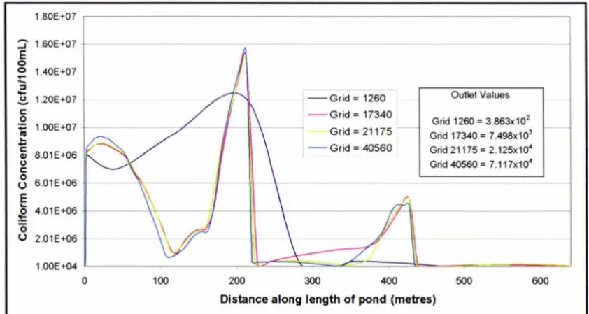
Figure 6-27 Comparison plot - CFD and actual results, main outlet, Field Trial 2 180 Figure 6-28 Comparison plot - CFO results, main and baffie outlets, Field Trial 2 181 Figure 7-1 Number of Baffles versus Coliform Concentration at outlet--- 184

Figure 7-2 Flow pattern within each cell, 6 baflle case (Case 4) --- 193

Figure 7-3 Channelling caused by 90% width baffles (Watters eta/., 1973)--- 193

Figure 7-4 Outlet end of Case 15 (two long baffles, outlet moved) showing channel Ii ng pattern --- 194

Figure 7-6 Ashhurst model, inlet turned into side wall --- 196 Figure 7-7 Ashhurst, inlet turned back to wall, 14m baffle located l /3 length from

end wal 1--- 1 97

TABLE OF TABLES

1.

INTRODUCTION

This section will briefly introduce the need for the research, and the objectives and approach of the work.

1.1

The Need for the Research

Waste stabilisation ponds are a common technology used for treating domestic, agricultural and industrial wastewaters. They are common in New Zealand, but are

also a low-cost, low-technology application for wastewater treatment in developing countries.

The overall efficiency of these systems is dependent on a number of factors. Watters

( 1971) cites biological factors as having been considered the most important, and hydraulic factors were given little attention. Over recent years, research has given more importance to hydraulic factors.

Hydraulic flow characteristics such as bulk flow patterns, short-circuiting, inlet and outlet positioning, presence of 'dead spaces' and the use of baffles are of significant importance to the overall efficiency of a pond system. Baffles can offer such improvements if properly designed. They can direct flow in such a way as to reduce hydraulic short-circuiting and the presence of dead spaces.

There are a great number of ponds used in New Zealand and throughout the world. These existing ponds are likely to be suffering from poor hydraulic, and therefore, treatment efficiency. This lack of efficiency can give ponds a bad reputation.

1.2

Objectives and Approach

The aim of this research was to contribute to the improved understanding of baffle design and use in waste stabilisation ponds. The use of computational fluid dynamics (CFO) modelling as a design tool was also evaluated. The specific objectives of the thesis are given below:

• To investigate the use of baffles in waste stabilisation ponds in terms of: o Length of baffles

o Number ofbaffies o Position of baffles

• To investigate the effect of inlet type, and outlet position

• To evaluate the use of CFO as a design tool to investigate various baffle configurations

• To apply the findings of the work into the field environment

To achieve the given objectives, the work was completed in three phases. In the first phase of work, a range of pond configurations was tested within the CFO environment. This produced an idea of the hydraulic and treatment efficiency of each configuration and allowed a large range of designs to be tested in a timely manner. The time and cost involved with laboratory models and field studies can often be prohibitive.

The second phase of the work involved taking some well-performing configurations from the CFD environment and testing them in a laboratory model pond. The use of CFD modelling as a design tool is relatively new to the field of waste stabilisation ponds, therefore the comparison between the CFO results and a traditional testing

method was beneficial.

2.

2.1

Waste Stabilisation Ponds

Waste stabilisation ponds ( oxidation ponds, lagoons) are relatively shallow bodies of wastewater contained in an earthen basin (Metcalf & Eddy, 1991 ). The technology is well-used and the reasons for this are summarised by Shelef & Kanarek (1995), and Mara et al., ( 1992a):

Advantages

o Low capital investment, especially with regard to construction cost

o Simple flow scheme, equipment and installation (minimum of p1pmg, pumping, aeration, and reduced need for pre-treatment)

o Low energy and operating costs o Simplicity of operation

o Relatively high and consistent level of treatment due to long retention time, biological competition and settling

o Buffering of peak hydraulic loads

o Relative resistance to shock organic loads, therefore suited to summer tourist locations with higher temperatures providing raised treatment efficiency and the ability to allow increased loading

o Sludge digestion is incorporated into treatment, particularly with the use of anaerobic ponds

o Some 'ultimate disposal' due to evaporation and seepage (unlined ponds) o Some nutrient removal

o Algal harvesting (high-rate ponds) o Effluent storage for reuse by irrigation

Disadvantages

o High land area requirements

o Effluent can contain high suspended algal concentrations, the disposal of which to receiving bodies is controversial

o Overloading or abrupt climatic changes can cause odour nuisances and

deterioration of effiuent quality

o Possibility of groundwater contamination by seepage from ponds

o Water losses due to evaporation and seepage in situations where water for

reuse is considered an important commodity

These lists are comprehensive, although to some extent, the disadvantages listed above can be reduced. For example, by lining a pond the problem of seepage and the possibility of groundwater contamination can be removed. Also the use of anaerobic ponds at the front end of a pond system can reduce the land area required.

Wood (1997) stated that the continued use of pond technology is being undermined by the inconsistent performance relative to current discharge requirements, particularly with respect to suspended solids, pathogen, and nutrien t removal. As the public grows more aware of the issues relating to the protection and sustainability of our natural environment, the regulations governing such issues become more stringent. Craggs ( I 998) also commented on the declining popularity of pond systems due to the demand for consistent and high quality discharges. Fritz et al., (1979) reports that waste stabilisation ponds have "fallen into disfavour" (pg. 2724) due to high land requirements, high orgamc concentrations in effiuent and dependence on environmental factors.

Fritz et al., ( 1979) noted that many of the problems, as mentioned above, result from a lack of understanding of the basic biomechanical mechanisms involved in ponds, improper operation and system overloading. Wood (1997) commented on the apparent simplicity of ponds and how it can be deceiving, " ... for their performance in removing pollutants is a complex function of fluid hydrodynamics, the contacting

of biomass with pollutants, physico-chemical and biological mechanisms. "(pg. 2).

As has been shown, waste stabilisation ponds have a large number of advantages

developing areas where the infrastructure and expertise is not available to support

them.

Research needs to be carried out into the reasons for poor performance of existing

ponds and into the development of new pond designs.

2.2

Types of Ponds

The classification of ponds is usually based on the nature of the biological activity

within the pond -aerobic, anaerobic, or facultative. An anaerobic pond when used, is

the first pond in a series and is termed a primary pond. Aerobic ponds can be termed

primary or secondary ponds depending on whether it follows an anaerobic pond.

Facultative ponds have an anaerobic zone on the bottom, with the aerobic zone near

the surface. Maturation ponds and high rate algal ponds are also discussed.

2.2.1. Anaerobic

Anaerobic ponds when used, are the first ponds in a series. They receive the highest

organic loading and their purpose is to remove the bulk of this organic load. Their

depth is in the range of 2-Sm in order to accommodate the accumulation of sludge.

The depth also maintains anaerobic conditions by reducing the surface area to

volume ratio (Mara et al., 1992a).

The treatment performance of an anaerobic pond is highly dependent on temperature,

with the critical temperature for methanogenesis about 10°C. Below this temperature

minimal sludge digestion occurs and the pond acts more as a settlement pond. In

warmer climates therefore, anaerobic ponds are particularly effective. Mara et al.,

(1992a) mention that in temperatures above 20°C, 60% of the BOD (biochemical

oxygen demand) can be removed in a pond with a one day retention time.

A typical problem with the existence and operation of anaerobic ponds is the

potential for objectionable odours due to fermentation processes (hydrogen sulphide

and other volatile by-products). Many district and regional councils in New Zealand

make mention of "offensive or objectionable odours" within various rules and

that of the public. According to Meiring et al., 1968 (in Curtis and Mara, 1994), control of odour can be achieved by ensuring organic loads of less than 400g/m 3 d as long as the incoming sewage has a sulphate concentration of less than 500mg/L. Normal domestic or municipal wastewaters contain less than 300mg sulphate/L

(Mara & Pearson 1998).

A novel application of anaerobic pond technology is within the Advanced lntegrated Wastewater Pond System (AIWPS) developed during more than 35 years of pond research at the University of California at Berkley by Oswald and co-workers (Craggs et al., 1998). As part of the AIWPS system, Oswald et al., ( 1994) investigated the use of fermentation pits within a primary facultative pond. These pits are semi-enclosed in the anaerobic bottom layer of a deep facultative pond. The

semi-enclosed nature prevents oxygenated water from the aerobic layer entering the pit and helps prevent odour escaping

2.2.2. Facultative

Facultative ponds are the most common type of pond in use throughout the world.

There are two types: primary - which receive raw wastewater, and secondary

-which receive settled wastewater, often from a front end anaerobic pond. Pelczar et al., ( 1993) define facultative anaerobes as organisms that do not require oxygen for growth (but may use it if available), which grow well under both aerobic and

anaerobic conditions, and for which oxygen is not toxic.

Facultative ponds are designed to remove BOD on a surface loading basis of

100-400 kg BOD/ha.d (Mara et al., 1992a). The loading of a facultative pond is lower than that of an anaerobic pond. High removal of pathogens is also seen in facultative ponds (Mara et al., 1992b ).

The lower layer of a facultative pond acts in a manner similar to that of an anaerob ic pond, as shown in Figure 2-1. It has a sludge layer below an anoxic water layer. The upper reaches of the pond are aerobic due to diffusion of oxygen from the atmosphere and the presence of oxygen-producing algae. The presence of the algae

the ponds become overloaded they may appear red or pink due to the presence of anaerobic purple sulphide-oxidising photosynthetic bacteria (Mara et al., 1992a).

Wind (wind ocllon promotes mixing and reoeration)

Reoerohon Wastewater

~

solids

Bollom

sludge'::---Organic wastes ---,..

o,

(during daylight hours}

Sunlight

0

/.//

co,

++t

_t

_l

r

t

t

If o,ygen is not present in upper layers of pond, odorous gases con be released

I

Aerobic zone

Focultotive zone

+

-Organic acids, ____. co

2 + NH3 + H2S + CH4

alcohols Anaerobic zone

Figure 2-1 Facultative Pond (Tchobanoglous and Schroeder, 1985, pg 635)

2.2.3. Maturation Ponds

Maturation ponds are predominantly designed to achieve pathogen removal. They are typically aerobic throughout their depth (I-I .Sm). Their BOD removal is quite small, but their contribution to nitrogen and phosphorus removal can be significant (Mara et al., 1992a).

Pathogen die-off is promoted by the high pH levels generated in the ponds (Mara et al., 1992b), with reductions of 4-6 log units of faecal coliforms, 2-4 log units for

faecal viruses. Curtis and Mara ( 1994) categorises the mechanisms by which

pathogens are removed from ponds: the dark mechanisms, pH, and light. Dark mechanisms are those of starvation (due to lack of nutrients), predation (by protozoa)

and enteric bacteria binding to algae. In regard to pH, Escherichia coli are known to

require a neutral pH, therefore an increase in pH can rapidly kill the bacterial cells. With respect to light - the energy in sunlight is transferred to bacterial and viral cells in such a manner as to cause parts of the cell or virus to be destroyed. Curtis and

2.2.4. High-Rate Algal Ponds

High-rate algal ponds were developed at the University of California (USA) by Oswald and co-workers (Shelef and Azov, 1987). High-rate algal ponds are usually 'race track' shaped and are mixed with a paddle wheel. High-rate algal ponds are shallower than conventional facultative ponds, but require a much shorter retention time and produce far more dissolved oxygen (Green et al., 1996). As reported by Green et al., (1996) a well-designed high-rate algal pond will generate high amounts

of dissolved oxygen per unit area.

Another advantage of such systems is the harvesting and processing of the algal-bacterial biomass to produce potentially valuable proteinaceous animal feed that may be needed where feed shortages may occur (Shelef and Azov 1987). This however is not an issue in New Zealand due to readily available protein sources.

These systems have been researched extensively in recent times, with a number of

papers presented at the 5th IW A Specialist Conference on Waste Stabilisation Ponds held in Auckland, New Zealand, 2002. They included Chen et al., (2002); Craggs et al., (2002a & 2002b); Cromar & Fallowfield (2002); da Costa et al., (2002); El Hamouri et al., (2002); and Jupsin et al., (2002).

2.3

Pond Design

There are a number of alternative approaches to the design of waste stabilisation

ponds, these include: o Loading Rates

o Empirical Design Equations o Rational Models

o Mechanistic Modelling

2.3.1. Loading Rates

In the loading rate approach, parameters such as flow, population, or BOD loading

BOD5/ha.d as the design loading for raw sewage ponds and secondary ponds (MWD 1974). This type of approach ignores the effects of pond shape, wastewater

characteristics, temperature and so on.

Recent design guidelines (Mara & Pearson 1998, Mara

et al

.,

equations based on loading rates which take into account the effect of temperature on

the performance of various pond types (anaerobic, facultative and maturation).

With respect to maturation ponds, Mara & Pearson ( 1998) suggest a mm1mum

acceptable retention time of 3 days (4-5 days for temperatures below 20°C). The

reason for this is to minimize hydraulic short-circuiting and prevent algal washout.

The basis for this arbitrary value and the reasoning is not given.

The loading rate approach to pond design essentially treats a pond as a 'black box'

and while temperature effects are taken into account, many other aspects of pond

performance - shape for example - are largely ignored.

2.3.2. Empirical Design Equations

Empirical design equations are derived from regression of experimental pond

performance data. Design approaches include areal loading, the McGarry and Pescod

relationship, Bucksteeg recommendations, Gloyna equation and the Larson Relation

(Wood 1997).

As this method involves the regression of data for one particular pond or a series of

ponds the question is raised as to how applicable the equations will be in other

locations. Prats and Llavador (1994) and Wood (1997) reported that as correlations

are based on data collected from selected sites or locations, the validity of this

method when applied to other different sites is debatable.

2.3.3. Rational Models

This design approach uses theory developed in the field of reactor engineering. First

regimes ideal and non-ideal. Attempts have also been made to produce a combined model incorporating both flow regimes.

2.3.3.1. Ideal Flow

Ideal flow is a theoretical concept for which zero mixing (plug-flow) or infinite mixing ( completely mixed flow) is assumed. Both types of ideal flows have been used to describe waste stabilisation pond systems.

Plug flow assumes no diffusion or mixing of the substrate occurs in the reactor, or pond in this application. Essentially, this means that the incoming wastewater travels as a slug from the inlet to the outlet. The integrated rate equation is as follows:

C 'C e-kt

i i

where C~ = effiuent concentration (mg/L)

C

k first order reaction rate constant (1/d) t time (d)

Middlebrooks ( 1987) conducted an investigation to evaluate the most frequently used design equations. He found that the first order plug flow model gave the best fit of all the rational models. As reported by Wood ( 1997), "while the plug flow is a simple model being applied to a complex system, it is often superior to a multi-parameter model with several undetermined coefficients." (pg. 25)

At the other extreme, completely mixed flow assumes the substrate is instantaneously mixed upon entering the reactor. For this mixing regime the CSTR (completely stirred tank reactor) equation can be derived:

Ce/C

=

C/Ci

where n number of ponds in series

There are limitations to assuming 'ideal' conditions with regard to the flow within waste stabilisation ponds. "The accuracy of these equations may vary substantially with actual pond conditions and therefore their application is limited" (Preul and Wagner 1987, pg. 206).

2.3.3.2. Non-Ideal !·low

In reality, flow through reactors and waste stabilisation ponds will exist somewhere between the two extremes of plug flow and completely mixed flow. This is termed non-ideal flow.

Thirumurthi ( 1969) concluded from studies on design principles for waste stabilisation ponds, that the Wehner-Withem equation is a basic tool suitable for design.

Wehner and Wilhelm ( 1956) presented an analysis of the boundary conditions for a steady-state flow reactor with first order reaction kinetics and axial diffusion The equation they derived is valid for reactors with any kind of entry or exit configurations. The common fom1 of the equation is given below:

where d = O/uL (dispersion number) a= ,/1

+

Ce, Ci= effluent and influent substrate concentrations D = axial dispersion co-efficient (m2 /h)

u = fluid velocity (m/h) L = characteristic length (m)

k = first order reaction constant (1/h) t = detention time (h)

Thirumurthi (1969) further simplified the equation by neglecting the second term in the denominator:

The error involved in neglecting the second term of the equation is not significant until the value of the dispersion number exceeds two. After this point the error may be significant, however Thirumurthi (1969) noted that due to the low hydraulic loads the value of the dispersion number is unlikely to exceed one in waste stabilisation ponds.

In the conclusion to an investigation into the use of the Wehner-Wilhelm equation, Polpraset and Bhattarai ( 1985) stated "It was found that this equation could perform with a high degree of accuracy in the prediction of the total and faecal coliform die-off; and the results obtained had significantly higher correlation coefficient values than those of the completely mixed equations" (pg. 56 ).

2.3.3.3. Comhined Pondlvfodels

Models have been developed combining plug, completely mixed and dispersed flow. ln these models the pond is considered as a number of separate but interconnected flow regions with flow exchange between them.

c)-r

Q

lJ

L~

r

I

F C

(al Given now situ:uion

Q

r

I

(b) Finite :-.1agc: modd

F a

Figure 2-2 Finite Stage Model (Watters et al., 1973, pg 16)

The use of combined pond models has produced good model fits, however, the

method is not predictive. Parameters used in these models need to be calculated

using experimental data. Ferrara and Harleman ( 1981) noted that the input parameter

values needed by these models cannot be reliably predicted at this time.

2.3.4. Mechanistic Modelling

According to Colomer and Rico (1993 ), the application of a mechanistic model for a

pond system consists of "considering a biological reactor and applying a complete

material balance, including terms for substances produced or consumed, inflow,

outflow, and accumulation for each component. Resolving simultaneously the

system differential equations for all components, the evolution of each one with the

time is obtained." (pg. 679). Two of the significant investigations on mechanistic

modelling were carried out by Fritz

et al.

, (1979)

Rico

Fritz

et al

.

, (1979)

reviewing existing models describing the behaviour of pond systems the following

performance based on the variety of physical and biochemical factors that govern the

quality of pond effluents." (pg. 2 725). The authors go on to say that non-steady-state

simulations of biomass and biochemical species whose kinetics are dependent on

environmental factors have not previously been performed. The model proposed by

Fritz et al., (1979) consisted of twelve mass balance equations for biochemical and biomass components. Figure 2-3 below shows a schematic diagram of the processes

occurring in a pond ecosystem.

-

_/!I

_ll

---

Wind

-

_I/I

_l

_l

-

_~

lntcrlaci~I

Figure 2-3 Schematic diagram of 11rocesscs in a tlond ecosystem (Fritz et al., 1993, pg 2725)

The model as developed gave some reasonable results, however the authors listed a

series of conclusions and recommendations highlighting areas for further

development to improve the model.

Colomer and Rico (1993) proposed a revision to the Fritz et al., (1979) model which

was then tested against a set of field data. The authors concluded that the revised

model "provides values in the same order of magnitude as real data, and it

reproduces reasonably well the variaions registered." (Colomer and Rico, 1993, pg.

Fritz et al., (1979) model and that the calculated concentrations of effiuent depend significantly on the influent characteristics. The processes within the pond contribute less to the calculations.

2.4

Importance of Pond Hydraulics

The performance of ponds has been said to be largely dependent on climatic conditions. Kilani and Ogunrombi ( 1984) stated that hydraulic flow pattern rn stabilisation ponds is one of the major factors influencing pond performance. A thorough knowledge of the hydraulic characterisations in ponds would seem important for efficient and more appropriate pond design.

Wood ( 1997) stated that the pond hydraulics is often the limiting factor in achieving high pond performance, while Thirumurthi ( 1969) outlined that little attention had been given to pond shape, presence of dead spaces, inlet/outlet flow patterns.

Watters et al., ( 1973) stated that little attention had been given in the past to the hydraulic characteristics of waste stabilisation ponds. Particular reference was given to the gross flow patterns within ponds which are affected by the shape of the lagoon, presence of dead spaces, existence of density differences, and the positioning of inlets and outlets. They concluded from their research that the pond hydraulics are important in determining the treatment efficiency of that pond. Hydraulic factors should be considered to maximise economy of construction and operation for maximum treatment.

o The mam axis of flow should not be aligned with the prevailing wind

direction.

o Ponds should be located a distance away from any element that may shield a

pond from the mixing effect of wind.

o The simplest measure to avoid short-circuiting in ponds is to avoid locating

inlet and outlets close together.

o Multiple inlets and outlets as well as the use of diffusers have proved useful

in the prevention of short-circuiting.

o The shape of the ponds should be rectangular with rounded comers. Other

shapes (branching, kidney, circular) have been shown to result in a higher

degree of short-circuiting.

o The use of baffles improves performance. However, this measure results in a

considerable increase in the cost of ponds.

Moreno (1990) commented that the performance of stabilisation ponds can be

improved substantially through simple and economical measures to correct

circulation patterns inside ponds. Also, while it would be far better to consider

hydraulic implications during the design process, it is feasible to improve the

hydraulics of existing ponds.

Wood (1997) in his doctorate thesis on the development of computational fluid

dynamics models for the design of waste stabilisation ponds made some interesting

comments. Mention was made that the factors which influence the hydraulics of

ponds are well known, however the relative importance of these factors (wind,

thermal energy, geometry, inlet design & baffles) is poorly quantified. This reduces

pond design to an art form, relying more on experience than the application of the

fundamental phenomena involved. Also, while small-scale experimental studies

provide an economic evaluation of pond designs, scale-up issues are often a

hindrance.

Shilton (2001) concluded that despite the research he reviewed, the insight into pond

hydraulic behaviour is poor in the majority of the studies consisting of stimulus

has retarded efforts to improve and optimise hydraulic and treatment efficiency at a practical design level.

Hydraulic efficiency is usually expressed in terms of the approximation to plug-flow, the amount of the pond that is utilised - or volume of dead space, the time taken for a peak of tracer to reach the outlet, or mean hydraulic residence time. As mentioned by many pieces of research, dead spaces usually occur in the corners of rectangular ponds, where the major water flow bypasses these areas and back-eddies are often formed.

2.5

Factors Affecting Pond Hydraulics

In this section, the factors affecting the hydraulics of ponds will be discussed, in particular: inlet/outlet configuration, wind, and stratification. Baffles are also a significant factor that can affect pond hydraulics and form a major part of the research for this thesis, and will be discussed in detail in Section 2.6.

2.5.1. Inlets/Outlet Configuration

Mention has been made by several researchers about the influence of inlet/outlet configuration on the hydraulics of a pond, but there have been few significant bodies of work that have investigated different configurations. Mara and Pearson ( 1998) stated: "A single inlet and outlet are usually sufficient. These should be located in diagonally opposite comers of the pond (the inlet should not discharge centrally in

the pond as this maximises hydraulic short-circuiting). The use of complicated multi-inlet and multi-outlet designs is unnecessary and not recommended." (pg. 59). The statement above appears to have been based on available knowledge at the time. It has been seen since noted in further research that the inlet/outlet positions require careful thought on a site-by-site basis.

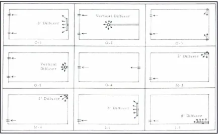
Watters et al., (1973) used a scale model pond in a laboratory to investigate the

effect of nine different inlet/outlet positions and designs (including various diffusers)

on hydraulic and treatment efficiency. They are shown in Figure 2-4 below.

·

-

_'

-

+

d' Diik scr

=I

--~

..

...

f

-'

-

-

0-1 0-2 0-)

==-!-

-

_I

I

2' Dll!Jscr ",1"-f

Vert1C'c1l

*

t::-

+-0 -5 0-4 M 3

·-~1 D1:11.1:;cr ... ..,...,

I

j

I

I

d 01! 1 1:.i.: r _I

3' D1ftuscr

= ~

-

_c=-

,\!-4 l-1 :

Figure 2-4 Inlet/Outlet Configuration tested b~· Watters et al., (1973, pg 41)

Their research utilised tracer studies from which the concentration-versus-time

curves could be used to calculate various hydraulic parameters. These curves were

also combined with the first order reaction equation to determine treatment

efficiency.

In their conclusions, they stated that the inlet and outlet types and configurations had

a significant effect on the hydraulic characteristics and subsequent treatment

efficiency determinations. A change of as much of 42% was indicated by the data for

the important hydraulic parameters, while a change of 19% in treatment efficiency

was indicated for the two extreme conditions of inlets and outlets.

The inlet/outlet configurations tested by Watters et al., (1973) appear to have been

arbitrarily chosen without taking into account the flow pattern that may form from

the placing of the inlet. That is, they have not been chosen on the basis of what flow

configuration of an existing pond was known to produce a slow circulation pattern with a significant dead space in one corner then the best place for the outlet may be in that dead space.

Persson (2000) conducted a study usrng two-dimensional, vertically integrated numerical models to simulate hydraulic performance in 13 different pond layouts, including 5 with the same basic layout but differing inlets and outlets. The configurations tested are shown in Figure 2-5.

AL

_i

rrLfJ

of

t

sf

₊

Hf}

l

p 70 I

ct:=)

-f

+

Q

-El

+

DL

_J

-K

+

I

E ~

f

i,J

Figure 2-5 Configurations tested b~ Persson (2000)

0.1 . . - - - ,

009

- - - !

0.08

- - - !

i ~::

j

- - - !

I.I

i

u 0.03 - i - - - 1 c - - - + - - - c - - T - - - t 0.02 +----'-+--,,-+-_,._.. _ _ _ _ _ _ _ _ _ - - I

0.01 t - - - t - . . . , , . ~ ' - - - " - : : : - ~ - - - 1

0 ..L....L ___

t/tn

Figure 2-6 RTD Curves for Configurations B, Q, P, E (Persson, 2000, p246)

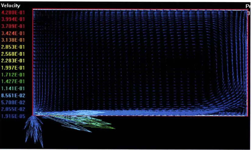
Shilton (2001) carried out investigations into the effect of outlet position, and into the effect of inlet type and position. With regard to the position of the outlet, it was observed that the outlet has minimal influence on the circulation pattern in the pond. The position of the outlet does change the overall flow pattern.

From his inlet investigations, Shilton (2001) also found the flow patterns of large and small horizontal inlets to be similar - except for the time lag due to the relative velocities produced by a large diameter inlet compared with a small diameter inlet The most interesting result however was the investigation into an up-turned vertical inlet When the pond had a horizontal inlet, a swirling pattern was produced in the pond - this led to short-circuiting. When the pond had an up -turned inlet, there was no swirling flow pattern produced and therefore short-circuiting was subsequently reduced.

I

inlet

+

+

_*

,.

A

_B

_C

1.:

w

I

+

,,

1,

outlet _{outlet outlet}

Figure 2-7 Inlet/Outlet Configurations tested by Fares et al., (1996, Fig.2)

Fares et al., (1996) concluded that the effect of the inlet/outlet arrangement only became significant at low wind speeds. A more thorough review of wind and its

correlation with inlet influences can be found in Section 2.5.2 of this thesis.

Other authors have made mention of the importance of inlet/outlet position and design (Moreno, l 990) but have not specifically studied the effect of moving or redesigning inlets and outlets. This mention of the inlet/outlet importance is also

often made without supporting data.

2.5.2. Wind

The effect of wind is often mentioned in literature as an influencing factor on pond hydraulics. For example, Thackston et al., ( 1987) concluded that wind is an uncontrollable variable so basins should be designed for the worst-case scenario for wind speed and direction and geometry designed to resist wind effects. In particular, the outlet should be oriented towards the prevailing wind, and baffies should be used to force several changes in flow and direction. However there is an absence of extensive study exclusively on the effect of wind. As stated by Shilton (2001), despite being regarded as the dominant driving force of flow in ponds, the influence of wind has been poorly researched. Indeed, Marecos do Monte ( 1985) commented that the effect of wind, which influences mixing in ponds, is impossible to fully take

Shilton (2001) included wind as a variable in a CFD model of a field pond. The results of the model were not far removed from the model without wind, and indeed the actual field results closely matched both models. He also performed an analysis of the power input by wind versus the power input from the inlet. Shilt on (2001) concluded that the effect of wind may have been over-estimated and the effect of the inlet under-estimated and that under certain circumstances, the inlet could be sized to ensure that it dominates over wind as the driving factor for flow most of the time.

Other research has attempted to add the effect of wind into mathematical models: Fares & Lloyd (1995), Fares et al., (1996) and Wood (1997). However this did not include extensive validation against field data.

A study was performed on quantifying wind effects by Watters et al., (1973) at the Utah Water Research Laboratory. Their work involved the construction of a wind-water tunnel to simulate a wind over wind-water situation, to evaluate diffusion coefficients as functions of wind shear for both stratified and un-stratified ponds. It is unclear from the work how the results found would then be applied to a field pond situation, with variable wind speed and direction.

2.5.3. Stratification

"Stratification is the temperature induced separation of the pond into layers.'' (Shilton 200 I, pg. 45). The layers of a stratified pond will differ in temperature, dissolved oxygen concentration and redox measurements. The different dissolved oxygen levels will typically mean that the top layer is aerobic and the bottom layer is anoxic. Therefore, the biological and chemical characteristics of the two layers will be quite different.

Stratification in ponds may have a detrimental effect on the hydraulic behaviour of the system. An inflow to a pond could possibly travel in only the top or bottom layer of a stratified pond without mixing in to its full volume.

o Influent more dense than ambient fluid (summer time flows) o Influent of the same density as ambient fluid

o Influent less dense than ambient fluid

Their conclusions were that the degree of stratification had an influence on the hydraulic performance. "For an increase in the degree of stratification ... the influence on the hydraulic parameters and treatment efficiency depended on the type of stratification." (pg. 61 ). They found that when the density of the influent wa~reater than the density of the ambient fluid the hydraulic performance improved, when the density of the influent is less than the ambient fluid the hydraulic efficiency decreased.

Cavalcanti et al., (2001) noted that the surprisingly high dead space volume in their polishing ponds was possibly due to a warmer and lighter upper layer on the surface over the cooler and denser bottom layer. Therefore, short-circuiting may have been

occumng.

From their tracer studies, MacDonald & Ernst (1986) concluded that stratification was responsible for short-circuiting. This conclusion however, was based on the tracer output rather than actual measurements of tracer within the pond.

2.6

Baffles

Baffles are essentially obstacles placed in a flow-path to achieve better hydraulic, and in some applications, treatment efficiency. They have been used successfully in the water industry chlorine contact tanks, water reservoirs, and stormwater detention ponds. Their benefits in nutrient removal and as attached growth systems is

also recognised in the wastewater industry.

The use of baffles for the improvement of hydraulic and treatment efficiency in waste stabilisation ponds has formed a major part of the research for this thesis,

In this section the application and benefits of baffles will be discussed, with specific regard to waste stabilisation ponds. Baffie use in water reservoirs, chlorine contact tanks and other uses will be included.

2.6.1. Hydraulic Investigations of Baffle Implementation

Baffles are commonly used as an attempt to improve the hydraulic and treatment efficiency of a waste stabilisation pond. Studies have been performed on a number of different baffle configurations with the general consensus being that the more baffles there are, the closer the approximation to plug-flow and the better the pond performance. As said by Reynolds et al., (1975): "Baffles would also (in addition to acting as attached growth .systems) affect the hydraulic flow pattern of the system and should reduce short circuiting and improve mixing conditions. Unfortunately, little research has been conducted in this area." (pg. I 005).

Watters et al., (1973) performed 17 different tests on selected evenly spaced baffle arrangements. Tests were performed using four different lateral spacings, which corresponded to 2, 4, 6 & 8 baffles. These four spacings were tested using three lengths of baflles; they were 50%, 70% and 90% of the width of the pond. An example is shown below in Figure 2-8. This figure depicts a six-baffle case with the baffles extending 70% across the width of the pond.

Figure 2-8 Bame configuration tested by Watters et al., 1973

When the baffles extended 50% across the width of the pond, short-circuiting was discovered shown in Figure 2-9.

,...

/ ' _"

....

"

'-,,,

,,,

-

-

Figure 2-9 Short-circuiting caused by 50% width baffles- Watters et al., 1973

u

.

~

..-

- - -

- -

- - -

- -

- -

- - - -

- -

----,

;::i.

~

' '1/

~

li

CJ.2

-

50% width

90% width .

70% width

4 bames

C.L

v.; E /; -= . 'i J

W i.l / 3 = . ')0

2 bames

!he loll'er the c111Te, the lesser the de1•iatio11from plugfloll'- and there.fore the

better the hydmulic efficiency.

0. 3 0.4

Figure 2-10 Plot of number of baffles versus hydraulic 1>erformance (adapted from Watters et al., 1973, pg 4 7)

Tests were also performed on vertical baffling, where the flow takes an over-under

path. A plan of the vertical baffles set-up is shown in Figure 2-11. It is probable that

the vertical baffles were tested due to an expectation that fluid would mix well in

each compartment prior to moving to the next. However, the results from these tests

were not as good as for the horizontal lateral baflling. Reynolds et al., (1975) also