MoL 2017 18: Dynamic Epistemic Logic Models for Predicting the Cognitive Difficulty of the Deductive Mastermind Game

(1)

Difficulty of the Deductive Mastermind Game

MSc Thesis

(Afstudeerscriptie)

written by

Bonan Zhao

(born March 23rd, 1993 in Shandong, China)

under the supervision of Dr Jakub Szymanik and Iris van de Pol, and submitted to the Board of Examiners in partial fulfillment of the requirements for the degree of

MSc in Logic

at the Universiteit van Amsterdam.

Date of the public defense: Members of the Thesis Committee:

August 31, 2017 Prof Benedikt Loewe (chair)

(2)

Abstract

(3)

First of all, many thanks toward my dear supervisors Jakub and Iris. Jakub, you are the person that led me to the interdisciplinary study of logic and cognitive science, and thank you for all the meetings, discussions, lectures and conversations we had. Iris, I learned so much from you, from caring about asking the question to writing a clear sentence. I would also like to thank Lena, Fernando and Peter for being in my committee, and a special thanks to Peter van Emde Boas for your interest in my thesis project.

My study at the ILLC is possible because of the generous financial support from the Amsterdam Excellence Scholarship, and I am truly grateful to your support. Thank you Fenrong and Johan for introducing logic to me, and supported me to pursue my study in Amsterdam. And thank you Sonja for being my mentor and helping me clear my worries when I got confused or stressed during these two unforgettable years.

Of course, my life at the ILLC is a wonderful experience because of my friends here. The MoL gang gave me the warmest accompany I could ever find, taught me how to appreciate beer and coffee, and showed me the magic of cake and pasta. Amsterdam became a home to me because of you; thank you guys!

(4)

List of Tables

3.1 Boolean translations for 2-pin DMM feedbacks . . . 12

4.1 Summary of complexity measurements . . . 35

4.2 Elimination power of clues . . . 37

5.1 Regression results for four DEL measurements . . . 46

5.2 Summary for standard deviationσ of distinct values in each DEL measure-ment . . . 49

5.3 Regression results for unordered DEL structures . . . 50

5.4 Regression results for tableaux models on the old and new datasets . . . . 53

5.5 Comparing tableaux model with DEL measurements . . . 54

(7)

1.1 A DMM game item . . . 2

2.1 A complete Mastermind game won in 5 conjectures . . . 4

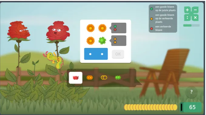
2.2 Screen shot of a DMM game item . . . 5

2.3 Ratings of 2-pin DMM game items . . . 8

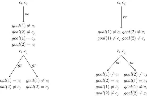
3.1 Branching rules for 2-pin DMM feedbacks . . . 13

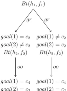
3.2 Two different decision trees for the same game item . . . 14

3.3 Tableaux tree for Example 3.2 . . . 15

3.4 Game item with four all gr feedbacks . . . 16

4.1 Illustration of the update sequence for Example 4.5 . . . 27

4.2 Screenshot of a 2-pin DMM game item . . . 32

4.3 Illustration of the update sequence for Example 4.8 . . . 33

4.4 Tableaux tree for the game item in Figure 4.7a . . . 40

4.5 A tree for DEL preconditions . . . 40

4.6 A tree for possible worlds . . . 41

4.7 Screenshots of two game items with gr-only feedbacks . . . 42

5.1 Plots for predictions and observed ratings of 2-pin game items . . . 48

5.3 Plots for default and unordered predictions . . . 50

5.4 Plots for DEL measurements that consider feedback types . . . 51

5.5 Plots for ratings of 2-pin game items . . . 53

1 The first 10 items from the raw dataset of 2-pin DMM game items . . . 64

(8)

Chapter 1 Introduction

“Don’t worry,” your friend tells you, “I heard the modal logic final will be easier than our weekly assignments.” In this situation, the difficulty of a logic question is evaluated by how hard it is for a student to solve it. How much time do you spend on it? How directly can you find the right answer? Do you indeed manage to find the right answer in the end? We call this the “cognitive difficulty” of the question or task at hand. We can study the cognitive difficulty of a variety of things such as solving a question in an exam, recognizing a color in a certain context, or interpreting the meaning of a quantifier in communication.

A fruitful method to study the cognitive difficulty of a task is to combine computa-tional and logical analyses. We can use logic to formalize a task into a computacomputa-tional problem, and then measure the complexity of this logic formalization as a predictor for the cognitive difficulty of this task. This two-staged method has proved useful in studying the cognitive difficulty of communicative and linguistic tasks, both theoretically (seeBerwick and Weinberg (1984); Cherniak (1986); Barton et al. (1987); Ristad (1993); Szymanik

(9)

[image:9.595.76.251.110.201.2]

Figure 1.1: A DMM game item

shows some available flowers that a player can choose to form her answer. The feedbacks provide information on the relationship between the flower sequence in a clue and the correct answer. DMM has been implemented in Math Garden, a popular on-line educational game system, which is used in pri-mary schools all over the Netherlands and has accu-mulated billions of behavioral data on how children play the games. Each DMM game item in Math Garden is associated with a rating of its difficulty, and this rating is computed based on children’s speed and accuracy in solving the game item. DMM is an ideal case study because (1) it can be naturally formalized using logic, and (2) it provides an empirical dataset on the cognitive difficulty of each game item, as indicated by the ratings. By for-malizing DMM with logic, we define complexity measures over such formalization, and use these measures as predictors for the cognitive difficulty of DMM game items. Therefore, this is a case study of using logic to capture cognitive difficulty.

Gierasimczuk et al.(2013) propose an analytical tableaux model of DMM that gives an account of the cognitive difficulty of a DMM game item based on the size of the decision tree generated for that item. Their analytic tableaux model correctly predicted 63% of the item ratings,1 _{but the model is challenged from different perspectives, which include the}

following: (1) The tableaux model is based on strong assumptions. The model assumes that players reason by cases and process feedbacks one by one, and Gierasimczuk et al.

(2013) assume that the size of tableaux decision trees is a proxy for working memory load. (2) The tableaux model is unable to capture certain observed reasoning patterns. The tableaux formalization is order-dependent. That is, a decision tree in this model can only unfold one clue after another, and therefore cannot represent cross-clue patterns. However, it has been observed that when the clues for a particular game item all contain green-red feedback, children can use this information to make a more strategic move than processing clues one by one (van der Maas, 2017). Consider Figure 1.1 where two green-red feedbacks are given. A child can deduce that the orange daisy that stands at the second place in each clue corresponds to the green feedback and shall go directly to the answer, and the flowers that stand in the first place in the clues correspond to the red feedback peg and therefore should not appear. The tableaux model cannot represent such a move. (3) Since the complexity measurements in the tableaux model are generated by the particular formalization, it is not clear whether they indeed capture the cognitive difficulty of the DMM game, or simply are some artifacts of the formalization itself.

1_{In the 2013 dataset, the tableaux model can predict up to 75% item ratings for 100 game items, and}

(10)

The above mentioned drawbacks hinder the tableaux formalization, and we want to design a different model that uses fewer assumptions, better represents the choices of the children, and can cross check the plausibility of the logic-based model. We used Dynamic Epistemic Logic (DEL) to build a new model of DMM. This model makes fewer assumptions than the tableaux model, because it does not require reasoning by cases and the way of finding solutions does not depend on the order in which piece of information are processed. The DEL model of DMM solves the game via a natural approach of eliminating impossible options and deliberating over possible answers, and it can give an account of the cross-clue pattern that is mentioned earlier. By testing complexity measurements of the DEL formalization against the empirical dataset, we showed that the DEL model can predict 66% of the item ratings, and thereby performs slightly better than the tableaux model based on the latest dataset. Furthermore, we analyzed the correlation of the DEL and tableaux formalization, and demonstrated that it is the feedback types that determine a game item’s cognitive difficulty. This feature is indeed captured by both logic formalizations. These analyses show that the results of the tableaux and the DEL model are not dependent on the particular logic that each model is based on, because they both capture feedback types as predictors of the cognitive difficulty of DMM, irrespective of the the kind of formalization that is being used.

(11)

Deductive Mastermind Game

In this chapter, we introduce the Deductive Mastermind game, both its game setting and the empirical dataset it provides.

[image:11.595.372.494.400.615.2]

2.1 Game Setting

Figure 2.1: A complete Mastermind game won in 5 conjectures

Deductive Mastermind (DMM) is a simplified ver-sion of the Mastermind game. Mastermind2 _{is a}

board game between two players, one is called the code-maker and the other is called the code-breaker. The code-maker makes a code that consists of four colored pegs, and places this code below the game board such that the code-maker can see the code, but the code-breaker cannot. Each game consists of several rounds. Each round consists of two parts: first the code-breaker makes a conjecture about the code, then the code-maker gives feedback on the conjecture. There are two types of feedback pegs. A black feedback peg means that a color peg in the code-breaker’s conjecture is of the right color and sits in the correct position. A white feedback peg means that a color peg in the code-breaker’s conjec-ture has the correct color but sits in a wrong

posi-tion. (A feedback of no pegs means none of the colored pegs in the code-breaker’s code match a color in the hidden code.) The code-breaker uses the conjectures she has made

2_{This introduction of Mastermind game is adapted from Mastermind’s Wikipedia page (}_Mastermind

(12)

2.1. Game Setting

and the feedbacks she has received to formulate a new conjecture for the next round, if the game continues. The code-breaker wins the game if she correctly figures out the secret code within a certain numbers of rounds, and otherwise she loses. Figure 2.1 from

Brown (2012) shows a complete Mastermind game where the code-breaker won in five conjectures. In Figure 2.1, the colored code at the upper side of the board is the code-makers secret code, and it is sheltered from the code-breaker. At the bottom side of the board, a code-breaker made five conjectures, and received five feedbacks from the code breaker. The fifth and final conjecture generated an all-black feedback, which meant the code-breaker successfully broke the code.

Mastermind can be turned into a computational problem called Mastermind Satisfi-ability Problem (MSP): given a set of conjectures and feedbacks, does a unique secret sequence exist that generates the given feedbacks for the given conjectures? Stuckman and Zhang (2005) show that MSP is NP-complete, and they argue that this is why Mas-termind has always been a challenging game for human players.

[image:12.595.129.469.481.671.2]

Deductive Mastermind The Deductive Mastermind (DMM) game simplifies the in-teraction part of a Mastermind game between the code-maker and code-breaker. The computer plays the role of the code-maker, and the human player always plays the role of the code-breaker. The computer displays a set of conjectures with their corresponding feedbacks, and the human player does not formulate his or her own conjectures in the game. The conjectures and feedbacks the computer provide correspond to a unique code, and the task for the human player is to deduce this code.

Figure 2.2: Screen shot of a DMM game item

(13)

a game called “Flower Code” among other mathematical games. In this implementation, colored pegs are replaced with flowers, and feedback pegs are presented in more vivid colors, in order to be attractive to children. Throughout this thesis, we write ‘DMM’ to refer to this implementation. Figure 2.2 is a screen shot of a DMM game item. There are 2 clues in this game item, and below the clues there are four types of flower pegs for players to choose from. At the top-right corner, three rules explain what each feedback peg means:

• green peg: a right flower in the right position

• orange peg: a right flower in the wrong position

• red peg: a wrong flower

In DMM, the order in which the feedback pegs are given is always the same: green pegs first, then orange pegs, and lastly red pegs. Hence, no fixed correspondence exists between the positions of flower pegs and the positions of feedback pegs. The first feedback peg is not necessarily meant for the first flower peg in the clue.3

In the bottom-right corner, there are some golden coins recording how much time is left for a player to solve the game item. If the player answers correctly, then the less time she used, the more golden coins she will receive as a reward. If she fails to give a correct answer, or she does not answer within the given period of time, then she will not receive any golden coins. This setting serves as a motivation for players to solve the task as quickly and accurately as possible.

We call a DMM game item an-pin game item if each clue in this game item consists of n flower pegs and n feedback pegs. In 2-pin DMM game items, there are four possi-ble feedbacks: green-red, red-red, orange-orange and orange-red. Other combinations of feedback pegs are not proper feedbacks: green-green simply reveals the game answer and green-orange is not possible.

2.2 Item Ratings

As mentioned earlier, DMM is implemented in Math Garden (rekentuin.nlin Dutch, or

MathsGarden.comin English), an online educational game system where children practice mathematics or analytical skills by playing games. Math Garden was first developed by

van der Maas et al.(2010), and by 2013 Math Garden was used in more than 700 primary schools in the Netherlands, and over 90,000 students have generated over 200 billion answers to Math Garden game items (Gierasimczuk et al., 2013).

3_{In a previous version of DMM, feedback pegs were listed as a horizontal line by the side of a conjecture,}

(14)

2.2. Item Ratings

Math Garden provides an ideal dataset for studying the cognitive difficulty of playing a game item, because it makes use of a computerized adaptive practice (CAP) system to evaluate a game item’s difficulty empirically. This CAP system evaluates a game item’s difficulty based on student’s speed and accuracy data on solving that item. If more students can solve a game item successfully in a short period of time, then the game item is evaluated as easier, and vice versa. To compute such evaluations, the CAP system extends the Elo rating system (ERS) – a well known interactive rating system that is used to rate chess players – with constraints on time. I will explain how the CAP system works in the following paragraphs, starting from ERS and then introducing constraints on time.

The Elo rating system (ERS) With the purpose of rating chess players, Elo (1978) first developed the Elo rating system (ERS). In ERS, each chess player is rated with a provisional ability rating θ that updates over time according to results of this player’s chess matches.

ˆ

θj =θj+K(Sj−E(Sj)) (2.1)

Equation 2.1 shows how to update player j’s rating (denoted as ˆθj), where Sj is the

result of the match for playerj. (In chess,S takes the value 0,0.5 and 1 for loss, draw and win.) K is a parameter modifying how much one result changes the overall rating, and

E(S) is the expected result dependent on ratings of both players in the match. Usually,

E(Sj) is calculated as ₁₊₁₀(_θj1−_θi)/400, where θi is the rating of player j’s opponent in the

match. According to ERS, beating a strong opponent implies that you are also a strong player, and losing to a strong player does not lower your ranking because the system recognizes that the winner is expected to win as a stronger player.

The computerized adaptive practice (CAP) system Math Garden uses the com-puterized adaptive practice (CAP) system to rate game items, which is an adaptive version of the ERS. In the CAP system, playing a game item is taken as a match between the human player and the computer. If a player solves a game item, it is interpreted as a “win” for the human player, and if the player fails to solve the game item, it is interpreted as a “win” for the computer. In addition, the CAP system also takes time constraints into consideration with the following scoring rule:

Sij = (2χij −1)(aidi−aitij) (2.2)

ScoreSij is given by a playerj’s responseχto game itemiwithin timetij, constrained

(15)

The expected score, accordingly, also takes time constraints into consideration, result-ing in the followresult-ing formula:

E(Sij) =aidi

e2aidi(θj−βi)_{+ 1}

e2aidi(θj−βi)−1−

1

θj −βi

(2.3)

Putting equation2.2and equation2.3into the original ERS formula2.1, the Elo rating of a human playerθj and score of a game itemβiin Math Garden are calculated as follows:

ˆ

θj =θj+Kj(Sij −E(Sij)) (2.4)

ˆ

βi =βi+Ki(E(Sij)−Sij)) (2.5)

[image:15.595.139.456.473.641.2]

Note that we use the term “Elo rating” or “rating” to refer to the rating computed by the CAP system from now on. These equations show that if more players are able to solve a game item fast and correctly, then the game item is evaluated with a lower rating, and if few players can solve a game item correctly, then this game item is evaluated with a higher rating. Players’ performance data, specifically time and accuracy, provide an empirical measurement for how difficult a game item is behavior-wise. In Math Garden, Elo ratings of human players and game items range from −∞ to +∞. In general, the lower the Elo rating, the easier a game item is, and the higher the Elo rating is, the harder a game item is. (For more details, readers can consultKlinkenberg et al.(2011) andMaris and van der Maas (2012).)

Figure 2.3: Ratings of 2-pin DMM game items

(16)

2.2. Item Ratings

(17)

Analytical Tableaux Model

As described in the previous chapter, in a DMM game item players need to deduce the secret flower code from a set of clues displayed on the screen. This makes DMM a game that can be naturally formalized in logic. In addition, the CAP system used in Math Garden assigns each DMM game item an Elo rating that reflects the cognitive difficulty of that item based on the accumulated data. Therefore, a logic based complexity analysis can be applied to study the cognitive difficulty of playing DMM.

Gierasimczuk et al. (2013) were the first to study the cognitive difficulty of playing DMM game items on the basis of a logic formalization of the game. They proposed an analytical tableaux model for 2-pin DMM game items. Analytical tableaux is a decision procedure for finding a satisfying valuation for a given propositional formula (Beth,1955;

Smullyan, 1968; van Benthem, 1974). Gierasimczuk et al. (2013) first converted each 2-pin DMM game item into a set of Boolean formulae, and then built a decision tree for each game item following the analytical tableaux method. The assumption was that the size of the decision tree is a proxy of working memory load for solving this game item, and linear regression analysis showed that the size of the decision trees predicted 75% the ratings of the game items correctly.

In this chapter, we present the formalization of 2-pin DMM game items in the tableaux method used in Gierasimczuk et al. (2013), and analyze the virtues and shortcomings of this model.

3.1 Formalization

(18)

3.1. Formalization

Definition 3.1 (Conjecture). A conjecture of lengthl (consisting ofl pins) overk flowers is defined as a sequence given by a total assignment h : {1, . . . , l} → {c1, . . . , ck}. In

the game setting, the goal sequence goal is a specific conjecture, goal : {1, . . . , l} → {c1, . . . , ck}.

According to this definition, h(i), goal(j), i, j ∈ {1, . . . , l} refer to flower pegs, and

h(i) = goal(j) where i, j ∈ {1, . . . , l}is viewed as a literal in the Boolean translation of a game item.

Every non-goal conjecture is paired with a feedback that indicates how similarh is to the given goal assignment. There are three types of feedback pegs: green, orange, and red. In the model, green is represented by g, orange byo and red by r.

Definition 3.2 (Feedback). The feedback f for flower configuration h with respect to

goal is a sequence

a

z }| {

g . . . g b

z }| {

o . . . o c

z }| {

r . . . r=gaobrc

where a, b, c∈ {0,1,2,3, . . .} and a+b+c=l.

A feedback consists of

• exactly one g for each i∈G whereG={i∈ {1, . . . l} |h(i) = goal(i)},

• exactly one o for every i ∈ O, where O = {i ∈ {1, . . . , l} \ G| there is a j ∈ {1, . . . , l} \G, s. t. i6=j and h(i) = goal(j)}, and

• exactly one r for every i∈ {1, . . . , l} \(G∪O).

SetsG,O, andR induce a partition over{1, . . . , l}, andGierasimczuk et al.(2013) de-fineϕg_G, ϕr

G,o, ϕoG,Oto represent the the propositional formulae that correspond to different

parts of the feedback.

• ϕg_G:=V

i∈Gh(i) = goal(i)∧

V

j∈{1,...,l}\Gh(j)6=goal(j)

• ϕo G,O :=

V

i∈O(

W

j∈{1,...,l}\G,i6=jh(i) =goal(j))

• ϕr_G,O :=V

i∈{1,...,l}\{G∪O},j∈{1,...,l}\G,i6=jh(i)6=goal(j)

Gierasimczuk et al. (2013) then set _G := {G|G ⊆ {1, . . . , l} ∧card(G) = a} and if

(19)

Definition 3.3 (Boolean translation of a clue). The Boolean translation of a clue con-sisting of conjecture h with its corresponding feedback f is given by

Bt(h, f) := _

G∈G

ϕg_G∧ _

O∈OG

(ϕo_G,O ∧ϕr_G,O) !

.

Putting clues together, a game item is then viewed as a set of Boolean formulae.

Definition 3.4(Boolean translation of an item). A DMM game item overlpins,kflowers andnrows,DM(l, k, n), is a set of clues{(h1, f1), . . . ,(hn, fn)}, each consisting of a single

conjecturehi and its corresponding feedback fi. The Boolean translation of a DMM-item Bt(DM(l, k, n)) =Bt({(h1, f1), . . . ,(hn, fn)}) ={Bt(h1, f1), . . . , Bt(hn, fn)}.

Let us look at Example3.1 to understand the translation of a DMM game item in the tableaux formalization.

Example 3.1. Consider the game item in Figure 2.2. For the first row of conjecture, take (h1, f1) such that h1(1) := c2, h1(2) := c2, and the corresponding feedback f1 :=gr, then _G={{1},{2}},_OG =_∅, and

Bt(h1, f1) = (goal(1) =c2∧goal(2)6=c2)∨(goal(2) = c2∧goal(1) 6=c2).

Similarly, for the second row of conjecture (h2, f2) such that h2(1) := c2, h2(2) := c4 and feedback f2 :=oo, G={∅} and OG ={{1,2}}. Hence,

Bt(h2, f2) =goal(1)6=c2∧goal(2)6=c4∧goal(1) =c4∧goal(2) =c2.

The Boolean translation for all clues in 2-pin DMM game items are listed in Table

3.1. For any h(1) :=ci, h(2) :=cj, Bt(h, f) is:

Feedback f Boolean Translation Bt(h, f)

oo goal(1) 6=ci∧goal(2)6=cj∧goal(1) =cj ∧goal(2) =ci rr goal(1) 6=ci∧goal(1)6=cj∧goal(2)6=ci∧goal(2) 6=cj gr (goal(1) =ci∧goal(2)6=cj)∨(goal(2) =cj∧goal(1) 6=ci) or (goal(1)6=ci∧goal(2)6=cj)∧

(goal(1) =cj∧goal(2) 6=ci)∨(goal(2) =ci∧goal(1)6=cj)

Table 3.1: Boolean translations for 2-pin DMM feedbacks

(20)

3.2. Complexity Measurements

only two logical connectives are used, namely, ∧ and ∨, as listed in Table 3.1, because negation only takes place at the literal level. Hence, there are four branching rules for formulae of 2-pin DMM game items, and they are depicted in Figure 3.1. Figure 3.2a

shows the decision tree for the game item in Example 3.1 following the top-to-bottom order.

ci, cj

goal(1)6=ci

goal(2)6=cj

goal(1) =cj

goal(2) =ci

oo

ci, cj

goal(1)6=ci goal(2)6=ci

goal(1)6=cj goal(2)6=cj

rr

ci, cj

goal(1) =ci

goal(2)6=cj

gr

goal(1)6=ci

goal(2) =cj

gr

ci, cj

goal(1)6=ci

goal(2) =ci

goal(1)6=cj

goal(2)6=cj

or

goal(2)6=cj

goal(1) =cj

goal(1)6=ci

goal(2)6=ci

[image:20.595.144.456.192.396.2]

or

Figure 3.1: Branching rules for 2-pin DMM feedbacks

3.2 Complexity Measurements

Gierasimczuk et al. (2013) define the size of a decision tree to be the measurement of complexity for a decision tree. Given a logic formalization, a complexity measure over that formalization is a formal notion that captures some combinatorial property of the formalization. The goal of such measurements is to investigate whether this formal prop-erty captures some of what causes the cognitive difficulty of the task. Since the decision tree is viewed as how children find solutions for a DMM game item, the size of the decision tree is therefore viewed as a proxy of working memory load that predicts the Elo rating of a game item (Gierasimczuk et al., 2013). Observing the trees in Figure 3.1, it is obvious that different feedbacks result in different branching and different sizes of decision trees. Ordering by the size of decision trees generated by each feedback, the tree-difficulty for the four types of feedbacks in 2-pin DMM game items is: oo < rr < gr < or.

(21)

Bt(h1, f1) and then Bt(h2, f2). Since f1 = gr, the tree branches at the first level, and with f2 =oo, each of the branches extends one step further, resulting in a decision tree with four branches. On the right tree in Figure 3.2, however, if the agent starts building the tree from Bt(h2, f2) directly, since f2 =oo, by moving one step the agent can already find a valuation that satisfies the Boolean formulae of this game item, and this decision tree has just one branch.

Bt(h1, f1)

goal(1) =c2

goal(2)6=c2

Bt(h2, f2)

goal(1) =c4

goal(2) =c2

oo gr

goal(1)6=c2

goal(2) =c2

Bt(h2, f2)

goal(1) =c4

goal(2) =c2

oo gr

(a) The default decision tree

Bt(h2, f2)

goal(1) =c4

goal(2) =c2

Bt(h1, f1)

oo

[image:21.595.138.250.212.364.2]

(b) The least decision tree

Figure 3.2: Two different decision trees for the same game item

Therefore, Gierasimczuk et al. (2013) proposed two ways of solving a 2-pin DMM game item. One is to process feedbacks from top to bottom, generating adefault decision tree, and another is to process feedbacks following the difficulty order oo < rr < gr < or, generating the least decision tree. Note that not all decision trees lead to goal valuation directly. In some cases, a flower is not used in formulating clues, and one needs to add that flower to the final valuation in order to produce the correct answer.

Application steps After building the decision trees, the next step is to measure the size of a decision tree as the indicator for item ratings. In the analytical tableaux method,

(22)

3.2. Complexity Measurements

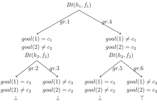
Example 3.2. Consider a DMM game item DM(l = 2, k = 3, n = 2). This item has 2 pins, 3 types of flowers, and 2 rows. Leth1(1) :=c1,h1(2) :=c2,f1 :=gr andh2(1) :=c3,

h2(2) := c2, f2 := gr. The default tree and least tree for this game item are the same, which is depicted in Figure 3.3. Number of steps are counted at each gr-edge, and for this game item the application steps for gr is 6, application steps foroo,rr and or are all 0.

Bt(h1, f1)

goal(1) =c1

goal(2)6=c2

Bt(h2, f2)

goal(1) =c3

goal(2)6=c2

⊥ gr.2

goal(1)6=c3

goal(2) =c2

⊥ gr.3

gr.1

goal(1)6=c1

goal(2) =c2

Bt(h2, f2)

goal(1) =c3

goal(2)6=c2

⊥ gr.5

goal(1)6=c3

goal(2) =c2

> gr.6

[image:22.595.170.424.227.395.2]

gr.4

Figure 3.3: Tableaux tree for Example3.2

Regression results The application steps are treated as the size of the decision tree in

Gierasimczuk et al. (2013), and are used as the complexity measurement of the tableaux model of DMM. The application steps of a DMM game item is a tuple of four, and each element in the tuple represents the application steps for a feedback type. Gierasimczuk et al. (2013) tested how well application steps predicted item ratings on 100 2-pin DMM game items, and the results showed high correlation. A basic regression model that only considered basic game features such as number of flower types, number of clues, and whether all flowers were used in the clues, could only explain 34%4 of the variance. However, the regression model that incorporated application steps based on the default decision tree could explain 70% of the variance, and the regression model that incorporated application steps based on the least decision tree could explain 75% of the variance. This showed that application steps computed by the analytical tableaux model can predict item ratings very well, and the size of the decision trees is a possible explanation for the cognitive difficulty of 2-pin DMM game items.

4_{Results in}_{Gierasimczuk et al.}₍₂₀₁₃_{) were generated based on the 2013 dataset of DMM. In Chapter}

(23)

3.3 Caveats

Even though the analytical tableaux model is able to correctly predict the the Elo ratings of game items, some of the assumptions and limitations of this model limit its ability to adequately explain the cognitive difficulty of DMM game items.

[image:23.595.317.502.331.451.2]

Order-dependency The procedure for building a decision tree in the analytical tableaux model is order dependent. According to the rules of analytical tableaux, a decision tree has to be unfolded step by step. In the case of DMM, a step is a Boolean formula that represents a clue. Therefore, in a DMM game, the analytical tableaux model depicts an agent as reasoning about clues one by one. Hence, the analytical tableaux model makes strong assumptions on the order in which players reason about clues when working on a game item.

Figure 3.4: Game item with four all gr feedbacks

However, researchers have observed that in reality players also reason across clues. When children saw game items whose feedbacks are all gr and the same flower appeared at the same position in the clues, they chose that flower and put it in the same position as in the clues for their answer. Self-reports of children supported that some children did recognize this pat-tern of all gr feedbacks. By applying some logic reasoning, clues that all contain gr

feedbacks form a logical shortcut for solving that game item. Researchers also speculated that children are even able to use this pattern in game items with more pins. Figure 3.4

gives an example of an all gr game item. In these kinds of cases the analytical tableaux model provides an incorrect prediction by stating this item is very difficult because it generates a huge decision tree that branches four times, whereas this item is, in fact, easy because children can recognize the all gr pattern across clues.

(24)

3.3. Caveats

the cognitive difficulty of a 2-pin DMM game item.

Even though the tableaux model implicitly assumes that decision trees are how children solve a game item, in practice uncovering the actual reasoning procedure that children use is quite difficult. Instead of reasoning by cases, children may also think in different ways, such as deliberating over possible answers and eliminating impossible conjectures. Therefore, it is too strong to assume that decision trees generated by tableaux is the cognitive process for solving that game.

(25)

Dynamic Epistemic Logic Model

We saw an analytical tableaux model for 2-pin DMM game items. This model was able to correctly predict 75% of the ratings of game items, but is also challenged for claiming to represent the cognitive process of solving DMM games without accounting for observed reasoning patterns. Since children may solve DMM games using processes other than reasoning by cases, can some other model capture those processes? Can we cross-check the reliability of the tableaux model by another model based on a different formalization?

The answer to each of these questions is yes. In this chapter we explore a Dynamic Epistemic Logic (DEL) model of 2-pin DMM game items. The DEL model of DMM game items does not include an assumption of reasoning by cases, and it allows agents other ways of solving a 2-pin DMM game item such as by deliberating over possible options. The DEL model can represent both order-dependent and order-independent ways of solving a game item, and provides a nice representation of cross clue logical shortcuts like the allgr

feedback pattern discussed earlier. In addition to these benefits, the DEL model of DMM game items is at least as general as the tableaux model because each tableaux decision tree for a DMM game item can be translated into a DEL model of the same game item.

In this chapter, we present the DEL formalization of DMM game items and the DEL way of solving a 2-pin DMM game item. We present two variants of the DEL model. One is order-dependent, and the other order-independent. We discuss and define complexity measurements of the DEL models, and show how to translate a tableaux decision tree into a DEL model, and end this chapter by presenting the DEL account for cross clue logical shortcuts.

4.1 DEL Preliminaries

(26)

4.1. DEL Preliminaries

As a unifying framework of both epistemics and dynamics, DEL extends basic epis-temic logic with event models and product updates, and thus becomes a powerful frame-work that can model sophisticated belief revision, information flow in social interactions, and many other phenomena (Baltag et al.,1998;van Ditmarsch et al.,2007;van Benthem et al., 2006). The basic language of DEL is the same as standard epistemic logic.

Definition 4.1 (Language). The language of of single-agent epistemic logicLX is gener-ated by:

ϕ ::= p | ¬ϕ | ϕ∧ϕ | Bϕ

where p ∈ Φ and Φ is a countable set of atomic sentences. ∨ and → are defined in the standard way. Bϕreads like “believe ϕ”.5

In DEL, the epistemic states of agents are represented by epistemic models.

Definition 4.2 (Epistemic model). An epistemic model ofLX is a tupleS =hS,|| · ||, s∗i where S is a set of possible worlds that are epistemically possible, || · || : Φ 7→ P(S) is a valuation assigning to each p∈Φ a set||p||S of worlds, and s∗ is the actual world.

This model provides sphere semantics forLX, which differs from the standard Kripke semantics for epistemic models, by not having indistinguishablity relations. Therefore, possible worlds are not connected in this epistemic model; instead, they are evaluated as sets. The sphere models are less general than Kripke models for LX, but is enough for modeling DMM game items and solutions. For any world w in a model S and any sentence ϕ, we writew|=_S ϕif ϕis true in the world w. When the modelS is fixed, we omit the subscript and simply write w|=ϕ. For atomic sentences,w|=ϕis given by the valuation:

w|=p iff w∈ ||p||

The semantics for other propositional formulas is given by the usual truth clauses:

w|=¬ϕ iff w6|=ϕ

w|=ϕ∧ψ iff w|=ϕand w|=ψ

The semantics for the belief operator B is given by:

w|=Bϕ iff t|=ϕfor all t∈S

Definition 4.3 (Event model). An event model is E = {E, pre},6 _where _e _∈ _E _{is an}

action, and pre is a sentence in LX that describes the precondition ofE.

5_{In the standard epistemic logic, there is another modal operator} _Kϕ_{that reads “know}_ϕ_{”. For the}

scope of this thesis, the belief operatorBis enough for our modeling, and therefore we omit this operator.

6_{We omit the indistinguishablity relation (}₋A_→_{) here because: (a) this is a single-agent model, so we do}

(27)

Given epistemic models and event models defined above, agents update their beliefs according to the product update protocol:

Definition 4.4 (Product update). The product update model is defined as S⊗E = (S⊗E,|| · ||)

where {(s, e)∈S⊗E |s |=pree} and ||p||_S⊗E :=s ∈ ||p||S.

4.2 Model of Game Items

In this section, we present the DEL formalization of DMM game items and how to solve a DMM game item via product update in DEL. This section divides into two subsections. The first subsection formalizes static information of a DMM game item shown on the screen. The second shows how to use DEL techniques to model the process of finding the secret flower code.

4.2.1 Formalizing Game Items

We formalize the static information shown on the screen for a DMM game item in this subsection, and we call this formalization the DMM game model. The DMM game model is introduced in three steps, first we show the mapping of flower pegs and feedback pegs to propositional letter, then we introduce sentences that represent flower sequences and clues, and lastly we define a feedback function that encodes how feedback pegs are given with respect to the secret sequence and a flower sequence.

Atomic sentences

The set of atomic sentences Φ consists of propositional letters for flower pegs and feedback pegs, as well as indexed propositional letters for flower pegs in flower sequences. We assign propositional letters as follows: p, q, . . .to lower pegs,gto green feedback pegs,oto orange feedback pegs, and r to red feedback pegs. For flower pegs in a flower sequence, index ·i

denotes the position of each flower in the sequence.

(28)

4.2. Model of Game Items

We can concatenate n propositional letters for feedback pegs to form a feedback se-quenceσn_{. For example, a 2-pin DMM game items has four possible feedbacks: green-red,}

red-red, orange-orange and orange-red. Hence, the four possible feedback sequences σ2 are gr, rr, oo, and or. When n = 1, the three possible feedback sequences σ1 _{are the} three propositional letters for feedback pegs, namely, g, r, and o. We include feedback sequences σn_{, n}_≥_{1 in the set of atomic sentences Φ as well.}

Altogether, the set of propositional letters Φ consists of flower pegs p, q, . . ., indexed flower pegs pi, qj, . . ., and feedback sequences σn, n≥1.

DMM game model

For every DMM game item, each clue consists of a conjecture and a corresponding feed-back. The conjecture consists of n flower pegs and the feedback consists of n feedback pegs. Formally, we define a clue as follows.

Definition 4.5 (Clue). A clue L=

n

V

i=1

xi∧σn, x, xi, σn∈Φ.

In Definition4.5, thexofxi ranges over propositional letters for flowersp, q, . . ., and i

is the position of the flower in the clue. The feedback sequence σn _{in the clue has length} n, which equals the number of indexed flower pegs. Note thatσn _{is a propositional letter}

in our language. We call the conjunction of all the xis in a clue L aflower configuration,

and denote it with C. A clue is a conjunction of a flower configuration C =

n

V

i=1

xi and a

feedback sequence σn_{. For every clue, each position in the flower configuration shall be}

filled with exactly one flower. In other words, for all 1 ≤i ≤ n, there exists exactly one

xj such that xi = xj. If pi, qj are in the same clue and i = j, then p = q; but not the

converse.

Example 4.2. Figure 2.2 shows 2 clues of a game item. In the first row clue L1 =

b1∧b2∧gr, and in the second row clue L2 =b1∧d2∧oo.

The secret code, orgoal(the only correct answer of the game), is a flower configuration that is hidden from agents in the game.

We now define the game model for DMM game items.

Definition 4.6 (DMM game model). A DMM game modelG is a tuple hFG,LG, goalGi

where FG is a set of indexed flower pegs that are available for players to choose from, LG

is the set of clues, and goalG is the secret code.

(29)

Example 4.3. For example, consider again the game item in Figure 2.2. Let G be the DMM game model of this game item, F ={a1, a2, b1, b2, c1, c2, d1, d2}, and L ={L1, L2}. As in Example 4.2, clue L1 =b1∧b2∧gr, and clue L2 =b1∧d2 ∧oo. Note thatgoal is not on the screen.

Feedback function

We want to not only describe DMM game items in DEL, but also encode the information needed for an agent to solve those game items. At the top-right corner of the screen shot in Figure 2.2, 3 rules state the relation between feedback pegs, conjectures, and the secret code. Accordingly, we define the following function to represent these pieces of information.

Definition 4.7. Given a DMM game model G = hF,L, goali, a clue L ∈ L and all the

pi that appear in L:

fgoal(pi) =

            

g if there is a qj in goal such that p=q and i=j;

o there is a qj in goal such that p=q and i6=k

and there is no rk inL such thatq =r and j =k;

r otherwise.

LetC be the flower configuration in clue L, with a slight abuse of notation, we write

fgoal(C) =σn as the result of concatenating fgoal(pi) for allpi that appears inC.

There-fore, a clue L=C∧σn =C∧fgoal(C).

Example 4.4. Take game model G in Example 4.3, it is the case that fgoal(C1) =

fgoal(b1∧b2) =gr and fgoal(C2) =fgoal(b1∧d2) = oo.

The feedback function specifies the relation between a flower configuration C in clue

Land thegoalconfiguration. It encodes information for solving a DMM game item. This definition can be relaxed to any flower configuration instead of just goal, which we will use later.

4.2.2 Solving Game Items

Now that we have formalized DMM game items into DMM game models, we can build DEL models for each game model to analyze the procedure of solving the game.

(30)

Taking the framework of DEL, we get the syntax and semantics for epistemic model, event model and product update for free. What remains to be specified are the valuation function and preconditions. Let us examine them one by one.

Valuation function

In an epistemic modelS={S,||·||, s∗}, a possible worlds∈Ssuch thats|=ϕrepresents a possibility that ϕis true at s. As for modeling DMM game items, we want each possible world s to represent a possible flower configuration. In other words, for each possible flower configuration C, we want one possible world s∈S such that s|=C.

Recall that a flower configuration C is a conjunction of indexed flower pegs,

n

V

i=1

xi.

Hence, by the semantics of DEL, we want the valuation function || · || to map the set of indexed flower pegs FG to the power set of possible worlds P(S), i.e., || · ||:FG7→ P(S).

The actual world s∗ |= goal. Atomic sentences that are not in the set of indexed flower pegs are mapped to the empty set, i.e., || · ||: Φ\FG7→∅.

Before an agent reasons about any clue, every flower configuration is a possible answer for the game. We call the epistemic model before updating with any event models the initial epistemic model. Hence, the number of possible worlds in the initial epistemic model is the same as the number of all possible flower configurations.

Proposition 4.1. Let S = {S,|| · ||, s∗} be an initial epistemic model for n-pin DMM game model G, if |FG|=m·n, then |S|=mn.

Proof. This comes from basic combinatorial calculations. SinceGis an-pin game,|FG|= m·nmeans that there aremtypes of available flowers pegs. A flower sequence, represented by a flower configuration, has n spots, and each of the n spots can choose from m types of flower pegs. Hence, there are mn combinations.

Following from this proof, each possible world in an epistemic model of a DMM game item represents an unique flower configuration C. Formally, for any s, s0 ∈ S such that

s |=C, s0 |=C0, if C =C0, then s=s0. We writeCs to denote the flower configuration C

that is true at world s.

Precondition

(31)

To model this reasoning process, we define event modelsELto represent the action of

reasoning about a clue L∈ LG. Given a DMM game model G, we define an event model

EL={eL, pre}whereeLis the action of observing clueL∈ LG, andpreis the precondition

for clueLto be true. For 2-pin DMM game models, we define four preconditionsprewith respect to each feedback sequence. Consider any clue L=p1∧q2∧σ2, then

If σ2 =oo, preeL =q1∧p2

If σ2 =rr, preeL =¬p1∧ ¬p2∧ ¬q1∧ ¬q2

Ifσ2 =gr, preeL = (p1∧ ¬q2)∨(q2∧ ¬p1)

If σ2 =or, preeL = (p2∧ ¬p1∧ ¬q1)∨(q1∧ ¬p2∧ ¬q2).

7

The precondition for σ2 =oo says that clue L= p1∧q2∧oo is true at worlds where the position of the two flower pegs in L are switched. The precondition for σ2 =rr says that L = p1 ∧q2 ∧rr is true at worlds where neither of the flower pegs in L appear in this world. The precondition for σ2 ₌ _gr _{says that} _L ₌ _p

1 ∧q2 ∧gr is true at worlds where one of the flower pegs in Lis at the right position and another flower peg does not appear. Finally, the precondition for σ2 ₌ _or _{says that clue} _L ₌ _p

1 ∧q2 ∧or is true at worlds where one of the flower pegs in L is the right flower at another position, and the other position holds neither flower pegs in L.

The product model S⊗E is defined as usual in DEL.

Now we need to show that the preconditions indeed capture the correct interpretation of each feedback, which we do by defining a notion of compatibility.

Definition 4.8 (Compatibility). A possible worlds is compatible with a clueL=C∧σn

if fCs₍_C_{) =} _σn_.

Recall that Cs is the flower configuration C that is true at world s. fCs(C) = σn

is an extension of the feedback function in Definition 4.7, and is defined by replacing

goal in Definition 4.7 with Cs. From the definition of the valuation, we know that each

possible worlds in an epistemic model holds a unique flower configurationCs. Therefore, fCs₍_C_{) =} _σn _{means that if} _s_{is the actual world, and} _C _{is the flower configuration in clue}

L=C∧σn_{, we get a feedback sequence} _σn0 _{such that}_σn0 ₌_σn_.

Proposition 4.2. Let S0 be an initial epistemic model for a game model G, EL =

{eL, pre}, where eL is the action of observing a clue L, then for S1 = S0 ⊗EL and S1 ∈S1, world s ∈S1 if and only if s is compatible with L.

7 _{According to the feedback function, the precondition for the} _or _{feedback to flower configuration}

p1∧q2can also bep2∧ ¬p1∧ ¬q1∧ ¬q2, and is equivalent to the precondition defined in the text, because

p1already indicates theq2cannot be the case, according to the condition of being a flower configuration

(32)

Proof. Without loss of generality, assume L=a1∧b2∧σ2. By the definitions of the DEL models in Section 4.1 and 4.2.2, S1 = {s|s ∈ S0 ⊗E} and S0 ⊗E = {(s, e)|s |= pre}. Note that (s, e) represents the possible worldswith label (s, e), hence,s∈S1 ⇔s|=pre. Hence, we need to show that for all s ∈S1:

• ⇒: if s∈S1, then fCs(a1∧b2) =σ2, and

• ⇐: if s6∈S1, then fCs(a1∧b2)6=σ2.

Let us check the four feedback sequencesoo, rr, gr, or one by one.

(i) σ2 =oo:

• ⇒: given anys ∈S1, by definition of pre,s|=a2∧b1. By definition of feedback sequence, fCs₍_a

1 ∧b2) =oo.

fCs₍_a

1)6=o, so that fCs(a1∧b2)6=oo. If s|=¬b1, thens 6|=b1, and fCs(b2)6=

o, fCs₍_a

1∧b2)6=oo. In all, if s6∈S1, then fCs(a1∧b2)6=oo. (ii) σ2 ₌_rr_:

• ⇒: given any s ∈ S1, by definition of pre, s |= ¬a1 ∧ ¬a2 ∧ ¬b1 ∧ ¬b2. By definition of feedback sequence, fCs₍_a

1∧b2) =rr.

g, fCs₍_a

1∧b2) 6=rr. Similarly for s |= a2, s |= b1 or s |= b2. In all, if s 6∈ S, then fCs₍_a

1∧b2)6=rr. (iii) σ2 ₌_gr_:

• ⇒: given any s ∈S1, by definition of pre, s|= (a1∧ ¬b2)∨(b2∧ ¬a1). Hence,

fCs₍_a

1) = g. By s 6|= b2, fCs(b2) = r. Hence, fCs(a1 ∧b2) = gr. Similarly for

s |=b2 ∧ ¬a1, we have fCs(b2) = g, fCs(a1) = r and fCs(a1∧b2) = gr. In all,

fCs₍_a

1∧b2) = gr.

• ⇐: given any s6∈ S1, by definition of pre, s 6|= (a1 ∧ ¬b2)∨(b2∧ ¬a1), hence,

s |= (¬a1 ∨ b2)∧ (¬b2 ∨a1). Suppose that s |= ¬a1, then s |= ¬b2, then

fCs₍_a

1)6=g andfCs(b2)6=g, thereforefCs(a1∧b2)=6 gr. Suppose thats |=b2, then s|=a1. Hence,fCs(a1) =g, fCs(b2) =g, therefore fCs(a1∧b2) =gg and

fCs₍_a

(33)

(iv) σ2 ₌_or_:

• ⇒: given anys∈S1, by definition ofpre,s|= (b1∧¬a2∧¬b2)∨(a2∧¬a1∧¬b1). Hence,s |=b1∧¬a2∧¬b2 ors|=a2∧¬a1∧¬b1. Suppose thats|=b1∧¬a2∧¬b2, by Definition 4.7, fCs₍_a

1) = r and fCs(b2) = o. Hence, fCs(a1 ∧b2) = or. Similarly for s|=a2∧ ¬a1∧ ¬b1. In all, fCs(a1∧b2) =or.

• ⇐: given any s6∈S1, by definition of pre,s|= (¬b1∨a2∨b2)∧(¬a2∨a1∨b1). Hence, s |= ¬b1∨a2 ∨b2 and s |= ¬a2 ∨a1∨b1. Suppose that s |= b1, then

s |= a2 ∨ b2. If s |= a2, then Cs = b1 ∧a2 and fCs(a1 ∧b2) = oo 6= or. If

s |= b2, then Cs = b1∧b2 and fCs(a1 ∧b2) = gr =6 or. Hence, if s |= b1 then

fCs₍_a

1∧b2)6=or.

Suppose thats |=¬b1, then s|=¬a2∨a1. Ifa |=¬a2, thens |=¬b1∧ ¬a2, and

fCs₍_a

1∧b2)6= or because there cannot be any o feedback for either flower. If

s |=a1, thenfCs(a1) =g and fCs(a1∧b2)6=or. In all,fCs(a1∧b2)6=or.

Therefore, in all, for any L=C∧σ2 and S1 =S0⊗E,

s ∈S1 ⇔fCs(C) = σ2.

Because of Proposition 4.2 and uniqueness of goalin the game setting, it follows that after updating with all clues, the DEL model converges to goal.

Theorem 4.1. For any 2-pin DMM game model G = (FG,LG, goal) where LG =

{L1, . . . , Ln}, let Ei = {ei, pre} where action ei is observing clue Li ∈ LG, then for

Sn=S0⊗E1⊗. . .En, |Sn|= 1.

Proof. By Proposition 4.2, it is always the case that the actual world s∗ ∈ Sn. Hence,

|Sn| ≥1. By uniqueness of goal, for all s ∈ |Sn| such that s is compatible with all clues

in LG, s=s∗. Hence, |Sn|= 1.

4.3 Sequential Update

(34)

4.3. Sequential Update

4.3.1 Illustration

Reasoning about clues one by one generates a sequence of epistemic models that shrink in size until only one possible world remains.

Example 4.5. Consider the game model G in Example 4.3, where the initial epistemic model is S0 = {S0,|| · ||, s∗}, and |S0|= 42 = 16. There are 16 possible flower configura-tions, each true at a unique possible world si ∈S0:

s1 |=a1∧a2, s2 |=a1∧b2, s3 |=a1∧c2, s4 |=a1∧d2,

s5 |=b1∧a2, s6 |=b1∧b2, s7 |=b1∧c2, s8 |=b1∧d2,

s9 |=c1∧a2, s10|=c1 ∧b2, s11|=c1∧c2, s12|=c1∧d2,

s13 |=d1 ∧a2, s14|=d1∧b2, s15|=d1∧c2, s16|=d1∧d2.

Let the following event models encode the two clues in the game model:

EL1 ={eL1, preL1}, sinceL1 =b1∧b2∧gr, preL1 = (b1∧ ¬b2)∨(b2∧ ¬b1), and

EL2 ={eL2, preL2}, sinceL2 =b1∧d2∧oo,preL2 =d1∧b2.

If the agent first reasons about clue L1, then the updated epistemic model is S1 = S0⊗EL1, S1 ={s2, s5, s7, s8, s10, s14}.

And reasoning about clue L2 results in the second updated epistemic model S2 = S1⊗EL2, S2 ={s14}.

Since|S2|= 1, and s∗ =s14, the goal is d1∧b2.

In Example4.5, the initial epistemic modelS0 has 16 possible worlds, and after updat-ing with clueL1,S1 has 6 possible worlds. Updating with clueL2 results inS2 where only the actually world is left. S0, S1 and S2 form a sequence of updated epistemic models, which we illustrate in Figure 4.1.

s1, s2, s3, s4

s5, s6, s7, s8

s9, s10, s11, s12

s13, s14, s15, s16

S0

s2, s5, s7

s8, s10, s14

S1

s14

S2

[image:34.595.169.424.538.612.2]

L1 L2

Figure 4.1: Illustration of the update sequence for Example4.5

We call such a sequence of updated epistemic models an “update sequence”. Formally,

Definition 4.9 (Update sequence). Let G be a (2-pin) DMM game model, S0 be the initial epistemic model, and E1, . . . ,En be event models for clues L1, . . . , Ln ∈ L, then

S1 =S0⊗E1,S2 =S1⊗E2, . . . ,Sn =Sn−1⊗En. An update sequence of this game model

(35)

As stated in Theorem 4.1, the update sequence of any DMM game model will end with the epistemic model of size 1, and for any epistemic models S, S0 in the same update sequence, if S is before S0, then |S| ≥ |S0|.

4.3.2 Complexity Measurements

We now define several criteria to measure the complexity of an update sequence generated by the DEL model of a DMM game model. We measure the complexity of an update sequence from the perspective of the number of possible worlds and the rate of convergence of the epistemic models respectively.

Size of epistemic models

One natural proposal is to take the sum of the sizes of all epistemic models in an update sequence. The size of an epistemic model reflects how many possibilities could serve as the correct answer, and hypothetically the more possibilities, the more difficult of this game item. Therefore, if a game item generates an update sequence in which each epistemic model contains many possible worlds, then this game is perceived to be more difficult. Formally,

Definition 4.10 (Measurement SUM0). The SUM0 complexity of an update sequence

Q=hS0, . . . , Sni is defined as

SUM0 :=

n

X

i=0

|Si|

We illustrate this measurement with the following example.

Example 4.6. Consider the following two game items.

(1) Game item 125966(Rating: -15.77):

G1 ={F1,L1, goal1},F1 ={a1, a2, b1, b2, c1, c2, d1, d2, e1, e2},|F1|= 5·2 = 10,

L1 ={L11, L21}, L11 =a1∧b2∧rr, and L21 =c1∧d2∧rr.

(2) Game item 125780(Rating: -30.15):

G2 ={F2,L2, goal2},F2 ={a1, a2, b1, b2, c1, c2}, |F2|= 3·2 = 6,

L2 ={L21, L22}, L21 =a1∧a2∧gr, and L22 =b1∧b2∧rr.

The sizes of the epistemic models in the update sequence forG1 are h25,9,1i, and for

(36)

4.3. Sequential Update

The Elo rating for G1 is -15.77 and the rating for G2 is -30.15, which means that empirically G1 is harder than G2. The SUM0 measurement for these two game items reflects this fact, with G1 of complexity measurement 35 and G2 of 14.

However, measurement SUM0 may overate the influence of the initial model, which we demonstrate in the next example.

Example 4.7. Consider game items (3) and (4), which have different sizes of initial epistemic models and therefore very different SUM0measurements. However, their ratings are very similar to each other.

(3) Game item 125831(Rating: -20.84):

G3 ={F3,L3, goal3},F3 ={a1, a2, b1, b2, c1, c2, d1, d2},|F3|= 4·2 = 8,

L3 ={L31, L23}, L31 =a1∧b2∧rr, L31 =c1∧d2∧oo.

(4) Game item 125563(Rating: -22.66):

G4 ={F4,L4, goal4},F4 ={a1, a2, b1, b2, c1, c2}, |F4|= 3·2 = 6,

L4 ={L41, L24}, L41 =a1∧a2∧gr, L41 =b1∧c2∧rr.

The sizes of epistemic models in DEL structure for G3 is h16,4,1i, and the sizes of epistemic models in the DEL structure for G4 is h9,4,1i.

According to Definition4.10, SUM0(G3) = 16+4+1 = 21 and SUM0(G4) = 9+4+1 = 14. However, the Elo rating of these two game items are very close to each other (-20.84 and -22.66). We therefore propose another measurement SUM1 that excludes the size of the initial epistemic models because the initial epistemic model simply contains all possibilities, which does not directly relate to how to solve the game. Formally,

Definition 4.11(SUM1). The SUM1 complexity of an update sequenceQ=hS0, . . . , Sni

is defined as

SUM1 :=

n

X

i=1

|Si|

This SUM1 measurement counts the number of possible worlds in an update sequence without counting the initial epistemic state, which avoids the situation illustrated in Example4.7. According to this new measurement, the SUM1measurement for the update sequence of game modelG3is 5, which equals the SUM1measurement for DEL structure of game model G4. This fits better with the Elo ratings for both items. We test whether the SUM1 measurement captures the empirical difficulty better than the SUM0 measurement in the next section.

(37)

Definition 4.12 (SV). The SV complexity of an update sequence Q = hS0, . . . , Sni is

defined as

SV := SUM0(Q)

n

Here, “V” stands for “average”, indicating that the SV measurement considers the average number of possible worlds per update. The higher the SV measurement, the more difficult a game item is.

Convergence rate

Another measurement of the complexity of DEL update sequences is the rate of conver-gence. If from Sk−1 to Sk, a clue Lk eliminates more states, then the faster this game

item converges togoal. Our assumption is the more possible worlds a clue eliminates, the more difficult it is for a player to reason about this clue.

Definition 4.13 (CR). The CR complexity of an update sequence Q = hS0, . . . , Sni is

defined as

CR :=

n

X

i=1

|Si−1|

|Si|

The CR measurement takes the sum of the convergence rate of an update sequence. The more states that get eliminated, the more reasoning is required for this step, and therefore we expect a higher rating. When increasing the number of states Si eliminates

from Si−1, |S_|_Si−1|

i| increases, resulting in a larger value that indicates a higher cognitive

difficulty of this game item.

Consider the four game models in Example 4.6 and Example 4.7, the CR complexity for each DEL structure of those game models are as follows:

CR(Q1) = 25

9 + 9

1 ≈11.78, CR(Q2) =

9 4+

4

1 ≈6.25, CR(Q3) =

16 4 +

4

1 ≈8, and CR(Q4) =

9 4+

4

1 ≈6.25.

(38)

4.4. Intersecting Update

measurement captures the fact the G1 is more difficult than the rest, and thatG3 is more difficult than G2, but not G4 is more difficult than G2 and G3, and that G2 is the least difficult.

4.4 Intersecting Update

As shown earlier, an update sequence is order-dependent. That is to say, the order of which clue to process decides the update sequence, and consequently influences the value of the complexity measurements of that game item. However, experiments that track eye movements reveal that people do not always follow a specific order in reasoning over clues (Truescu, 2016). Therefore, since assuming the order of clues to update in a DEL update is too strong, and we want to relax or drop this constraint on our DEL model.

Fortunately, updating clues one after one is not the only way to solve a DMM game item in the language of DEL. In fact, an agent can update the initial epistemic model using all the clues at the same time, and then take the intersection of such updates. According to the DEL formalization, this procedure always leads to goal as well.

Proposition 4.3. For a 2-pin DMM game model G, let S be an epistemic model,EL be

an event model for clue L∈ LG, and EL0 an event model for clue L0 ∈ L_G, then:

S⊗EL⊗EL0 =S⊗E_L0 ⊗E_L.

Proof. LetA=S⊗EL⊗EL0, andB =S⊗E_L0⊗E_L. Letϕ=WCsfor all s∈S, then for

all s ∈ S, s|= ϕ. By definition of product update, for all a ∈ A, a|= ϕ∧preeL∧preeL0,

and for all b ∈ B, b|= ϕ∧pree_L0 ∧preeL. Since all the preconditions pre do not contain

any modal operator, but are just propositional logic formulas, whetherpreis true in some world s depends only on the valuation ats, and not at any other world. By propositional logic, A=B.

Proposition4.3 shows that the order of an update does not effect the updated model. This proposition can be written in a different way:

Theorem 4.2. For a 2-pin DMM game model G, let S0 be the initial epistemic model and EL1, . . .ELn be event models for clue L, . . . , Ln:

S0 ⊗EL1. . .⊗ELn = n

\

k=1

S0⊗ELk

(39)

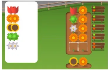
Figure 4.2: Screenshot of a 2-pin DMM game item

4.4.1 Illustration

Now we show by way of an example that we can find goal for a game item by updating each clue with the initial epistemic model and then taking the intersection of them.

Example 4.8. Consider the game item in Figure 4.2, which has game model G =

hF,L, goali, where F = {a1, a2, b1, b2, c1, c2}, L = {L1L2}, L1 = b1 ∧ b2 ∧ gr, and

L2 = c1 ∧ b2 ∧ gr. The initial epistemic model S0 = {S0,|| · ||, s∗},|S0| = 32 = 9. There are 9 possible flower configurations, each true at a possible world si ∈S0:

s1 |=a1∧a2, s2 |=a1∧b2, s3 |=a1∧c2,

s4 |=b1∧a2, s5 |=b1∧b2, s6 |=b1∧c2,

s7 |=c1∧a2, s8 |=c1 ∧b2, s9 |=c1∧c2.

Let event models encode the two clues in the game model as follows: EL1 ={eL1, preL1}, sinceL1 =b1∧b2∧gr, preL1 = (b1∧ ¬b2)∨(b2∧ ¬b1).

EL2 ={eL2, preL2}, sinceL2 =c1∧b2∧gr,preL2 = (c1∧ ¬b2)∨(b2∧ ¬c1).

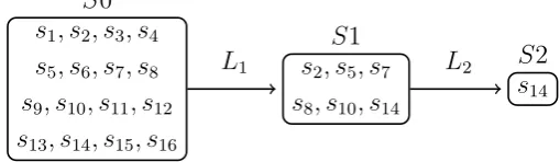
Updating the initial epistemic model with clue L1 results in the updated epistemic model S1 =S0⊗EL1, S1 ={s2, s4, s6, s8}.

And updating the initial epistemic model with clueL2results in the updated epistemic model S2 =S0⊗EL2, S2 ={s2, s5, s7, s9}.

IntersectingS1 andS2 leads to the actual world,S1∩S2 ={s2}, s∗ =s2, goal=a1∧b2.

Figure 4.3 shows the update sequence for Example 4.8. In this case, the initial epis-temic model is updated with each clue individually, and then the intersection of all the updated models is taken, which leads to the secret sequence goal.

[image:39.595.190.410.108.218.2]

(40)

4.4. Intersecting Update

s1, s2, s3,

s4, s5, s6,

s7, s8, s9.

S0

s2, s4,

s6, s8.

S1

s2, s5,

s7, s9.

S2

[image:40.595.195.401.99.245.2]

L1 L2

Figure 4.3: Illustration of the update sequence for Example4.8

Definition 4.14 (Unordered update sequence). For any event modelsEi ∈ {E1, . . . ,En},

an unordered update sequence is a set U =hS0, . . . , Sni where Sn ∈ Sn such that Sn =

S0⊗En.

4.4.2 Complexity Measurements

There are several ways of measuring the complexity of an unordered update sequence. On the one hand, the measurements we defined for update sequence can be applied to unordered update sequence with minor modifications. On the other hand, we can also measure complexity of an unordered update sequence with respect to different feedback types.

Complexity measurements SUM0, SUM1 and SV can be applied on unordered update sequences. The only change is that whereas Si in an ordered update sequence refers to

the i-the iteration, in an unordered update sequence it simply refers to an update of the initial epistemic model, but the calculations are the same. The complexity measurement CR is modified as follows:

CR’ :=

n

X

i=1

|Si|

|S0|

,

because for each Si, i > 0 is the result of updating clue Li against the initial epistemic

model, hence we should take the ratio of |Si| against|S0| accordingly.

(41)

0. Besides computing the number of possible worlds that survive an elimination, we can also compute the ratio of the number of worlds that survive to the number of worlds in the initial epistemic model, as an echo to the concern about convergence rate discussed in earlier sections. Listing 4.1 shows the R code of the algorithm that we use in computing these measurements for the unordered update sequence for each 2-pin DMM game item.

Listing 4.1: Rcode for measurements over unordered update sequence

f o r ( i i n 1 : nrow( 2 p i n DMM) ){ i f ( c l u e [ i ] == oo ){

oo <− oo + x

} e l s e i f ( c l u e [ i ] == r r ){

r r <− r r + x

} e l s e i f ( c l u e [ i ] == g r ){

g r <− g r + x

} e l s e i f ( c l u e [ i ] == or){ or <− or + x

} }

We define two complexity measurements using the this algorithm. One is the DELs measurement, which considers the number of possible worlds that get selected per feedback type, and the other is the DELr measurement, which considers the ratio of the selected possible worlds to the initial epistemic model per feedback type. We first compute a value

x for each clue, and then average x with respect to feedback types. For measurement DELs, x is the size of epistemic model Si after updating the initial epistemic model with

event model Ei that contains clue Li. For measurement DELr,x is calculated as |S i| /

|S 0| for a given DEL structure. All feedbacksoo,rr,gr,or are initialized as 0. Hence, if a feedback σ does not appear in a game model, the evaluation for feedbackσ remains 0. Both the DELs and DELr measurements are averaged by the number of appearance of that feedback.

Consider the game item in Example 4.5. The size of the initial epistemic model is 16. One clue has a gr feedback, which leads to an updated epistemic model of 6 possible worlds. Another clue has a oo feedback, which leads to an updated epistemic model of only 1 possible world. The unordered update sequence for this game item is h16,6,1i, with 6 for gr and 1 for oo. Hence, the DELs measurement for this item is

hoo= 1, rr = 0, gr = 6, or = 0i

And the DELr measurement for this item is

hoo= 1

16, rr = 0, gr = 6

16, or = 0i

(42)

4.5. Informativeness of feedbacks

[image:42.595.82.514.182.254.2]

last two measurements only apply to unordered update sequences and take feedback type into account. In the next chapter, we test these measurements with the empirical dataset of item ratings.

Table 4.1: Summary of complexity measurements

Complexity

Measurement SUM0 SUM1 SV CR DELs DELr

Definition

n

P

i=0

|Si| n

P

i=i

|Si| SUM_n 0 n

P

i=0 |Si−1|

|Si|

SUM0 per feedback type

CR per feedback type

4.5 Informativeness of feedbacks

Before testing our complexity measurements with empirical dataset, let us pause a bit in and take a closer look at how each clue eliminates possible worlds differently in the elimination process.

The number of possible worlds eliminated relates to the notion of informativeness. In information theory, informativeness of the occurrence of an event is defined by its entropy. The less likely the occurrence of the event is, the more information it contains. Entropy can also be viewed as the bits needed to encode the occurrence of the information. It was first studied byShannon (2001), and then developed into an important area of study. Measuring informativeness of information based on the probability distribution is used in many research areas. In particular, Fangzhou et al. (2015) used this measurement to simulate human reasoning of logic rules in syllogistic reasoning. In the DEL models of 2-pin DMM game items, a natural correspondence to informativeness of clues is the number of possible worlds eliminated by an update. Assume that an agent is currently at epistemic model S with |S|=m. From Section 4.2, for each s∈S, s|=Cs where Cs is a possible flower configuration that could be an answer of this game. Hence, the probability of each s being s∗

P(s=s∗) := 1

|S| (4.1)

When |S|= 1, P(s∗ =s∗) = 1, in accordance with Theorem 4.1.

Definition 4.15 (Elimination power of clues). LetE be an event model where eL is the

action of observing clue L, S0 is the initial epistemic model before updating withE, and S=S0⊗E, then the elimination power of clue Lis defined as

El(L) :=|S|