An Interpretation of Flare-Induced and Decayless Coronal-Loop Oscillations as Interference Patterns

promoting access to White Rose research papers

White Rose Research Online

[email protected]

Universities of Leeds, Sheffield and York

http://eprints.whiterose.ac.uk/

This is a copy of the final published version of a paper published in

The

Astrophysical Journal

.

This article is distributed under the terms of the American Astronomical Society,

who retain copyright over the article.

White Rose Research Online URL for this paper:

http://eprints.whiterose.ac.uk/79591

Published paper

The Astrophysical Journal, 784:103 (10pp), 2014 April 1 doi:10.1088/0004-637X/784/2/103

C

2014. The American Astronomical Society. All rights reserved. Printed in the U.S.A.

AN INTERPRETATION OF FLARE-INDUCED AND DECAYLESS CORONAL-LOOP

OSCILLATIONS AS INTERFERENCE PATTERNS

Bradley W. Hindman1and Rekha Jain2

1_{JILA and Department of Astrophysical and Planetary Sciences, University of Colorado, Boulder,}

CO 80309-0440, USA;[email protected]

2_{School of Mathematics & Statistics, University of Sheffield, Sheffield S3 7RH, UK}

Received 2013 December 5; accepted 2014 January 31; published 2014 March 11

ABSTRACT

We present an alternative model of coronal-loop oscillations, which considers that the waves are trapped in a two-dimensional waveguide formed by the entire arcade of field lines. This differs from the standard one-two-dimensional model which treats the waves as the resonant oscillations of just the visible bundle of field lines. Within the framework of our two-dimensional model, the two types of oscillations that have been observationally identified, flare-induced waves and “decayless” oscillations, can both be attributed to MHD fast waves. The two components of the signal differ only because of the duration and spatial extent of the source that creates them. The flare-induced waves are generated by strong localized sources of short duration, while the decayless background can be excited by a continuous, stochastic source. Further, the oscillatory signal arising from a localized, short-duration source can be interpreted as a pattern of interference fringes produced by waves that have traveled diverse routes of various pathlengths through the waveguide. The resulting amplitude of the fringes slowly decays in time with an inverse square root dependence. The details of the interference pattern depend on the shape of the arcade and the spatial variation of the Alfv´en speed. The rapid decay of this wave component, which has previously been attributed to physical damping mechanisms that remove energy from resonant oscillations, occurs as a natural consequence of the interference process without the need for local dissipation.

Key words: magnetohydrodynamics (MHD) – Sun: Corona – Sun: magnetic fields – Sun: oscillations – waves

Online-only material:color figures

1. INTRODUCTION

The detection of standing kink-wave oscillations on bright coronal loops by theTransition Region and Coronal Explorer

instrument (e.g., Aschwanden et al. 1999; Nakariakov et al.

1999) proffered the possibility first suggested by Roberts et al. (1984) that seismic techniques could be applied to magnetic structures in the corona. Given that the magnetic field of the corona remains resistant to measurement by spectroscopic means, coronal-loop seismology permits the direct probing of an otherwise inaccessible (yet paramount) property of the corona. Two observational details suggest that many of the observed motions are those arising from resonant standing waves with wavelengths corresponding to the fundamental mode. These observational details are that different segments of the loop are often observed to vacillate in phase with each other and the sinuous motion often lacks nodes, except perhaps at the loop footpoints (e.g., Aschwanden & Schrijver2011; Anfinogentov et al.2013). In some instances in addition to the fundamental mode with the lowest frequency, coexistent overtones (with interior nodes and a higher frequency) have been detected (Verwichte et al.2004; Van Doorsselaere et al.2007; De Moortel & Brady2007). The discovery of such overtones precipitated a tumult of theoretical activity with the goals of both explaining the observed dispersion and developing seismic methods that use the dispersion to surmise the field strength and mass density along the loop (see the review by Andries et al.2009).

The first oscillations to be detected were the response of loops within coronal arcades to the passage of transient disturbances launched from solar flares. It has been observed that such oscil-lations, once initiated, rapidly diminish over three to four wave periods (e.g., White & Verwichte2012). A variety of

theoret-ical studies have suggested possible damping mechanisms to explain the observed diminuation of the signal, with the most prominent being resonant absorption (e.g., Ruderman & Roberts

2002; Goossens et al.2002,2011) and phase mixing between distinct fibrils in a bundle, each with slightly different wave speeds (Ofman & Aschwanden2002). In all cases the diminu-ation of signal results from a physical loss of energy from the observed kink waves.

Recent observations (Nistic`o et al.2013; Anfinogentov et al.

2013) using the Atmospheric Imaging Assembly on theSolar Dynamics Observatoryhave revealed that in addition to these large-amplitude flare-induced oscillations there appears to be a continuous background of fluctuating power that oscillates at frequencies similar to the flare-induced waves, but with a lower amplitude that does not exhibit significant attenuation. These studies have posited that the background oscillations are excited by a continuous, and perhaps stochastic, driver whose energy input is balanced on the long term by physical damping. Thus, the two classes of oscillation are caused by waves with the same resonant nature, but excited by different sources, one ongoing and the other impulsive.

(a) (b)

Figure 1.Schematic diagram of a coronal arcade. Thex–yplane corresponds to the photosphere and the height above the photosphere is given byz. (a) Three-dimensional view of the thin sheet of magnetic field lines that define the arcade. The arcade lacks shear and is invariant along the axis of the arcade in they-direction. (b) Cross-sectional cut through the arcade at constantyshowing a thin annulus. The triad of unit vectors for the local Frenet coordinates are shown in red, with the tangent vectorˆs, the principal normalηˆ, and the binormalˆy. Each field line has a length ofLfrom photosphere to photosphere. For the sake of presentation, we assume that each field line forms a semicircle.

(A color version of this figure is available in the online journal.)

and that flares often cause the entire arcade to ring and throb. The second property is that many of the standing waves that have been observed possess a “horizontal” polarization such that the loop sways back and forth within the arcade (e.g., Verwichte et al. 2009). This implies that the motion of a loop impacts neighboring (and possibly invisible) field lines within the ar-cade and forces them to move. The individual bundles of field lines that form loops are therefore not isolated from the larger arcade structure in which they are embedded. Here we suggest that the arcade forms a two-dimensional waveguide and that the observed ringing is a superposition of waveguide modes that form in response to driving by flares and other sources. The waves are inherently two-dimensional modes that are trapped standing waves longitudinal to the field, while propagating up and down the axis of the arcade perpendicular to the field. We will find that such a model naturally leads to decaying signals without the need for a physical damping mechanism. The atten-uation of the sinusoidal signal observed at a given field line or loop is a fringe pattern resulting from the self interference of a wavefront as it expands away from a point source.

In Section2we derive a simple wave equation that describes MHD fast waves that propagate on a thin two-dimensional sheet of arching field lines. We define the geometry of the field and describe the boundary conditions that turn the arcade into a waveguide. In Section3 we derive the response of the waveguide to two types of sources, a continuous stochastic source and an impulsive source. Finally, in Section4we discuss the implications of our calculation and present our conclusions.

2. MHD FAST WAVES IN A WAVEGUIDE

We treat a coronal arcade as a thin magnetized sheet with each field line in the sheet piercing the photosphere at two locations. The locus of the footpoints for all of the field lines form two parallel lines in the photosphere. If we view the photosphere as a dense, immovable fluid, waves are trapped between the footpoints and the arcade acts as a two-dimensional waveguide for MHD fast waves that permits free propagation up and down its axis perpendicular to the field. We utilize a Cartesian coordinate system oriented such that thex–yplane corresponds to the photosphere and thezcoordinate is the height above the photosphere. Let the arcade be invariant in they-direction and

let it lack shear such that the field has no component in that direction,

B=Bx(x, z)xˆ +Bz(x, z)zˆ. (2.1)

Figure 1 provides a schematic diagram of the arcade and its geometry.

For simplicity, we will assume that the corona is magnetically dominated such that gravity and gas pressure can be ignored when compared to the magnetic forces. Furthermore, in order to build an illustrative example without unnecessary mathematical complication, we will ignore the curvature of the field lines within the wave equation and assume that the Alfv´en speed

VA within the sheet is uniform. With these assumptions, fast

MHD waves can be conveniently expressed using local Frenet coordinates. The triad of unit vectors that represents this local coordinate system are the tangent to the field line ˆs, the field line’s principal normalηˆ, and the binormal ˆy. The tangential coordinatesmeasures the pathlength along a field line starting from the photosphere, with the footpoints located ats=0 and

s = L, where the length of each field lineLis the same. The coordinateymarks distance along the axis of the waveguide and we assume that the arcade is long enough that we can ignore edge effects.

2.1. Equation for Driven Fast Waves

Since we are only considering magnetic forces, fast MHD waves lack motion parallel to the field lines and the transverse motion is irrotational. The fluid velocity,u, can be decomposed into two related components,

u=vˆy+wηˆ, (2.2)

∂v ∂η =

∂w

∂y, (2.3)

where v is the fluid velocity in the binormal direction andw

is the component in the normal direction. Further, driven fast waves satisfy the following simple equation,

∂2

∂t2 −V 2 A

∂2

∂y2 +

∂2

∂s2 +

∂2

∂η2

The Astrophysical Journal, 784:103 (10pp), 2014 April 1 Hindman & Jain

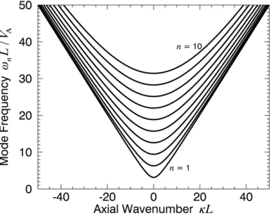
Figure 2.Eigenfrequencies,ω2n=(λn2+κ2)VA2, of the modes of the waveguide

as a function of the wavenumberκ parallel to the waveguide’s axis. Each curve corresponds to a different mode ordernlabelling the discretely allowed wavenumbersλn=nπ/Lin the direction parallel to the field. The gravest mode (n=1) has the lowest frequency, and each higher order has a correspondingly higher frequency.

where S(x, t) is a wave driver, the Alfv´en speedVAis given

byV_A2 =B2/4πρ, andρ is the mass density. In observational contexts, motions in the direction of the principal normal,w, are often referred to as “vertical” oscillations, whereas velocities

v in the binormal direction, along the axis of the arcade, are called “horizontal” oscillations. We will explore horizontal oscillations (w=0) by supposing that the driver only acts in the binormal direction and lacks variation across the arcade’s sheet, i.e., the driver is independent of the coordinateη. With these assumptions, only two-dimensional wave modes are excited and they obey the following equation:

∂2 ∂t2 −V

2 A

∂2 ∂y2 +

∂2 ∂s2

v=S(s, y, t). (2.5)

We make the arcade into a waveguide by imposing boundary conditions at the footpoints. Specifically, we apply the line tieing condition at the photosphere (i.e.,v =0 ats =0 ands =L). The resonant modes of this waveguide form a discrete spectrum in the tangentials-direction and a continuous spectrum in the transversey-direction down the axis of the waveguide,

vn(s, y, t;κ)=Un(s)eiκye−iωn(κ)t, (2.6)

Un(s)≡

2

L

1/2

sin(λns), (2.7)

for positive mode ordersn=1,2,3,4,· · ·. The allowed parallel wavenumbersλnand the eigenfrequencyωn(κ) are given by

λn=

nπ

L , (2.8)

ω2_n(κ)=λ_n2+κ2V_A2. (2.9) The wave is a standing wave in the direction parallel to the magnetic field, with discrete wavenumbersλn, and a propagating

wave in the ydirection with continuous wavenumber κ. The temporal frequencyωn(κ) depends on both wavenumbers and is

illustrated in Figure2. The parallel eigenfunctions,Un(s), have

been normalized such that they form an orthonormal set. Our general strategy for solving the driven Equation (2.5) is as follows: we will Fourier transform the equation in the

invariant y-direction, decompose the source and solution into the eigenfunctions of the waveguide, solve for the amplitude of each mode in spectral space, and then return to configuration space by inverting the transform. After Fourier transforming the driven wave equation and projecting onto the eigenmodes of the waveguide, we obtain

∂2

∂t2 +ω 2

n(κ)

ˆ

vn(κ, t)= ˆSn(κ, t), (2.10)

where

ˆ

Sn(κ, t)=

_∞

−∞ dy

L

0

ds S(s, y, t)Un(s)e−iκy, (2.11)

ˆ

vn(κ, t)=

_∞

−∞ dy

L

0

ds v(s, y, t)Un(s)e−iκy. (2.12)

In configuration space, the solution is obtained by inverting the transform and summing over eigenmodes,

v(s, y, t)= 1 2π

_∞

−∞ dy

∞

n₌1

ˆ

vn(κ, t)Un(s)eiκy. (2.13)

A similar equation holds for the reconstruction of the source from its spectral decomposition,

S(s, y, t)= 1 2π

_∞

−∞ dy

∞

n=1

ˆ

Sn(κ, t)Un(s)eiκy. (2.14)

3. TWO-COMPONENT SIGNAL

We posit that the wave signal seen at the observation loca-tion y is a superposition of the waves generated by a source with two components: a broad-band driver that generates a low-amplitude, resonant, background signal and an energetic impul-sive source that generates a large initial pulse with subsequent ringing,

S(s, y, t)=Sbg(s, y, t) +Simp(s)δ(t−t)δ(y−y). (3.15)

The first termSbgrepresents the continuous, broad-band driver,

which could be the incessant buffeting from ambient waves in the corona external to the waveguide, or perhaps the random movement of the footpoints of the arcade in the photosphere by convective motions. The second termSimp is the impulsive

source arising from a single short duration event such as a flare. Of course each source will independently produce a wave response,

v(s, y, t)=v_bg(s, y, t) +v_imp(s, y, t). (3.16)

3.1. Resonant Background Oscillations

The background velocity resulting from the broad-band component of the source can be expressed as a superposition of waveguide modes. The amplitude and phase of each mode can be obtained by taking the temporal Fourier transform of Equation (2.10), solving for the velocity in spectral space, and inverting the temporal transform through contour integration (see AppendixA),

vbg(s, y, t)=

1 2π

∞

n=1

_∞

−∞

dκ An(κ)Un(s)

In this equation, An(κ) is the mode amplitude of the mode

andθn(κ) is the phase of the source function in spectral space,

evaluated at the mode frequencies,

ˆ

S_n(bg)(κ, ω)=

_∞ −∞ dt _∞ −∞ dy L 0

ds S_bg(s, y, t)

×Un(s)e−i(κy−ωt), (3.18)

ˆ

S_n(bg)(κ, ωn)=Sˆ(bg)n (κ, ωn)eiθn(κ), (3.19)

An(κ)≡

Sˆ(bg)n (κ, ωn)

ωn(κ)

. (3.20)

The amplitude of the modeAn(κ) depends on the modulus of the

source function evaluated at the mode frequency. The factor of frequency appearing in the denominator of the mode amplitude causes a white source to excite modes such that they all have equal energy. Since the energy in each modeEnis proportional to both the square of the amplitudeAn(κ) and the square of the

frequencyωn(κ), an amplitude that is inversely proportional to

its frequency corresponds to an equipartition of kinetic energy. Even if the source function possesses wavenumber dependence, we still expect the waves with the lowest frequency to dominate the background signal as long as the source is not a rapidly increasing function of wavenumber.

The phase of the response depends on the phase θn of

the source function and the variation of this phase over all wavenumbers κ comprising the signal. Since the signal has contribution from a range of frequencies around a dominant frequency, we expect the interference between the different frequencies to cause beat patterns that will slowly and randomly rotate the apparent phase of the oscillation in time. Therefore, at a given position along the waveguide, we should expect the resonant background to be dominated by the gravest mode and produce a signal with the following form,

vbg ≈Abg sin(π s/L) sin[(π VA/L)t+φ(t)], (3.21)

where the phaseφ(t) slowly changes with time (| ˙φn| π VA/L)

due to the continual excitation by the source.

We will see that this expectation holds true by exploring in more detail two types of background sources. In Figure3(a) we show the source strength (red curve) for a source with a Gaussian dependence on wavenumber,

Sˆ(bg)_n (κ, ωn)= ˜S exp

−κ2

2Δ2

δn1. (3.22)

In this equation,S˜is an arbitrary constant andΔis the spectral width of the Gaussian. For simplicity we have assumed that the source only excites the fundamental mode n = 1. We model a stochastic source by imposing that the phase of the sourceθn(κ) is a random function with a uniform distribution

between 0 and 2π. Figure3(a) also shows the mode amplitude

An(κ) as the black curve. This type of source generates an

amplitude spectrum that is sharply peaked at zero wavenumber with little contribution from the wings. Thus we expect that the corresponding time-series (shown in Figure 3(b)) should be dominated by the frequency ω₁ = π V_A/L, with a phase that slowly wanders. This is indeed the case. This time-series was constructed by numerically evaluating the inverse spatial transform in Equation (3.17).

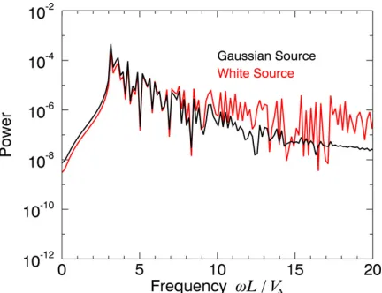
For the second source we choose a white source whose strength (by definition) is a constant function of wavenumber. The phase of the source function is once again chosen to be random. Figure 4 presents the amplitude spectrum and the resulting time series. Since the white source contains a broader range of wavenumbers, it generates a time-series with richer frequency response. In particular, we can clearly see from Figure4(b) that the time series possesses high-frequency jitter. The time-series generated by both sources are highly correlated with very similar low-frequency behavior. This is because the same realization of random phases was used to construct both sources. The equivalency of the set of phases also manifests in the temporal power spectra of the two time series (see Figure5). The fine structure in the two power spectra is similar because this structure arises from wave interference, which of course is determined by the relative phases (which were chosen to be identical).

3.2. Response to an Impulsive Source

The waves generated by the impulsive source are of course determined by the Green’s function. Therefore, consider a single point source of unit amplitude that occurs at time t and at location (s, y) = (s, y). We perform a detailed derivation of the Green’s function in AppendixB. The general procedure is to Fourier transform the wave equation in the axial directiony, decompose into waveguide modes, and solve for the temporal behavior. The solution is then reconstructed by summing over mode orders and inverting the spatial Fourier transform. After some manipulation of Equation (B9) this inverse transform is expressed as

G(s, s, y−y, t−t)= H(t−t

₎

2π ∞

n=1

_∞

−∞

dκ Un(s)Un(s)

×sin[ωn(κ) (t−t)]

ωn(κ)

eiκ(y−y),

(3.23)

whereHis the Heaviside step function. The inverse transform has an analytic solution (Weast et al.1989) involving zero-order Bessel functions of the first kind,J0,

G(s, s, y−y, t−t)= H(τ) 2V_A

∞

n=1

Un(s)Un(s)J0(λnVAT).

(3.24) We have written the solution compactly by defining the follow-ing delayed times:

τ ≡(t−t)−|y−y

_|

VA

, (3.25)

T ≡

(t−t)2−(y−y) 2

V2 A

. (3.26)

The Astrophysical Journal, 784:103 (10pp), 2014 April 1 Hindman & Jain

(a) (b)

Figure 3.Background oscillations described both in spectral space and as a function of time. The source strength| ˆS₁(bg)|is a Gaussian function of wavenumber, chosen to have unit amplitude (S˜ =1) and a width ofΔ=2π/L. (a) The source strength (red curve) and the resulting amplitude spectrumA1(κ)= | ˆS1(bg)|/ω1(κ) (black

curve) for the gravest mode (n=1) as a function of axial wavenumberκ. (b) The time series of the background oscillation as observed at the apex of the arcade,

s=L/2, and at an arbitrary position along the arcadey=yobs. The signal has a dominant frequencyω=nπ VA/L, with a phase that slowly wanders with time.

(A color version of this figure is available in the online journal.)

(a) (b)

Figure 4.Background oscillations described both in spectral space and as a function of time for a source that is white with a strength that is independent of wavenumber. (a) The mode amplitudeA1(κ) (black curve) of the background oscillations for the gravest mode (n=1) as a function of axial wavenumberκ. The source strength

is overlayed in red. Even though the source is white, the signal is dominated by the waves with the smallest axial wavenumbers and hence the waves with the lowest frequency (see Figure2). However, the wings of the amplitude distribution are more significant than they are for the Gaussian source. (b) The time series of the background oscillation as observed at the apex of the arcade,s=L/2, and at an arbitrary point along the arcadey =yobs. Since the wings are enhanced in the

amplitude distribution, the time series has more prominent high-frequency jitter. (A color version of this figure is available in the online journal.)

Figure 5.Temporal power spectra of the background oscillations illustrated in Figures3and4. The fine structure arises from the interference between waves and is, therefore, sensitive to the specific realization of wave phases. Here, for the sake of comparison, we have used the same realization for both types of source. The spectrum generated by the white source clearly has a greater contribution from high-frequency waves. Both spectra have a low-frequency cut-off that corresponds to the resonant mode frequencyω1 = π VA/Lappropriate for

propagation parallel to the field lines (i.e.,κ=0).

(A color version of this figure is available in the online journal.)

paths generates the oscillation pattern seen at any given point. This superposition is a combination of waves with different wavenumbersκ and hence directions of initial launch from the

source. This summation is represented by the integral in the inverse Fourier transform in Equation (3.23).

The response of the waveguide to the impulsive source appearing in Equation (3.15), Simp(s)δ(t −t)δ(y −y) is of

course the integral of the product of the Green’s function and the sourceSimp(s) over the point source’s locations,

vimp(s, y, t)=

H(τ) 2VA

∞

n=1

AnUn(s)J0(λnVAT) (3.27)

An≡

L

0

S_imp(s)Un(s)ds. (3.28)

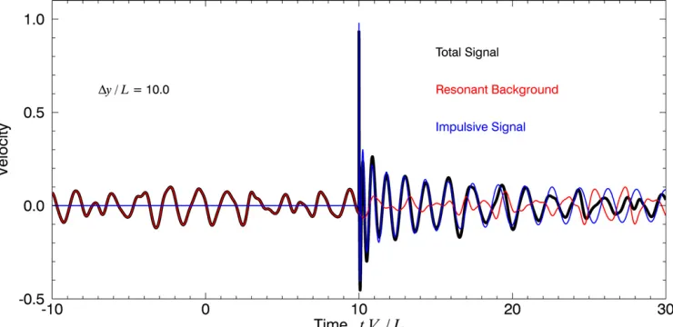
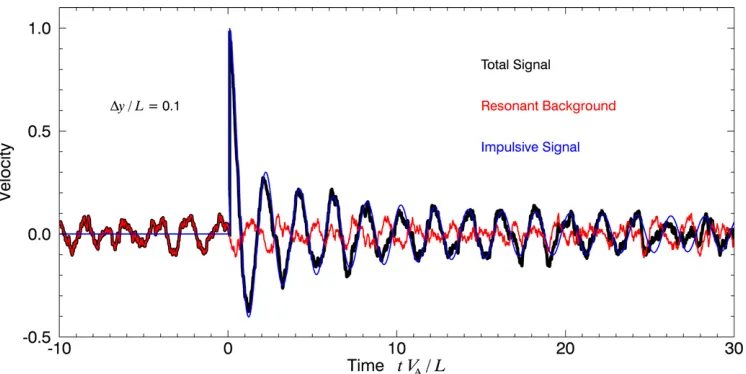
In Figures 6–8 we show this signal superimposed on the background oscillations. In all cases, the impulsive source occurs at timet = 0 and the waves are observed at the apex of the loops = L/2. Further, for simplicity we assume that only the gravest moden=1 is excited to significant amplitude (i.e.,|An| |A1|for n = 1). Figures6and8 correspond to

an impulsive event that occurs only a short distance away from the observation point,Δy =y−y=0.1L, while for Figure7

Figure 6.Wave signal as a function of time arising from both wave sources. The red curve is the background signal generated by a distributed stochastic source. The strength of the stochastic source is Gaussian in wavenumberκ(see Figure3(a)). The dominant frequency is the lowest frequency available, corresponding to those waves withκ=0 which propagate parallel to the magnetic field. The blue curve is the signal arising from a single impulsive event that occurred rather close to the observation point along the arcade,Δy=0.1L. The initial pulse corresponds to waves that have propagated straight down the waveguide, while the latter oscillations are an interference pattern arising from waves that have taken a variety of paths down the waveguide. The black curve shows the total wave signal. We have chosen the relative size of the impulsive and background sources such that the background has an amplitude of 10% of the initial pulse height of the impulsive signal. (A color version of this figure is available in the online journal.)

Figure 7.Same as in Figure6, except the observation point is much farther from the impulsive source,Δy=10L. In addition to the existence of the expected delay required for the waves to arrive at the observation point, the fringes in the interference pattern become compressed in time near the time of first arrival.

(A color version of this figure is available in the online journal.)

4. DISCUSSION

We have proposed an alternate model for coronal loop oscillations. Instead of the standard picture that the visible loop is a self-contained one-dimensional oscillator, we propose that the observed waves are MHD fast waves that live on the entire arcade and are inherently two-dimensional in nature. The waves are trapped longitudinally between the loci of field line footpoints in the photosphere, but freely propagate along the axis of the arcade perpendendicular to the field lines. Therefore, the arcade forms a two-dimensional waveguide with modes that have discretized wavenumbers in the longitudinal directionλn

and continuous wavenumbersκ in the axial direction.

We demonstrate that both the “decaying” flare-induced os-cillations and the low-amplitude “decayless” osos-cillations that have been observed (Nistic`o et al. 2013; Anfinogentov et al.

2013) can be explained by such two-dimensional waves if there are two distinct wave sources: a continuous, distributed,

stochastic source and a large-amplitude impulsive source, local-ized both spatially and temporally. For this model, the inclusion of a physical damping mechanism (such as phase mixing or resonant absorption) is not necessary to reproduce the general behavior of either observed wave component. We discuss the properties of the wavefield excited by both of these sources in the following subsections.

4.1. Decayless Oscillations

The decayless oscillations seen by Nistic`o et al. (2013) and Anfinogentov et al. (2013) appear to be reproduced with fidelity by considering the effect of a stochastic source that operates throughout the waveguide and continues for long durations. Such a source produces a profusion of waveguide modes with uncorrelated phases. For each longitudinal ordern, these modes form a continuous spectrum in the transverse wavenumber κ

The Astrophysical Journal, 784:103 (10pp), 2014 April 1 Hindman & Jain

Figure 8.Same as in Figure6, except the background source is white with equal power in all wavenumbers. The resulting background signal is still dominated by the lowest waveguide frequency, but the relative importance of high frequency waves is clearly visible.

(A color version of this figure is available in the online journal.)

cut-off below which no modes exist (see Figure5). This cut-off corresponds to modes that propagate parallel to the field lines and hence do not travel up and down the waveguide. As such, these modes are those that are most analogous to those that would be obtained in a one-dimensional model where one assumes that thin bundles of field lines are individually resonant. For a source with wavenumber dependence that is sufficiently flat nearκ = 0, i.e., near the cut-off, we expect that most of the relevant modes saturate such that they have equal energy. Therefore, since the mode energy is proportional to the square of the velocity amplitude and to the square of the frequency, the mode amplitude should be inversely proportional to the mode frequency. This means that the dominant frequency in the spectrum should be the low-frequency cut-off. Thus, in observations we should expect to primarily see the fundamental (n=1) waveguide mode that propagates nearly parallel to the field lines (κ =0). This is, of course, exactly what is observed for the large-amplitude flare-induced waves (Aschwanden et al.

1999; Nakariakov et al.1999), but has yet to be verified for the low-amplitude decayless oscillations.

We further point out that while the spectrum of oscillations is dominated by the mode with the lowest frequency, the wave-field also contains higher frequency components. The relative importance of the high-frequency waves depends on the spectral content of the source. White spectra produce noticeable high-frequency jitter (see Figure 4) whereas a more narrow-band source has a smoother response (see Figure3). The signal with high-frequency jitter is quite reminiscent of the decayless os-cillations presented by Nistic`o et al. (2013). Furthermore, the beating and slow modulation of the phase caused by interference between different nearby frequency components is also seen in these observations.

4.2. Flare-induced Oscillations

A point source located within the waveguide generates a circular wavefront that initially expands isotropically in two-dimensions across the arcade’s magnetic sheet. This isotropic expansion stops, when the wavefront impacts the photosphere and reflection occurs. These reflections then begin to interfere with other portions of the wave front and after many reflec-tions the interference pattern can become rather complicated.

Observations made some distance down the waveguide from the point source will see an oscillatory fringe pattern produced by this interference. Thus, the oscillation signal that is seen does not arise from a resonance occurring on the field line where the observation is made. Instead, the oscillation is an interference pattern of many waves as they propagate past the observation point. The initial pulse arises from the segment of the wave front that propagated straight down the waveguide without reflection (i.e., waves with κ λn). At later times,

the signal is the interference of segments of the initial wave front that have taken different paths down the waveguide, all with the same path length. As time passes the waves that arrive have undergone more and more reflections and therefore have smaller and smaller wavenumber κ. Asymptotically, for very long times all waves contributing to the signal haveκ λand thus nearly identical frequencies ofωn=λnVA. Thus, the

sig-nal stabilizes to the same frequency that one would obtain for a one-dimensional cavity.

One important consequence is that the signal at the obser-vation point decays, but it does not do so because of physical damping. We have not included any dissipation mechanisms in our model. Because of this the decay does not have the expo-nential fall off with time as one would expect from physical damping. Instead, as indicated by the asymptotic form of theJ0

Bessel function, the signal decreases with time like a power law 1/t1/2_{. This decay rate (and the fringe pattern itself) is a direct}

consequence of the shape of the waveguide and the distance from source to observation point. The shape of the waveguide determines the possible paths and therefore the interference. The distance between source and observation point is important because the excited waves have differing phase speeds parallel to the axis of the waveguide,

ω κ =

1 +λ

2

n

κ2

1/2

VA. (4.29)

Therefore, the waves disperse as they travel down the waveguide and the wave packet elongates and changes shape. Thus, the resulting fringe pattern depends on how far the waves have traveled from the source. This effect manifests as the delayed timeT =√Δt2_−Δy2_/V2

Athat appears in the argument of the

Finally, we comment that not all observations of flare-driven kink waves have a sudden onset followed by rapid day. Some appear to grow initially and only afterward begin to decay (see Nistic`o et al.2013; Wang et al.2012). Such cases are likely the result of a source with a duration that is comparable to or longer than the period of the waves that are excited. The resulting signal would be the temporal convolution of the source with the Green’s function. So, the fringe pattern that would be observed would not only depend on the shape of the waveguide and the distance from the source, but also the duration and temporal variation of the source itself.

4.3. Conclusions

The interpretation of coronal-loop oscillations that we sug-gest here involves the resonances of a two-dimensional ar-cade instead of a one-dimensional loop. Therefore, this new picture complicates how mode frequencies might be ex-tracted from an observed time series as the time series has a richer high-frequency spectrum of waves that propagate obliquely to the field. Fortunately, the dominant frequencies correspond to the same type of wave that one would derive from a one-dimensional model. Thus, these frequencies can still be used in a seismic analysis as others have previously envisioned.

While none of our figures have included the signal from higher-frequency overtones (n >1), such modes will certainly be excited. Their exact amplitude depends on the distribution of the driver along the field lines, but in all cases the amplitudes of overtones likely decrease with mode order as high-frequency modes tend to have lower amplitudes even for modes with equal energy. We wish to point out that if one is attempting to measure overtone frequencies from flare-induced oscillations, one must be careful. The response of the fundamental mode of the waveguide to a point source is polychromatic. A wavelet analysis would suggest that the frequency of the oscillation slowly decreases from onset until an asymptotic value is achieved. A distant source in particular may start oscillating with a rather high frequency compared to its eventual asymptotic value (see Figure7). It is this asymptotic value that corresponds to the one-dimensional resonant frequencies. Of course in many observations a loop oscillation may only be visible for several cycles and the asymptotic regime may never be reached before the flare-induced signal falls below the background oscillations. Due to the polychromatic nature of flare-induced oscillations, the low-amplitude decayless oscillations may be a better frequency diagnostic as the frequency content of the signal is largely steady with time. This property might allow significant averaging of Fourier (or wavelet) power spectra such that the low-frequency cut-offs that should be present for each mode order become visible and measurable.

Finally, we emphasize that that the decay of the flare-induced signal may have nothing to do with physical damping. In our model the decay is a wave interference effect and the resulting fringe pattern is sensitive to the shape of the waveguide. An arcade comprised of loops with a wide variety of lengths should generate a very different fringe pattern and concomitant decay rate than the rectangular waveguide employed here. Further, spatial variation of the Alfv´en speed within the waveguide will change the raypaths that combine to form a fringe. Thus with further analysis, the decay rate might prove to be a useful diagnostic of the wavespeed when utilized in tandem with the frequencies.

This work was supported by NASA, RSF (University of Sheffield), and STFC (UK). B.W.H. acknowledges NASA grants NNX08AJ08G, NNX08AQ28G, and NNX09AB04G.

APPENDIX A

MODAL EXPANSION OF THE BACKGROUND SIGNAL

In this appendix we provide a derivation of the wavefield generated by a stochastic source that is distributed both spatially and temporally. We do so in a standard way by expressing the solution as a sum over the modes of the waveguide. We begin by considering the contribution to the wavefield that arises from the background sourceS_bg(s, y, t). The wavefield generated by this source must obey Equation (2.10) with the background source appearing on the right-hand side,

∂2

∂t2 +ω 2

n(κ)

ˆ

v_n(bg)(κ, t)= ˆS(bg)_n (κ, t), (A1)

ˆ

S_n(bg)(κ, t)=

_∞

−∞dy

L

0

ds Sbg(s, y, t)Un(s)e−iκy. (A2)

We now take the temporal Fourier transform of these equa-tions, adopting the notation thatf(ω) is the transform off(t),

f(ω)=

_∞

−∞

dt f(t)eiωt. (A3)

Note, the opposite sign convention that appears in the oscillatory waveform used in the spatial versus temporal transform. This convention was chosen to ensure that waves with positive wavenumberκcorrespond to waves propagating in the positivey

direction. After solving for the velocity amplitude, the transform of Equation (A1) produces

ˆ

v(bg)_n (κ, ω)= − Sˆ

(bg)

n (κ, ω)

ω2−_ω2

n(κ)

. (A4)

The solution expressed in timetis now obtained by inverting the temporal Fourier transform,

ˆ

v_n(bg)(κ, t)= − 1 2π

_∞

−∞dω ˆ

Sn(bg)(κ, ω)

ω2−_ω2

n(κ)

e−iωt. (A5)

This integral can be evaluated by contour integration. As-suming that the source is analytic and lacks poles or continu-ous spectra, when the contour is deformed downwards in the complex-frequency plane the contribution from the modes is picked up as the residues around the poles of the integrand. There are two poles, one for positive frequencies and the other for negative frequencies, each corresponding to waves propa-gating in opposite directions up and down the waveguide,

ˆ

v(bg)_n (κ, t)= 1 2iωn(κ)

_ˆ

S_n(bg)(κ, ωn)e−iωnt

− ˆS_n(bg)(κ,−ωn)eiωnt

. (A6)

For the sake of clarity we have momentarily dropped the explicit

The Astrophysical Journal, 784:103 (10pp), 2014 April 1 Hindman & Jain

We now transform back into configuration space by inverting the spatial transform and summing over waveguide modes,

v_bg(s, y, t)= 1 2π

∞

n₌1

_∞

−∞ dκ

ˆ

Sn(bg)(κ, ωn)

2iωn(κ)

e−iωnt

−Sˆ

(bg)

n (κ,−ωn)

2iωn(κ)

eiωnt

Un(s)eiκy. (A7)

We can put this integral in a more convenient form by making a change of variable in the integral represented by the second term in the square brackets,κ → −κ, and then changing the name of the dummy variable back to the original,κ=κ. Noting that the eigenfrequencies are symmetric,ωn(−κ)=ωn(κ), we obtain

vbg(s, y, t)=

1 2π

∞

n=1

_∞

−∞

dκ Un(s)

ˆ

Sn(bg)(κ, ωn)

2iωn(κ)

ei(κy−ωnt)

−Sˆ

(bg)

n (−κ,−ωn)

2iωn(κ)

e−i(κy−ωnt)

. (A8)

We now use the fact that the source function (in configuration space) is a real function. Therefore, its transform has complex-conjugate symmetry,

ˆ

S_n(bg)(−κ,−ω)=[Sˆ_n(bg)(κ, ω)]∗. (A9)

Using this symmetry property, we can rewrite Equation (A8)

v_bg(s, y, t)= 1 2π

∞

n₌1

_∞

−∞ dκ Sˆ

(bg)

n (κ, ωn)

ωn(κ)

Un(s)

×sin[κy−ωn(κ)t+θn(κ)], (A10)

where we have defined the complex phase of the source function evaluated at the mode frequencies,

θn(κ)≡arg _ˆ

S_n(bg)(κ, ωn)

. (A11)

APPENDIX B

CALCULATION OF THE GREEN’S FUNCTION The Green’s function is of course the response of the system to a single point source of unit amplitude. Therefore, consider such a source that occurs at time t = t and at location (s, y)=(s, y),

S(s, y, t)=δ(s−s)δ(y−y)δ(t−t). (B1)

The Fourier transform of such a source has the following modal decomposition,

ˆ

Sn(κ, t)=Un(s)e−iκy

δ(t−t). (B2)

If we insert this expression into the right hand side of Equation (2.10) we obtain an equation that describes the temporal evolution for each component in the decomposition of the Green’s function,

∂2

∂t2 +ω 2

n(κ)

ˆ

Gn(s, κ,Δt)=Un(s)e−iκy

δ(Δt), (B3)

where we have definedΔt ≡t−t. At the time of the excitation eventt =t (orΔt =0) the solution must satisfy appropriate jump conditions,

[Gˆn]Δt=0=0, (B4)

∂Gˆn

∂t

Δt=0

=Un(s)e−iκy

. (B5)

The well-known solution is a sinusoid times a Heaviside step functionH,

ˆ

Gn(s, κ,Δt)=Un(s)e−iκy

H(Δt)sin [ωn(κ)Δt]

ωn(κ)

. (B6)

Because of the particular functional form ofωn(κ),

ωn(κ)=VA

λ2_n+κ21/2, (B7)

the inverse Fourier transform of the Green’s function has a standard solution (Weast et al.1989) which demonstrates that information travels at a finite speed, i.e., the Alfv´en speedVA,

Gn(s,Δy,Δt)=

1 2π

_∞

−∞

dκ Gn(s, κ,Δt)eiκy, (B8)

= 1

2π Un(s

_)H(Δt) ∞ −∞

dκ sin[ωn(κ)Δt] ωn(κ)

eiκΔy, (B9)

= 1

2VA

Un(s)H(Δt)H(τ)J0(λnVAT), (B10)

where we have made the following definitions,

τ ≡Δt−|Δy| VA

, (B11)

T ≡

Δt2_−Δy2_V2

A, (B12)

Δy≡y−y. (B13) In this solution, the function J0 is the zeroth-order Bessel

function of the first kind. Since the product of Heaviside step functions in Equation (B10) is nonzero only ifτ >0, the Green’s function has the following solution in configuration space,

G(s, s,Δy,Δt)=H(τ) 2VA

∞

n=1

Un(s)Un(s)J0(λnVAT). (B14)

REFERENCES

Andries, J., Van Doorsselaere, T., Roberts, B., et al. 2009, SSRv,149, 3

Anfinogentov, A., Nistic`o, G., & Nakariakov, V. M. 2013,A&A,560, 107

Aschwanden, M. J., Fletcher, L., Schrijver, C. J., & Alexander, D. 1999,ApJ,

520, 880

Aschwanden, M. J., & Schrijver, C. J. 2011,ApJ,736, 102

De Moortel, I., & Brady, C. S. 2007,ApJ,664, 1210

Goossens, M., Andries, J., & Aschwanden, M. J. 2002, A&A,

394, L39

Goossens, M., Erd´elyi, R., & Ruderman, M. S. 2011, SSRv,158, 289

Nakariakov, V., Ofman, L., DeLuca, E., Roberts, B., & Davila, J. M. 1999,Sci,

285, 862

Nistic`o, G., Nakariakov, V. M., & Verwichte, E. 2013,A&A,552, 57

Ofman, L., & Aschwanden, M. J. 2002,ApJ,576, 153

Roberts, B., Edwin, P. M., & Benz, A. O. 1984,ApJ,279, 857

Van Doorsselaere, T., Nakariakov, V. M., & Verwichte, E. 2007,A&A,473, 959

Verwichte, E., Aschwanden, M. J., Van Doorsselaere, T., Foullon, C., & Nakariakov, V. M. 2009,ApJ,698, 397

Verwichte, E., Nakariakov, V. M., Ofman, L., & Deluca, E. E. 2004, SoPh,

223, 77

Wang, T., Ofman, L., Davila, J. M., & Su, Y. 2012,ApJ,751, L27

Weast, R. C., et al. 1989, in CRC Handbook of Chemistry and Physics, ed. R. C. Weast, D. R. Lide, M. J. Astle, & W. H. Beyer (70th Ed.; Boca Raton: CRC Press), A-84