R E S E A R C H
Open Access
Efficient phase estimation for the classification of
digitally phase modulated signals using the
cross-WVD: a performance evaluation and comparison
with the S-transform
Chee Yen Mei
1*, Ahmad Zuri Sha
’
ameri
1and Boualem Boashash
2,3Abstract
This article presents a novel algorithm based on the cross-Wigner-Ville Distribution (XWVD) for optimum phase estimation within the class of phase shift keying signals. The proposed method is a special case of the general class of cross time-frequency distributions, which can represent the phase information for digitally phase modulated signals, unlike the quadratic time-frequency distributions. An adaptive window kernel is proposed where the window is adjusted using the localized lag autocorrelation function to remove most of the undesirable duplicated terms. The method is compared with the S-transform, a hybrid between the short-time Fourier transform and wavelet transform that has the property of preserving the phase of the signals as well as other key signal characteristics. The peak of the time-frequency representation is used as an estimator of the instantaneous information bearing phase. It is shown that the adaptive windowed XWVD (AW-XWVD) is an optimum phase estimator as it meets the Cramer-Rao Lower Bound (CRLB) at signal-to-noise ratio (SNR) of 5 dB for both binary phase shift keying and quadrature phase shift keying. The 8 phase shift keying signal requires a higher threshold of about 7 dB. In contrast, the S-transform never meets the CRLB for all range of SNR and its performance depends greatly on the signal’s frequency. On the average, the difference in the phase estimate error between the S-transform estimate and the CRLB is approximately 20 dB. In terms of symbol error rate, the AW-XWVD outperforms the S-transform and it has a performance comparable to the conventional detector. Thus, the AW-XWVD is the preferred phase estimator as it clearly outperforms the S-transform.
Keywords:adaptive windowed cross Wigner-Ville distribution, optimum phase estimator, instantaneous informa-tion bearing phase, Phase Shift Keying; S-transform, Cramer-Rao lower bound, time-frequency analysis
1. Phase shift keying signals and the problem of phase estimation
Phase shift keying (PSK) is commonly used [1] due to better noise immunity and bandwidth efficiency com-pared to amplitude shift keying (ASK) and frequency shift keying (FSK) modulations [2]. This is reflected in current wireless communication technologies such as 3G, CDMA, WiMax, WiFi, and the 4G technologies that employ PSK modulation [3]. In addition, digital phase modulation is also used in HF data communication such
as in PACTOR II/III, CLOVER 2000, STANAG 4285, and MIL STD 188-110A/B format [4]. The instanta-neous information bearing phase (IIB-phase) in the class of PSK signal represents the transmitted symbol, the sig-nal symbol duration, and class of PSK modulation scheme used. This information is useful to classify and demodulate signals.
1.1. Phase estimation and signal demodulation
Several phase estimation methods are proposed for PSK signal demodulation, interference cancellation, coherent communication over time-varying channels, and direc-tion of arrival estimadirec-tion [5-12]. Such phase estimadirec-tion methods can be classified as coherent and non-coherent
* Correspondence: [email protected]
1
Faculty of Electrical Engineering, Universiti Teknologi Malaysia, Skudai 81310, Johor, Malaysia
Full list of author information is available at the end of the article
detections [13]. The coherent detector is often referred to as a maximum likelihood detector [13]. The term non-coherent refers to a detection scheme where the reference signal is not necessary to be in phase with the received signal. One of the earliest contributions for the phase estimation of binary phase shift keying (BPSK) signal is an optimum phase estimator which derives a reference signal from the received data itself using Costas loop [5]. In [6], an open loop phase estimation method for burst transmission is proposed. The phase-locked loop (PLL) method used in conventional time-division multiple access system is inefficient due to the very long acquisition time. This problem is resolved using the new method proposed in this article which yields an identical performance with the PLL method. However, the frequency uncertainty problem degrades the performance of the estimator. In order to overcome this degradation, an improved algorithm which includes the frequency and phase offset is proposed in [7,8]. By estimating the frequency and phase offset, the perfor-mance degradation caused by the frequency offset in [6] is eliminated. The work reported in [9-11] proposed a carrier phase estimator for orthogonal frequency divi-sion multiple access systems based on the expectation-maximization algorithm to overcome the computational burden of the likelihood function. This method is actu-ally equivalent to the maximum likelihood phase estima-tion using an iterative method without any prior knowledge of the phase. Two practical M-PSK phase detector structures for carrier synchronization PLLs were reported in [12]. These two new non-data-aided phase detector structures are known as the self-normal-izing modification of theMth-order nonlinearity detec-tor and the adaptive gain detecdetec-tor [12]. Both detecdetec-tors show improvement in phase error variance due to auto-matic gain control circuit imperfections.
1.2. Phase estimation and signal classification
All the above-mentioned methods aimed to develop an optimal phase estimator solely for signal demodulation without estimation of instantaneous parameters of the signals. The Costas loop and PLL are crucial for carrier recovery and synchronization in the demodulation of the class of PSK signals [5-8]. However, our applications focused on the analysis and classification of signals for spectrum monitoring. The main objective of such a sys-tem [14] is to determine the signal parameters such as the carrier frequency, signal power, modulation type, modulation parameters, symbol rate, and data format which are then used as input to a classifier network. This system is used by the military for intelligence gathering [15] and by the regulatory bodies [16] for verifying con-formance to spectrum allocation. Recently, similar requirements were identified for spectrum sensing in
cognitive radio [17] to determine channel occupancy and dynamically allocate channels to the various users. Spec-trum monitoring systems also use data demodulation [14], but with modems tailored for the specific modula-tion type and data format.
Since PSK signals are varying in phase, time-frequency analysis [[1]8, p. 9] can be used to estimate the signal’s instantaneous parameters. The develop-ment of signal dependent kernels for time-frequency distribution (TFD) applicable to the class of ASK and FSK signal was proposed in [19]. Further enhancement in [20] improved the time-frequency representation (TFR) by estimating the kernel parameters using the localized lag autocorrelation (LLAC) function. Recent study has proven that the quadratic TFD [21,22] is capable to analyze and classify the class of ASK and FSK signals at very low signal-to-noise ratio (SNR) conditions (-2 dB). However, the loss of the phase information in the bilinear product computation makes it impractical to completely represent the PSK class of signals. Since PSK signals are characterized by the phase, cross time-frequency distributions (XTFD) based method is proposed as it is capable of represent-ing the signal phase information [23]. Just like the quadratic TFD which suffers from the effect of cross terms, there are unwanted terms known as “duplicated terms”a which are present in the XTFD. Preliminary work on the XTFD shows that a fixed window is insuf-ficient to generate an accurate IIB-phase estimation [23], thus justifying the need for an adaptive window.
This article presents a time-frequency analysis solution to the optimum phase estimation of PSK class of signals and then evaluates its performance. Signals tested are BPSK, QPSK, and 8PSK signals. The first method is based on the localized adaptive windowed cross Wigner-Ville distribution (AW-XWVD). In this method, the adaptation of the window width is based on the LLAC function of the signals of interest. For comparison, a second method is selected that is based on the S-transform [24]. It is an invertible time-frequency spectral localization technique that combines elements of the Wavelet transform (WT) and the short-time Fourier transform (STFT). This S-transform is selected for comparison as it has the prop-erty of preserving the phase of a signal as well as retaining other key characteristics such as energy localization and instantaneous frequency [24].
method for IIB-phase using the peak of the AW-XWVD and S-transform. The Cramer-Rao lower bound (CRLB) which is used for bench marking purposes is discussed in the following subsection. Section 4 presents the discrete time implementation of both method and the performance comparison of the AW-XWVD with the S-transform in the presence of noise. The criteria of comparison are based on the TFR, constellation diagram, main-lobe width (MLW) and the phase estimate variance. Then, a compari-son in terms of the computational complexity and symbol error rate is given. Conclusions are given in the following section. Throughout this article, we use the following ter-minology: TFDs represent the mathematical formulations for distributing the signal energy in both time and fre-quency; the actual representations obtained are called TFRs.
2. PSK Signals Model and TFRs
This section first introduces the model and the para-meters for the PSK signals. It then describes the time-frequency analysis techniques used to represent and analyze the signals.
2.1. Signal model
Communication signals are time-varying and are mainly characterized by instantaneous parameters such as the instantaneous amplitude for ASK signals, instantaneous frequency (IF) for FSK signals, and the IIB-phase for PSK signals. This section extends the concepts of IF to IIB-phase for digitally phase modulated signals and describes the signal parameters used for analysis. A comprehensive review of IF estimation from the peak of the TFD is given in [25,26]. A time-varying signal corre-sponding instantaneous phase is represented as
φ (t)= 2πft+θ (1)
wherefis the frequency of the signal andθis the con-stant initial phase of the signal. The IF is obtained by taking the first derivative of the instantaneous phase.
fi(t)= 1 2π
dφ(t)
dt
(2)
The instantaneous phase given in [25] has a time-vary-ing frequency and the phase is constant for all time. In contrast, for a digitally phase modulated signal the phase term is also time-varying. If we extend Equation (1) to represent a phase modulated signal, the instanta-neous phase then becomes
φ (t)= 2πft+ϕ(t) (3)
where (t) is the IIB-phase which is very crucial in defining digitally phase modulated signals as it contains
information of the transmitted data. This article evalu-ates the comparative performance of the AW-XWVD as an estimator of the IIB-phase for BPSK, QPSK, and 8PSK signals and then compares the results with the S-transform as both methods claimed to provide accurate phase representation. Note that this study does not include the class of quadrature amplitude modulation signals (QAM). Even though this signal has IIB-phase, its time-varying amplitude characteristic is not suitable for the adaptation algorithm described in this article (see Section 3.1.2). The algorithm is developed based on the assumption of constant amplitude signal such as the class of PSK signals.
In this article, the analytical form of the signal is used to minimize the effect of cross terms in the TFR [27]. Even though signals are real in practice, the analytical form of the signal can be generated using an FIR Hilbert filter [28]. Thus, an arbitrary digital phase modulated signal may be expressed as
z(t) =A
N
k=1
expj2πfk(t−(k−1)Tb)+ϕk
(t−(k−1)Tb) (4)
where krepresents the order of the binary sequence transmitted, Arepresents the signal amplitude,fkis the
subcarrier frequency, k represents the information
bearing phase, and Tbis the symbol duration of the
sig-nals. The variablesAand fkare constant as the signals
considered are PSK signals. For simplification of nota-tion, in this article, the box function∏(t) is defined as
(t)=
1 for0≤t≤Tb
0 elsewhere (5)
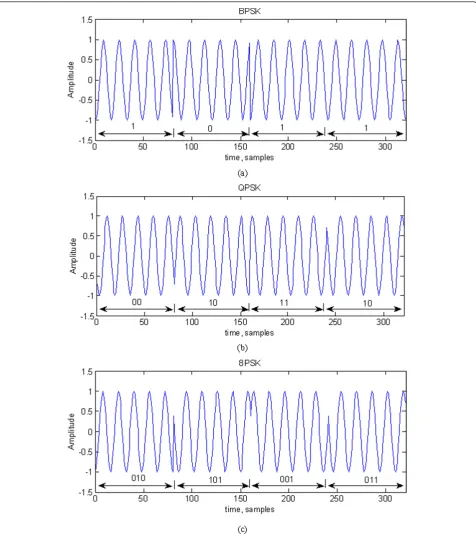
Figure 1 shows the time representations of the BPSK, QPSK, and 8PSK signals defined in Equation (4). The signal parameters are given in Table 1 and the sampling frequency is assumed to be 1 Hz. The analysis methods proposed in this article is applicable to communication applications in all frequency bands as long as they meet the Nyquist sampling theorem. Due to the frequency dependency of the S-transform, the analysis signals con-sist of both high- and low-frequency components so as to compare the performance of the AW-XWVD and S-transform for phase estimation.
The received noisy signal can be modeled as
y(t)=z(t) +v(t) (6)
where z(t) is the noiseless PSK signal and v(t) is the complex-valued additive white Gaussian noise. The noise has independent and identically distributed real and imaginary parts with total variance σ2
v and zero
2.2. TFDs, cross TFDs, and S-transform
The quadratic TFD is a useful technique to analyze time-varying signals, but the resulting TFR does not represent phase directly. Due to the need to estimate IIB-phase in PSK signals, the XTFD and the S-transform
are introduced for this purpose as both can represent phase in the time-frequency domain.
2.2.1. Quadratic TFDs and cross TFDs
represent the phase information in the time-frequency domain, the cross bilinear product in the XTFD is cal-culated using TFDs from both signal of interest and reference signal. The resulting formulation for the XTFD can be expressed as follows
ρzr(t,f) =
∞
−∞
G(t,τ)∗
(t)Kzr(t,τ) exp(−j2πfτ)dτ (7)
whereG(t,τ) is the time-lag kernel function that can also be represented in the Doppler-lag domain as described in [18,29]. The cross bilinear productKzr(t,τ)
is given as
Kzr(t,τ )=z t+ τ 2
r∗ t−τ
2
(8)
wherez(t) is the analytical signal of interest andr(t) is the reference signal. The cross bilinear product is the instantaneous cross correlation function (ICF) between the signal of interest and the reference signal. Similar to the signal of interest, the reference signal can be defined as
r(t) =A
N
k=1
expj2πfk(t−(k−1)Tb)
(t−(k−1)Tb) (9)
But it does not contain IIB-phase. A box function is used in the representation of the reference signal to keep track of the location of interaction between the signals of interest with the reference signal in the time-lag represen-tation. Similar study presented in [30,31] on the use of XWVD for IF estimate of linear FM signals requires a reference signal identical to the signal of interest. How-ever, this is not necessary for this application since the reference signal required is a pure sinusoid with the same frequency as the signal of interest. Hence, any power
spectrum estimation method [[32], p. 214] can be used to determine the frequency of the received signal. From there, a pure sinusoid reference signal of the same fre-quency is generated. This article assumes that the signal of interest is in perfect synchronization with the reference signal. In practical applications, the presence of phase syn-chronization error introduces an offset in the IIB-phase. This phase offset could be compensated using a PLL or Costas loop [33] to generate the reference signal. Further-more, the computation of the XTFD is done based on a segment of received signal. Combining the features of the PLL and Costas loop is only possible if the XTFD is com-puted iteratively one sample at a time.
In the general formulation of the quadratic TFD [[18], p. 68], the various TFD such as the Wigner-Ville distribu-tion (WVD), Choi-Williams distribudistribu-tion, spectrogram, B-distribution, and other distributions can be defined by their respective time-lag kernels. The choice of this kernel function can help minimize cross terms in the TFR. A separable kernel allows the flexibility to separately control the smoothing in the time and frequency domain [18, Sec-tion 5.7]. The kernel funcSec-tion for the windowed WVD (WWVD) is an example of a separable kernel. It performs smoothing only in the frequency direction to reduce the effect of the cross terms. Similar to the WWVD, the kernel function for the windowed XWVD (WXWVD) is defined as
G(t,τ)=δ(t)w(τ) (10)
Since the time component is a delta function, this ker-nel is independent of the Doppler variable and only a function of lag. The kernel is known as Doppler-inde-pendent kernel [[18], p. 71], a special case of separable kernel. It is shown that such kernel applies one-dimen-sional filtering and is adapted to only a particular kind
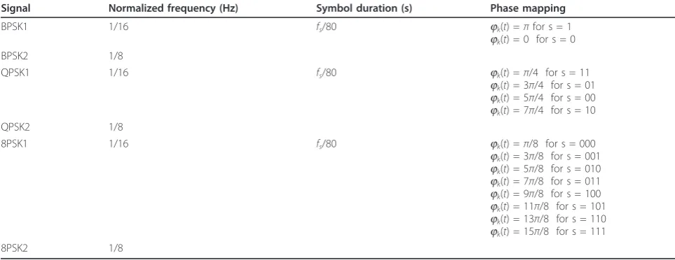
Table 1 Signal model parameters defined within a symbol duration
Signal Normalized frequency (Hz) Symbol duration (s) Phase mapping
BPSK1 1/16 fs/80 jk(t) =πfor s = 1
jk(t) = 0 for s = 0
BPSK2 1/8
QPSK1 1/16 fs/80 jk(t) =π/4 for s = 11
jk(t) = 3π/4 for s = 01
jk(t) = 5π/4 for s = 00
jk(t) = 7π/4 for s = 10
QPSK2 1/8
8PSK1 1/16 fs/80 jk(t) =π/8 for s = 000
jk(t) = 3π/8 for s = 001
jk(t) = 5π/8 for s = 010
jk(t) = 7π/8 for s = 011
jk(t) = 9π/8 for s = 100
jk(t) = 11π/8 for s = 101
jk(t) = 13π/8 for s = 110
jk(t) = 15π/8 for s = 111
of mono-component signals such as nonlinear FM sig-nals [[18], p. 214].Windowing is performed in the lag direction before taking the Fourier transform. Thus, the choice of separable kernel in Equation (10) causes smoothing only in the frequency direction.
By substituting Equation (10) into Equation (7), the WXWVD can be represented as
ρzr(t,f) =
∞
−∞
Kzr(t,τ)w(τ) exp(−j2πfτ)dτ (11)
The lag window functionw(τ) can be one of the win-dow functions typically used in filter design or spectrum analysis.
2.2.2. The S-transform
The S-transform is a spectral localization technique which is very much similar to the WT and STFT [24]. It can be considered as a special case of the STFT by replacing the window function with a frequency-depen-dent Gaussian window [24]. It is also related to the WT as it can be derived from the WT with a specific mother wavelet multiplied by the phase factor. The Gaussian window of the S-transform is scaled so that the window width is inversely proportional to the frequency, and its height is scaled linearly to the frequency. Due to the behavior of the window scaling, it possesses good time resolution for high-frequency components and good fre-quency resolution for low-frefre-quency components. This transform has successfully been applied for resolving problems in the field of geophysics [34], power quality analysis [35], and medicine [36]. The original formula-tion for the S-transform of a signal,z(t), is given as [24]
S(t,f) =
∞
−∞
z(τ)g(τ−t,f) exp(−j2πfτ)dτ (12)
The frequency-dependent Gaussian windowg(t, f) is given as [24]
g(t,f) = √f
2πexp
−
t2f2
2
(13)
wherefis the signal frequency and τin Equation (12) denotes the position of the midpoint of the window. The window spread or standard deviation depends onf. Based on the characteristics of the Gaussian distribution, a window width of 6/fensures that 99.72% of the signal values are enclosed within the window function [37]. Therefore, the window width is given as 6/fand height is given by the term f/√2π. The term f/√2π is also a normalizing factor which ensures thatS(t, f) con-verges toZ(f) when averaged over time [36], as shown below.
∞
−∞
S(t,f)dt=Z(f) (14)
Proof
∞
−∞ S(t,f)dt=
g(t−τ,f)z(τ) exp −
j2πfτdτdt
= f √ 2πexp
−(τ− t)2f2
2
z(τ) exp−j2πfτdτdt
= f √ 2πexp
−(τ− t)2f2
2
dtz(τ) exp−j2πfτdτ
= 1 √
2πexp
− u2 2 du 1
z(τ) exp−j2πfτdτ change of variable,u=(t−τ)f,du=fdt
=
z(τ) exp
−j2πfτdτ=Z(f)
Thus, the S-transform is invertible and the original signal can be recovered by taking the inverse Fourier transform of the above equation, resulting in the follow-ing expression ofz(t).
∞ −∞ ∞ −∞
S(t,f)dtexpj2πftdf=
∞
−∞
Z(f) exp(j2πft)df=z(t) (15)
3. Phase estimation methodology
This section describes the characteristics of the cross bilinear product in the time-lag representation and out-lines the derivation of the AW-XWVD. The adaptation method used to set up the localized lag adaptive window is then discussed. Next, the method used for phase esti-mation from the peak of the TFR is presented.
3.1. AW-XWVD
3.1.1. The cross bilinear product
The cross bilinear product consists of auto-terms and duplicated terms. The duplicated terms carry the same information as the auto-terms but shifted in time and lag domain; therefore, it can cause interference to the auto-terms [23]. In order to obtain an accurate XTFR, the auto-terms must be preserved and the duplicated terms must be removed or attenuated. The auto-terms and duplicated terms for any PSK class signal can be expressed as
Kzr,auto=
k=1
|A|2exp(j(2πfk+φk))K(t−(k−1)Tb,τ)(16)
Kzr,duplicated= N
k=1,k=l N
l=1
|A|2exp(j(2πf kτ) +φk)K
t−(k+l−2)Tb
2 ,τ (l−k)Tb
(17)
where K∏(t, τ) is the instantaneous autocorrelation function of the box function given as
K(t,τ )= t+τ 2
t−τ
2
(18)
The proofs for Equations (16) and (17) are given in Appendix 1.
In practical digital communication applications, the amplitude of the signal might not be ideally constant due to channel impairments such as multipath fading, attenuation by the propagation channel and any kind of amplification performed by the circuits at both the transmitter and receiver [13]. Therefore, the variableA is retained throughout the derivation of the cross bilinear product. Other than that, signals that combine amplitude and phase modulations such as QAM can also be used provided a suitable adaptation algorithm for the XTFD is designed. The variation in the ampli-tude,A, caused by the transmitted binary data will cor-respond to the variation in the energy represented in the XTFR.
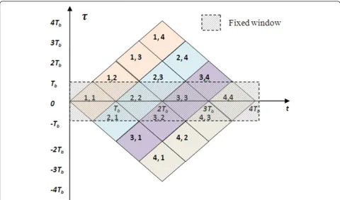
Figure 2 shows the graphical representation of the above cross bilinear product. All the auto-terms lie along theτ= 0 axis, whereas the duplicated terms are shifted in both time and lag. Therefore, the terms labeled asKzr1,2, Kzr1,3, andKzr1,4are the duplicated terms for the
auto-term,Kzr1,1, which are centered atτ= 0 axis. The same
label applies to the rest of the auto-terms and duplicated terms. The following examples illustrate the problem caused by the duplicated terms to the estimation of IIB-phase. There is no interference observed in the IIB-phase estimate if there are only auto-terms present. For instance, at timet=Tb/2 the cross bilinear product
eval-uated is given as
Kzr(t,τ)|t=Tb/2=A
2exp(j(2πf0τ+φ1)) (τ+T
b) (19)
Only the auto-terms with the IIB-phase of 1 exist.
When both the auto-terms and duplicated terms are present, there will be more than one phase term. This is observed at t=3Tb/2 where the cross bilinear product
is represented as
Kzr(t,τ)t=3Tb/2=A 2[exp(j(2πf
0τ+φ3))(τ+ 3Tb) + exp(j(2πf0τ+φ2))(τ+Tb)
+ exp(j(2πf0τ+φ1))(τ−Tb)] (20)
The interaction of the auto-terms and duplicated terms can be visualized as the addition of multiple vec-tor components which result in a new vecvec-tor compo-nent with different magnitude and phase. Instead of IIB-phase of 2 which is caused by the auto-terms, the
resulting IIB-phase consists of the interaction between all the phase terms1 and3 caused by the duplicated
terms.
Since all auto-terms lie along theτ = 0 axis, a fixed width lag window was used in [23] to preserve the auto-terms and partially remove the duplicated auto-terms that cause distortion in the IIB-phase represented on the XTFR. However, success is limited because the dupli-cated terms are not completely removed resulting in a distorted IIB-phase estimate. To resolve this problem, the fixed lag windoww (τ) in Equation (11) is replaced with a time-dependent window functionw(t,τ) and the resulting new TFD, known as the AW-XWVD, is given as
ρzr,AWXWVD(t,f) =
∞
−∞
Kzr(t,τ)w(t,τ) exp(−j2πfτ)dτ(21)
The adjustment of this time-dependent window width is based on the computation of the LLAC function at every time instant to separate the auto terms and dupli-cated terms. This is equivalent to use a separable kernel to reduce all cross terms as shown in [21,22]. An analy-sis window centered at τ = 0 is used as a reference to perform the similarity test using the LLAC function. This similarity test detects the variation of the signal in the lag direction at every time instant and estimates the window width. The time-dependent window function can be implemented using one of the common windows used in digital filter design and spectrum estimation. In this application, a rectangular window is used and it can be defined as
w(t,τ) =
1 −τg(t)≤t≤τg(t)
0 elsewhere (22)
where τg (t) is the time-dependent window width
estimated accordingly. The desired τg(t) in the positive
lag (or in the negative lag direction) is selected if
τg(t)= min
ς (|RKK(t,ς)|)
0< ς ≤T,
−T≥ς >0, (23)
whereςis the time instant in lag and |RKK(t,ς)| is the
amplitude of the LLAC which will be discussed in the following section. Note that the rectangular window was used for simplicity as we observed that the proposed methodology performance is not affected significantly by the choice of the window shape.
3.1.2. Adaptation algorithm
The LLAC [20] of the kernel, K, is a function of time and lag and it can be defined as
RKK(t,ς) = T
−T
wa(τ)2Kzr(t,τ)Kzr(t,τ−ς)dτ (24)
where wa (τ) is the analysis window, τ is the lag
instant, and ςis the lag running variable. The possible range for the normalized LLAC amplitude is
0≤RKK(t,ς)≤1 (25)
A higher value of the amplitude of the LLAC function implies that the similarity is high and vice versa. The
miscorrelation in the signal is indicated by a drastic drop in the amplitude of the LLAC function. The LLAC function will give a value approaching unity at lag instant,ς= 0.
The analysis window is a parameter of the LLAC. Its selection is important to ensure that the LLAC can detect the variation along the lag axis based on the condition spe-cified in Equation (23) as to estimate the time-dependent window width. The analysis window is defined as
wa(τ)= 1
τa
0< τa<<T (26)
where τais the analysis window width. In this article,
the analysis window width is chosen experimentally as
τa= 10 s based on the sampling frequency of 1 Hz. The
LLAC is applied to the signalx(t) and evaluated for the normalized frequencies of 1/32, 1/16, 1/8, and1/4 Hz. In this evaluation, the signal is defined as follows (with similar characteristic to the cross bilinear product in lag)
x(t) = exp(j2πf1t) 0≤t≤Tb
= exp(j2πf1(t−Tb)) exp(jπ) Tb≤t≤2Tb
(27)
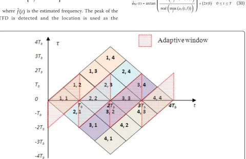
Table 2 shows the minimum values of the LLAC evalu-ated in time. An analysis window ofτa= 10 s is sufficient
frequencies ranged from 1/32 to 1/4 Hz. Thus, the analysis width is valid for the test signals as specified in Section 2. In the case of PSK signals, two consecutives symbols may be different from each other depending on the transmitted data. By applying the LLAC on the cross bilinear product, the resulting adaptive window resembles the shape of a parallelogram as shown in Figure 3.
3.2. IIB-phase estimation from the peak of TFDs
By extending the approach used for IF estimation from the peak of WVD presented in [26], the IIB-phase is estimated frrm the peak of the AW-XWVD and S-trans-form as outlined in the following sections.
3.2.1. IIB-phase estimation using the AW-XWVD
The IF can be estimated from the peak of the TFD for all time instants as shown below [[18], p. 429]
ˆ
f(t) = arg
max f
ρz(t,f)
, 0≤t≤T (28)
where fˆ(t) is the estimated frequency. The peak of the TFD is detected and the location is used as the
frequency estimate. In this application, the peak of the XTFD for the AW-XWVD is detected for all time instants and it is used to estimate the phase. Since the peak value is complex, the IIB-phase may be expressed as the inverse tangent of the imaginary and real compo-nent, that is
ˆ
φAWXWVD(t)= arctan ⎛ ⎜ ⎜ ⎝
imag
max
f
ρzr
t,f
real
max
f
ρzrt,f
⎞ ⎟ ⎟
⎠ 0≤t≤T (29)
The detailed derivation of the above equation is given in Appendix 3.
3.2.2. IIB-phase estimation using the S-transform
For the S-transform, the IIB-phase estimation from the peak of the TFD, however, is not as straightforward as the AW-XWVD. The phase term in the frequency repre-sentation introduced by the time shift window has to be compensated in the actual IIB-phase estimate. The rela-tionship between the time delay and phase shift is pre-sented in [40], where the authors utilized this property to generate the analytical signal as an alternative to the Hil-bert transform. By applying this concept, the estimated IIB-phase using S-transform can be represented as
ˆ
φST(t)= arctan
⎛ ⎜ ⎜ ⎝
imag
max f
ρz
t,f
real
max f
ρz
t,f ⎞ ⎟ ⎟
⎠+2πft 0≤t≤T (30)
Table 2 Minimum Value of LLAC for various frequencies
Number Signal frequency (Hz) Min |RKK(t,ς)|
1 1/32 0.567
2 1/16 0.251
3 1/8 0.121
4 1/4 0.089
The detailed derivation for IIB-phase estimation using S-transform is given in Appendix 4.
3.3. Comparison to CRLB
This section compares the performance of both AW-XWVD and S-transform as a phase estimator with the CRLB which is often used as a benchmark [41], as it gives the theoretical lower limit to the variance of any unbiased parameter estimator [42]. The CRLB derived in [43,44] uses a likelihood function on a known signal in the presence of additive white noise for the digitally phase modulated signal.
In terms of SNR, the CRLB for BPSK and QPSK sig-nals can be represented, respectively, as [43]
CRBB(φ)=
1
2NγFB
1
γ
(31)
CRBQ(φ)=
1
2NγFQ
1
γ
(32)
whereNis the average window width,gis the SNR,FB
andFQare, respectively, the ratio of the CRLB for
ran-dom BPSK and QPSK signals to the CRLB for an unmo-dulated carrier of the same power. At high SNR, the value ofFBand FQ is equivalent to one; so, the same
bound applies for both the BPSK and QPSK signals [43]. The value of FBandFQdiffers at low SNR and is
obtained from the results presented in [43]. In [44], the authors extended the study presented in [43] and derived the CRLB for 8PSK signal with random phase. It is shown that the CRLB for MPSK signal for moderate to low SNR is given as [44]
CRBMPSK(φ)=
1
2Nγ (33)
The variance of the actual IIB-phase estimator for both AW-XWVD and S-transform method can be represented as
var (φˆ) = 1
N N−1
n=0
ˆ
φn− ¯φ
2
(34)
where N is the total number of samples, φˆn is the estimated phase at every time sample n, and φ¯ is the actual IIB-phase.
3.4. PSK signal detection algorithm
In addition to the estimation of modulation parameters, the IIB-phase estimate derived from the XTFR can also be used as a demodulator for the class of PSK signals.
The detection is performed by first estimating the IIB-phase, (t) from the peak of the TFD. The average IIB-phase within a symbol duration can be estimated as fol-lows
¯
φ= 1
Tb Tb
0
ϕ(t)dt (35)
For a BPSK signal, the symbols are detected based on a set of decision rule [45] that are defined as
sBPSK=
⎧ ⎪ ⎨ ⎪ ⎩
0 − π
2 ≤ ¯φ <
π
2
1 π
2 ≤ ¯φ <−
π
2
(36)
wheresBPSKis the estimated binary data. The decision
boundary is defined based on the signal parameters shown in Table 1. Similarly, the same approach described for BPSK is extended to QPSK and 8PSK. The decision rule for QPSK and 8PSK signals are defined, respectively, as
sQPSK=
⎧ ⎪ ⎪ ⎪ ⎪ ⎪ ⎪ ⎨ ⎪ ⎪ ⎪ ⎪ ⎪ ⎪ ⎩
11 0≤ ¯φ < π 2
01 π
2 ≤ ¯φ < π 00 π≤ ¯φ <−π
2
10 − π
2 ≤ ¯φ <0
(37)
s8PSK=
⎧ ⎪ ⎪ ⎪ ⎪ ⎪ ⎪ ⎪ ⎪ ⎪ ⎪ ⎪ ⎪ ⎪ ⎪ ⎪ ⎪ ⎪ ⎪ ⎪ ⎪ ⎨ ⎪ ⎪ ⎪ ⎪ ⎪ ⎪ ⎪ ⎪ ⎪ ⎪ ⎪ ⎪ ⎪ ⎪ ⎪ ⎪ ⎪ ⎪ ⎪ ⎪ ⎩
000 0≤ ¯φ < π 4
001 π
4 ≤ ¯φ <
π
2
011 π
2 ≤ ¯φ < 3π
4
010 3π
4 ≤ ¯φ < π 110 π≤ ¯φ <−3π
4
111 −3π
4 ≤ ¯φ <−
π
2
101 −3π
4 ≤ ¯φ <−
π
2
100 −π
2 ≤ ¯φ <0
(38)
4. Implementation, results, and discussions
a phase estimator is benchmarked to the CRLB. This is followed by the evaluation of the symbol error rate per-formance of the AW-XWVD, S-transform, and conven-tional detector. Finally, a comparison is made in terms of the computational complexity between the AW-XWVD, S-transform, and conventional detector.
4.1. Discrete-time formulation and implementation
The discrete time formulation of the TFDs is needed for implementation on digital systems; and this applies for both the discrete forms of the AW-XWVD and S-trans-form. In [[18], p. 235], the windowed discrete WVD (DWVD) of a continuous-time signalz(t) is expressed as
Wzn,k= 2
|m|≺M/2
w[m]z[n+m]z∗[n−m]exp(−2πkm/M) (39)
where M is a positive integers representing the win-dow length in samples,nis the discrete time samples, m is the discrete lag samples, and k is the discrete fre-quency. Thus, by using Equation (21), the discrete AW-XWVD can be expressed as
ρzr,AWXWVD,n,k= 2
|m|<M/2
w[n,m]z[n+m]r∗[n−m]exp(−2πkm/M) (40)
Using the same notation as above, the discrete S-transform [24] can be represented as
Sn,k= M−1
m=0 z(m)√|k|
2πexp
−(m−n)2k2
2
exp(−j2πkm/M) (41)
The discrete time representation of the S-transform is similar to the spectrogram. However, there is a tradeoff between the time and frequency resolution for the S-transform as the window width is frequency dependent.
4.2. Results
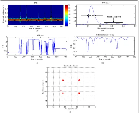
Figures 4 and 5 show the TFR, TFR slice, IIB-phase, instantaneous energy, and constellation plots for QPSK2 signals at SNR of 10 dB using the AW-XWVD and S-transform, respectively. The two TFRs show at which fre-quency the signal exists, but for the S-transform there are distortions in the TFR at every symbol transition. The high contrast region in the TFR of the S-transform indi-cates that there are low-density components other than the signal component. However, this is not present in the TFR of the AW-XWVD. The TFR slice is normalized to the peak value of the TFR and observed in frequency for timen= 100 samples. From the TFR slice, it is shown that the AW-XWVD gives better frequency concentra-tion compared to the S-Transform. This is because the MLW of the TFR slice for the S-transform appears to be much wider than AW-XWVD. As shown in Equation (12), the S-transform’s window width is frequency
dependent where the window is wider for low-frequency signal and narrower for high-frequency signal. This implies that the S-transform at higher frequency gives worse frequency resolution and wider MLW. Results confirming this statement are presented in Table 3. Besides the MLW of the TFR slice, there is also a differ-ence in the average side lobe level. The side lobe level is higher for the S-transform at about 0.18, while this level is lower at 0.05 for the AW-XWVD. This explains the appearance of the high contrast region on the TFR of the S-transform.
The IIB-phase plot shows that the AW-XWVD gives better accuracy for the IIB-phase estimate. For the S-transform, distortion is observed in the IIB-phase esti-mate at the phase transition regions which is absent in the AW-XWVD. The sliding window in the S-transform causes distortion in the IIB-phase at the symbol transi-tion region due to the interactransi-tion between adjacent symbols. Since digitally phase modulated signals have constant amplitude, their instantaneous energy should also be constant at all times. However, due to noise, the amplitude of the signal appears to vary. This is reflected as variation in the magnitude of the instantaneous energy for AW-XWVD and S-transform. A significant drop is observed in the instantaneous energy for the S-transform at every symbol transition. Similar to the phase, this drop is caused by the interactions between the adjacent symbols within the sliding window. Since the AW-XWVD produces accurate instantaneous energy and IIB-phase estimates, the constellation diagram gen-erated shows almost no variation from the original points and is better compared to the S-transform. Table 3 shows the MLW estimated at SNR of 6and 10 dB using both methods. In general, the SNR has no signifi-cant effect in the MLW obtained for both methods. However, the effect of signal frequency is more signifi-cant for the S-transform compared to the AW-XWVD. For instance, the MLW for both BPSK1 and BPSK2 with the AW-XWVD based estimate is the same at 0.012 Hz. However, for the S-transform the MLW is lar-ger for BPSK2 than BPSK1 with a difference of 0.028 Hz. The scaling of the Gaussian window results in a broader MLW for higher-frequency signal. The signal modulation level has no significant effect on the MLW. This is shown by the MLW measured for BPSK, QPSK, and 8PSK signals where there are only minor differ-ences. These results imply that the AW-XWVD gives better IIB-phase estimation results compared to the S-transform as the performance of an estimator is asso-ciated with the MLW [[46], p. 50].
4.3. Variance comparison with the CRLB
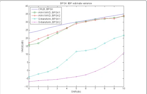
methods are benchmarked with the CRLB for phase esti-mate. It is assumed that there is perfect synchronization between the received and reference signals. We consider the signal is corrupted by a zero mean additive white Gaussian noise channel with variances2. In simulations, the received signal is generated by adding the noiseless signal,z(t), and the additive white Gaussian noise,v(t), as given in Equation (6) where the SNR is varied at 1 dB step from 0 to 10 dB. Monte Carlo simulations based on 1,000 realizations of the predefined signals are conducted for each value of SNR. The estimated IIB-phase is obtained from the peak of the XTFD as described in Sec-tion 3.2. Assuming the actual IIB-phase of the signal is known, the MSE is computed using Equation (34). Fig-ures 6, 7, and 8 show the results of the estimated IIB-phase variance for BPSK, QPSK, and 8PSK signals, respectively. In general, for both BPSK and QPSK signals,
the variance of IIB-phase estimate using the AW-XWVD lies close to the CRLB. The AW-XWVD estimate meets the CRLB at SNR≥5 dB for both BPSK1 and BPSK2 sig-nals. Figure 7 shows that the cutoff point for both QPSK1 and QPSK2 signals are the same as the BPSK sig-nals, at SNR of 5 dB. However, the variances in the IIB-phase estimate for QPSK signals are higher compared to the BPSK signals at the same SNR. A higher cutoff point is recorded for the 8PSK estimates where both 8PSK1 and 8PSK2 signals meet the CRLB at SNR≥7 dB. In gen-eral, the AW-XWVD outperformed the S-transform as a phase estimator and the S-transform estimates never meet the CRLB for all signals even at SNR of 10 dB. As expected, the performance of the S-transform deterio-rates greatly for higher frequency signals due to broader MLW. This is in contrast with the AW-XWVD where it maintains reasonably insignificant changes in the Figure 4QPSK2 signal evaluated using AW-XWVD at SNR = 10 dB: (a) TFR (b) TFR slice (c) IIB-phase, (d) Instantaneous energy (e)
variance of IIB-phase estimates for all range of frequency. Thus, the AW-XWVD is more robust to noise for phase estimation compared to the S-transform. The result obtained in this article is in line with [30] where the XWVD is shown to be more robust to noise compared to the WVD.
4.4. Symbol error rate performance
In this section, the symbol error rate performance of the AW-XWVD and S-transform is compared with the con-ventional detector defined in [[13], p. 188] for the class of PSK signals. It is based on the matched filter struc-ture, where the reference signal must have the same parameters as and be in phase with the signal of inter-est. In general, an increment in the number of bits per symbol will increase the throughput at the expense of downgrading the symbol error rate. The formulation for Figure 5QPSK2 signal evaluated using S-transform at SNR = 10 dB: (a) TFR (b) TFR slice (c) IIB-phase (d) Instantaneous energy (e)
Constellation diagram.
Table 3 Performance comparison between AW-XWVD and S-transform
SNR Signals MLW (Hz)
AW-XWVD S-Transform
6 dB BPSK1 0.012 0.025
BPSK2 0.012 0.053
QPSK1 0.016 0.025
QPSK2 0.015 0.046
8PSK1 0.017 0.031
8PSK2 0.017 0.052
10 dB BPSK1 0.010 0.023
BPSK2 0.010 0.049
QPSK1 0.014 0.024
QPSK2 0.014 0.0486
8PSK1 0.015 0.029
the symbol error rate for coherently detected multiple phase modulation signals is given as [[13], p. 229]
PE(M)≈2Q
2Es N0
sinπ
M
(42)
wherePE(M) is the symbol error rate, the functionQ(x)
is the complementary error function,Esis the energy per
symbol,N0is the noise power, andMis the size of
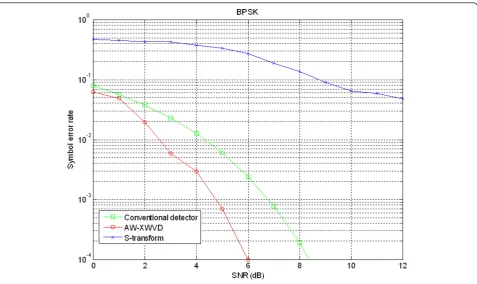
sym-bol set. Detection of the PSK signals is done based on the IIB-phase estimate and the sets of rules defined in Sec-tion 3.4. All the defined test signals of 10,000 symbols are evaluated under AWGN channel. The results presented in Figures 9, 10, and 11 show the symbol error rate per-formance as a function of SNR for BPSK, QPSK, and 8PSK signals. BPSK signal required a SNR of about 5 dB to achieve a symbol error rate of 10-3 for the AW-XWVD method. Using the same method, a higher SNR is observed for QPSK signal, approximately 8 dB. To achieve the same performance, the conventional detector needs an SNR of 7 and 8 dB for BPSK and QPSK signals, respectively. For 8PSK signal, it is shown that to achieve a symbol error rate of 10-3, SNR of 10 dB is required for AW-XWVD. As for the conventional detector, it gives the same performance at SNR of 11 dB. From the symbol
error rate plot, for all the test signals, it is observed that the advantage of the AW-XWVD over the conventional detector is at the low SNR range where it gives lower error rate. In general, the symbol error rate for the AW-XWVD is much lower compared to the S-transform. The S-transform could not provide symbol error rate≤10-3 even at SNR of 12 dB for all signals. Thus, it is impracti-cal to use it as a detector for the class of PSK signals.
4.5. Computation complexity
The number of computations for implementing the AW-XWVD, the S-transform, and conventional detectors is discussed in this section to compare the practicality of the proposed method for signal analysis and classification applications as used in spectrum monitoring and cogni-tive radio [14-17]. The computation complexity of the AW-XWVD is similar to the smooth WWVD due to the similarity in the computation of the bilinear product. To implement the AW-XWVD, the number of computation required in terms of the number of multiplication is given below [22]. For the sake of clarity in terminology, in the paragraph below,Nis the signal length,Nτis the lag window length, NA is the length of the analysis
window, and Nw is the average length of adaptive lag
Figure 7QPSK IIB-phase estimate variance.
1. Computation of the cross bilinear product to obtain its time-lag representation requires NτN
mul-tiplications. Ideally, the number of computation for the cross bilinear product is N2 where the lag and time durations are equal to Nsamples. To maintain equal frequency resolution forN> 512 samples, the duration in lag is maintained at Nτ= 512 samples.
By limiting the duration in lag, excessive computa-tion of the cross bilinear product is avoided.
2. The LLAC uses an analysis window of NAwhich
slides along the lag axis at every lag sample for a total of Nτsamples. Since there areNtime instances, the total number of multiplications for the computa-tion of localized lag autocorrelacomputa-tion funccomputa-tion is NANτN.
3. The LLAC will determine the separation interval between the auto-terms and duplicated terms based on the average lag window width Nw. For N time
samples, the total number of multiplications to setup the adaptive lag window based on the average lag window widthNwis NwN.
4. To get the XTFR, the Fourier transform of the windowed cross bilinear product is calculated in the lag direction with (Nτlog2 Nτ) multiplications. For
signal length N, the total number of multiplications 0.5N(Nτlog2Nτ).
Therefore, the total of multiplication required to com-pute the AW-XWVD isN(Nτ+NANτ+Nw + 0.5Nτlog2 Nτ).
The S-transform is very much similar to the spectro-gram, except that the window for the S-transform is fre-quency dependent. Hence, the number of computation required in terms of number of multiplication results from [47]:
1. The product of the frequency-dependent Gaussian window function and the signal of interest to obtain its localized spectrum which requires N multiplications.
2. The Fourier transform of the time-lag representa-tion to obtain the TFR requires 0.5N(Nτlog2 Nτ)
multiplications.
Thus, the total number of multiplication required to implement the S-transform isN(1 + 0.5Nτlog2Nτ).
The number of computation in terms of the number of multiplication required to implement the conven-tional detector is [13]:
1. Mixing of the incoming signal with two sinusoid signals with 90° phase difference requires 2N multiplications.
Figure 10BER performance for QPSK signal in AWGN channel.
2. Low pass filtering of the signal to obtain the inphase and quadrature phase component of the sig-nal require 2Nmultiplications.
Therefore, the total number of multiplications required to implement the conventional detector is 4N.
In this application, the length of the signal evaluated is 640 samples points and the lag window lengthNτis set to 512 sample points. The analysis window lengthNA
used in the AW-XWVD is 10 samples points and the average length of adaptive lag windowNw is 80 samples
points. The number of multiplications required for the AW-XWVD, S-transform, and conventional detector per symbol is summarized in Table 4.
In terms of the number of multiplications, the AW-XWVD requires approximately 4 times more computa-tions compared to the S-transform and 2,000 times more for the conventional detector. Although there is a significant additional number of a computation for the AW-XWVD, recent advances in digital electronics as well as decimation procedures can take care of them; in addition, the performance in terms of the IIB-phase esti-mates enables more efficient signal parameters estima-tion in the proposed area of applicaestima-tions. These parameters can be used to classify a signal from a set of reference parameters. If necessary, we can use the IIB-phase estimate to detect PSK signals at low SNR condi-tions where the conventional detector failed. For higher SNR conditions, it is not necessary to use a technique which is computationally intensive when the symbol error rate is low. Thus, we can setup the conventional detector using the parameters estimated from the IIB-phase to detect PSK signal. So, we conclude that, with the enhancement of current computer processing com-bined with appropriate decimation procedures, the real-time implementation of AW-XWVD is feasible with the use of multiple processors or parallel processing [48] and the design proposed in [49].
5. Conclusions
A performance comparison between the AW-XWVD and S-transform estimators of IIB-phase shows that the AW-XWVD is superior to the S-transform for classify-ing PSK signals. Results show that the mean square
error of the phase estimate using AW-XWVD is on the average lower by 20 dB. The S-transform has a fre-quency-dependent window width which performs poorly as a phase estimator for high-frequency signal compo-nents. Since peak detection is used for the estimation of the IIB-phase for both methods, the frequency resolu-tion and MLW contribute to the estimaresolu-tion accuracy. The AW-XWVD maintains the frequency resolution through the window adaptation and yields better accu-racy for the IIB-phase estimate. It also meets the CRLB at moderate SNR for all the defined signals unlike the S-transform that never meets the bound even at high SNR. For symbol error rate performance, the AW-XWVD is also better compared to the S-transform and it is comparable to the conventional detector at the cost of higher number of computations. Thus, this article has proven that the AW-XWVD is an effective phase esti-mator for digitally phase modulated signals and can be used for similar applications involving time-varying sig-nals. This study suggests new research directions to pur-sue in the future, such as replacing the S-transform by a modified S-transform that incorporates an adaptive mechanism; replacing the transform by the cross S-transform; using separable kernels in defining a XTFD; and investigate the effect of window shape in Equation (40) on the performance of the phase estimator. These advances can be used in a wide range of signal proces-sing applications from Telecommunications to Biomedi-cine including EEG and Fetal Movement signals analysis and processing, where time-frequency peak detectors can provide additional features for classification improvement.
Endnote a
The terminology“duplicated terms” is used in this arti-cle instead of the cross terms which is typically used in TFA. This is because, in the proposed method, these terms carry the same information as the auto-terms but are shifted in both time and lag. The duplicated terms are caused by the cross bilinear product between thekth and lth symbol of the signal of interest and the refer-ence signal, wherek≠l.
Appendix 1. Derivation of the auto-terms
Derivation of the auto-terms will be discussed in this section. Cross bilinear product can be seen as the results of the cross correlation function between the signal of interest and a reference signal. For discussion purposes, a PSK signal of N symbols length with normalized amplitude is evaluated. The signal has the same fre-quency and the difference between each symbol is the phase that is determined by the binary information pre-sent. The N symbol length PSK signal can be repre-sented as
Table 4 Comparison of computational complexity between AW-XWVD, S-transform and the conventional detector
Methods of IIB-phase estimation
Number of multiplication per symbol
AW-XWVD 6.41 × 10⁵
S-transform 1.84 × 10⁵
z(t) =
N
k=1
expj2πf0
t−(k−1)Tb
+φk
(t−(k−1)Tb)
= expj2πf0t+φ1(t)
(t) + expj2πf0(t−Tb)+φ2(t−Tb)
(t−Tb)
+ expj2πf0(t−2Tb)+φ3(t−2Tb)
(t−2Tb)
+ expj2πf0(t−3Tb)+φ4(t−3Tb)
(t−3Tb)+· · ·
+ expj2πf0
t−(N−1)Tb
+φN
t−(NTb
t−(N−1)Tb
(A:1)
The reference signal with respect to the signal of interest is given as
r(t) =
N
k=1
expj2πf0(t−(k−1)Tb)
(t−(k−1)Tb)
= expj2πfot
(t)+ expj2πfo(t−Tb)
(t−Tb)
+ expj2πfo(t−2Tb)
(t−2Tb)+ exp
j2πfo(t−3Tb)
(t−3Tb)+· · ·
+ expj2πfo
t−(N−1)Tb
t−(N−1)Tb
(A:2)
Substituting Equations (A.1) and (A.2) into Equation (8) then the cross bilinear product is given as
Kzr(t,τ) = N
k=1
exp j2πf0 t+τ 2−(k−1)Tb
+φk
t+τ
2−(k−1)Tb
× N
l=1
exp −j 2πf0(t−τ
2−(l−1)Tb)
t−τ
2−(l−1)Tb (A:3)
Here, the auto-terms are defined as the cross bilinear product between the signal of interest and the reference signal at the same time instant the box function over-laps a copy of itself. For instance, the ICF of the first symbol with the reference signal at the same time instant, wherek=l= = 1, can be represented as
Kzr,1,1(t,τ) = exp
j2πf0τ+ϕ1
t+τ
2
t−τ
2
(A:4)
For the second symbol, the ICF of the signal and reference signal occurring at the same time, wherek=l = 2, is given as
Kzr,2,2(t,τ) = expj2πf0τ+ϕ1 t−Tb+τ 2
t−Tb−τ 2
(A:5)
The cross bilinear product assembled a rhombic shape and the IAF of the box function given in Equation (18) has a maximum value when they overlap by a copy of itself. This condition applies when the shift in lag is zero. To simplify the notation of the IAF of the box function, the beginning point of each IAF of the box function is determined. For example,
(a) K,1,1(t,τ) = t+τ
2
t− τ
2
t+τ
2 =t−
τ
2
τ = 0
(A:6)
Then substitutingτ= 0 into the box function,
t+0 2
t−0
2
= (t) (t) (A:7)
From Equations (A.6) and (A.7), the IAF of the box function can be represented as K∏ (t, τ) where this bilinear product begin att =0 andτ= 0.
(b) K,2,2(t,τ) = t−Tb+τ 2
t−Tb−τ 2
t−Tb+τ
2 =t−Tb−
τ
2
τ = 0
(A:8)
Substituteτ= 0 into the box function,
t−Tb+
0 2
t−Tb−
0 2
= (t−Tb) (t−Tb) (A.9)
Then, the IAF for box function for the second auto-term can be represented as K∏ (t-Tb, τ) where it is
shifted byt=Tbin the time domain and shifted byτ=
0 in lag domain.
From Equations (A.6) to (A.9), a general representa-tion for the auto-terms is given as
Kzr,auto(t,τ )=
N
k=1
|A|2expj2πf
k+φk
K(t−(k−1)Tb,τ)(A:10)
The above equation shows that all the auto-terms are located along the time axis at τ= 0 and carry the IIB-phase for each symbol. Each individual auto-term has a rhombic shape and begins att=kTb.
Appendix 2. Derivation of the duplicated terms
In this section, the derivation of the duplicated terms is discussed using the same test signal defined in Appendix 1. The duplicated terms are the cross bilinear product between the kth andlth symbol of the signal of interest and the reference signal, wherek≠l. The cross bilinear product between the first and second symbols are given as
Kzr,1,2(t,τ )= exp j2πf0 t+τ 2
+φ1
t+τ 2−Tb
·exp−j2πfo t−τ2t−τ2
= expj2πf0τ+φ1K
t−Tb
2,τ−Tb
(B:1)
It is observed that this term has the same frequency and IIB-phase content as theKzr,1,1 (t,τ) auto-term but
is shifted in both time and lag.
Kzr,2,1(t,τ )= exp j2πf0t+τ2
+φ2
t−τ2·exp −j2πfo t−τ2
t−τ2−Tb
= expj2πf0τ+φ2
K
t−Tb
2,τ+Tb
(B:2)
Kzr,duplicated(t,τ)=
N
k=1
k=l N
l=1
|A|2expj2πf
kτ+φk
K
t−(k+l−2)Tb
2 ,τ−(l−k)Tb
(B:3)
The above indicates that the signal power, frequencies, and IIB-phase for the duplicated terms are the same as the auto-terms except that they are shifted in both time and lag. It has a rhombic shape and it begins at
t= (k+l−2)Tb
2 and τ= (l - k)Tb
Appendix 3. Phase estimation from the peak of XWVD
This section represents the derivations for phase estima-tion from the TFR generated by the XWVD. Similar to Appendix 1, the derivations consider a 4-symbol digital phase modulation signal that is defined in Equation (A.1). The derivation is first presented for the AW-XWVD followed by the S-transform. With reference to Appendix 1 and Section 3, it is assumed that the adapta-tion algorithm has completely preserved the auto-terms and part of the duplicated terms that do not cause dis-tortion in the IIB-phase estimate. The explanation is simplified by considering the cross bilinear product for att = 3/2Tband t= 5/2Tband the cross bilinear
pro-duct evaluated over lag over these time instants are
Kzr(3/2Tb,τ) = exp(jϕ2) exp(j2πf1τ)(τ) (C:1)
Kzr(5/2Tb,τ) = exp(jϕ3) exp(j2πf1τ)(τ) (C:2)
where the box function is defined as
(τ) = 1, 0≤τ ≤ Tb
= 0 elsewhere (C:3)
To obtain the XTFR, the Fourier transform is evalu-ated in lag according to Equation (21) and the resulting XTFR at these time instants are
ρzr(3/2Tb,f) =FT τ→f
Kzr(3/2Tb,τ)
= exp(jϕ2) sinc(f1−f) (C:4)
ρzr(5/2Tb,f) = FT τ→f
Kzr(5/2Tb,τ)= exp(jϕ3) sinc(f1−f) (C:5)
The results show that cross TFR at both time instants is maximum at the frequency off1 but the peak values
are determine by the IIB-phase of2 and3. Instead of
using the peak of TFR to determine the IF as described in [22,25,28], the peak value is used to estimate the IIB-phase. Since the peak value is complex, the IIB-phase for both time instances can be estimated as follows
ˆ
φAWXWVD
3/2Tb = arctan ⎛ ⎜ ⎜ ⎝ imag max f ρzr
3/2Tb,f real max f ρzr
3/2Tb,f
⎞ ⎟ ⎟ ⎠= arctan
imagexp(jφ2)
realexp(jφ2)
= arctan
sin(φ2)
cos(φ2)
=φ2
(C:6)
ˆ
φAWXWVD
5/2Tb = arctan ⎛ ⎜ ⎜ ⎝ imag max f ρzr
5/2Tb,f real max f ρzr
5/2Tb,f
⎞ ⎟ ⎟ ⎠= arctan
imagexp(jφ3)
realexp(jφ3)
= arctan
sin(φ3)
cos(φ3)
=φ3
(C:7)
By extending this formulation to all time instants, the IIB-phase estimate is
ˆ
φAWXWVD(t)= arctan ⎛ ⎜ ⎜ ⎝ imag max f ρzr
t,f
real max f ρzr
t,f
⎞ ⎟ ⎟
⎠(C:8)
The above indicates that the accuracy of the IIB-phase estimate depends greatly on the XTFR. Therefore, the duplicated terms must be removed to produce an opti-mal XTFR, in which we employ an adaptive window as a kernel function to preserve the auto-terms and attenu-ate the duplicattenu-ated terms.
Appendix 4. Phase estimation from the peak of S-transform
For the S-transform, the similar signal model described in Equation (A.1) is used and the TFR is calculated using Equation (12). Similar to the XTFD, the TFR for the signal using the S-transform is first calculated at time instants oft= 3/2Tbandt= 5/2Tbbefore the
IIB-phase estimate formulation is derived. Att= 3/2Tb, the
window function g(t) covers within the second symbol of the digital phase modulation signal and the substitu-tion of Equasubstitu-tion (4) into Equasubstitu-tion (12) results in
S(3/2Tb,f) = ∞
−∞
exp(jφ2) exp(j2πf1(τ−Tb))(τ−Tb)g(τ−3/2Tb) exp(−j2πfτ)dτ (D:1)
The time shift window in the S-transform introduces a phase term in the frequency representation which is described as follows by the time shift properties of the Fourier transform
FT
τ→f
g(τ−t)⇒exp−j2πftG(f) = exp−jφG(f) (D:2)
By including this effect, the TFR for the signal is obtained by evaluating Equation (D.1) is given as
S(3/2Tb,f) = exp(jϕ2) exp
−j2πf1 3 2Tb
G(f−f1)(D:3)
whereG(f - f1) is the frequency representation of the
window evaluated at the frequency of f1. Due to the