Representing time-dependent freezing behaviour in immersion mode ice nucleation

www.atmos-chem-phys.net/14/8501/2014/ doi:10.5194/acp-14-8501-2014

© Author(s) 2014. CC Attribution 3.0 License.

Representing time-dependent freezing behaviour in immersion

mode ice nucleation

R. J. Herbert1, B. J. Murray1, T. F. Whale1, S. J. Dobbie1, and J. D. Atkinson1,* 1_{School of Earth and Environment, University of Leeds, Leeds, LS2 9JT, UK}

*_{now at: Institute for Atmospheric and Climate Science, Universitaetstr. 16, ETH Zurich, Switzerland} Correspondence to: R. J. Herbert ([email protected]) and B. J. Murray ([email protected])

Received: 29 November 2013 – Published in Atmos. Chem. Phys. Discuss.: 17 January 2014 Revised: 17 June 2014 – Accepted: 9 July 2014 – Published: 22 August 2014

Abstract. In order to understand the impact of ice formation in clouds, a quantitative understanding of ice nucleation is re-quired, along with an accurate and efficient representation for use in cloud resolving models. Ice nucleation by atmospher-ically relevant particle types is complicated by interparticle variability in nucleating ability, as well as a stochastic, time-dependent, nature inherent to nucleation. Here we present a new and computationally efficient Framework for Rec-onciling Observable Stochastic Time-dependence (FROST) in immersion mode ice nucleation. This framework is un-derpinned by the finding that the temperature dependence of the nucleation-rate coefficient controls the residence-time and cooling-rate dependence of freezing. It is shown that this framework can be used to reconcile experimental data obtained on different timescales with different experimen-tal systems, and it also provides a simple way of represent-ing the complexities of ice nucleation in cloud resolvrepresent-ing models. The routine testing and reporting of time-dependent behaviour in future experimental studies is recommended, along with the practice of presenting normalised data sets following the methods outlined here.

1 Introduction

Clouds are known to exert a significant radiative impact on Earth’s energy budget with lower altitude clouds making the largest net contribution due to their dominating albedo effect and global spatial extent (Hartmann et al., 1992). Observa-tional studies have shown that these clouds are commonly su-percooled and can exist in a mixed-phase state (Zhang et al., 2010). Sassen and Khvorostyanov (2007) showed that the

ra-diative properties of these mixed-phase clouds are dominated by the supercooled liquid phase, with increasing ice content decreasing their cooling effect. Therefore, along with cloud lifetime effects an enhanced ice formation process could lead to a significant climatic radiative impact. The formation and sublimation of ice particles also has direct impacts on cloud dynamics through latent heat processes (Dobbie and Jonas, 2001), and the cold rain process, estimated to account for 50 % of all precipitation in midlatitude regions and 30 % in tropical regions (Lau and Wu, 2003), is sensitive to the cloud ice-water content. Therefore a thorough understanding of how ice is formed, along with an appropriate representa-tion in models, is clearly important for correctly quantifying the impact of clouds on climate and weather.

transitions through a mixed-phase regime (Ansmann et al., 2009; de Boer et al., 2011; Field et al., 2012; Westbrook and Illingworth, 2013). Ansmann et al. (2009) found that in 99 % of cases the production of ice occurred after the formation of a liquid phase and, similarly, de Boer et al. (2011) found that air parcels under ice-supersaturated conditions did not pro-duce ice until after a liquid layer was formed. This suggests that deposition and condensation mode ice nucleation play a secondary role in the glaciation of these clouds. Contact nu-cleation is not thought to be significant in deep convection (Cui et al., 2006; Phillips et al., 2007), but may be important in some situations, particularly where droplets are evaporat-ing (Ansmann et al., 2005; Durant and Shaw, 2005; Moreno et al., 2013). This study focuses on the immersion freezing mode due to its potential primary atmospheric importance.

Heterogeneous ice nucleation is fundamentally a stochas-tic process, meaning that the probability of nucleation at a specific temperature depends on both the INP surface area and the time available for nucleation. In addition to the vari-ability in freezing temperature associated with the stochas-tic nature of nucleation, there is often a strong interparstochas-ticle variability with some particles capable of nucleating ice at much higher temperatures than others. The ability for an INP to catalyse ice nucleation is dependent on its physiochem-ical properties; these may be crystallographic, chemphysiochem-ical, or surface features such as cracks or defects that provide sites where the energy barrier to nucleation is at a local minimum (Pruppacher and Klett, 1997).

Experimental studies have shown that atmospherically rel-evant INPs exhibit an extremely diverse range in their ability to nucleate ice heterogeneously (Murray et al., 2012; Hoose and Mohler, 2012). For example, bacteria species belonging to the Pseudomonas genera catalyse freezing at temperatures above 265 K and exhibit a steep function of freezing rate (Wolber et al., 1986; Mortazavi et al., 2008), whereas min-eral dust has been found to catalyse freezing at lower tem-peratures and exhibit a weaker gradient (Niedermeier et al., 2011). Along with this variability in nucleating ability, the importance of the stochastic, time-dependent nature of ice nucleation is also reported to vary between INP species. Re-peated freeze–thaw cycles of single droplets performed by Vali (2008) with two soil samples resulted in < 1 K variation in freezing temperatures, which was much smaller than the variability in freezing temperature over an array of droplets. On this basis Vali (2008) argued that the time dependence of nucleation is of secondary importance. Similarly, Ervens and Feingold (2013) recently performed a sensitivity study which highlighted changes in temperature as being the most important factor in droplet freezing sensitivity. Nevertheless, a number of studies show that there is a sensitivity of ice nu-cleation to time. For example, Kulkarni and Dobbie (2010) used a deposition mode stage and reported that the fraction of dust particles activated to ice increased with time under constant temperature and relative humidity conditions. Us-ing an immersion mode cold-stage instrument with coolUs-ing

rates from 1 to 10 K min−1_{, Murray et al. (2011) found that} the freezing of droplets containing kaolinite (KGa-1b) was consistent with a stochastic model which required no inter-particle variability. Broadley et al. (2012) used the same in-strument with the mineral dust NX-illite and found that under isothermal conditions nucleation continued with time. Sim-ilarly, Welti et al. (2012), using an ice nucleation chamber to test their kaolinite sample (Fluka), found that the fraction of droplets frozen increased with increasing residence time; the authors also found that a factor of 10 change in residence time had the same effect on the fraction frozen as a temper-ature change of 1 K. Wilson and Haymet (2012) have shown that repeated freezing and thawing cycles for a single droplet results in a distribution of freezing temperatures. The width of this distribution varies for different droplets and different materials, potentially indicating a range of time-dependent behaviour. More recently, Wright and Petters (2013) per-formed a series of freeze–thaw simulations and found that the mean variation in freezing temperature for their ensem-ble of droplets was dependent on the slope of the nucleation-rate coefficient dln(Js)/dT, with cooling rate and INP surface area having little effect on the observed variation. Wright et al. (2013) tested a range of INP species and found variabil-ity in their cooling-rate dependence. For the minerals kaoli-nite, and montmorillokaoli-nite, along with flame soot, the me-dian freezing temperature of a droplet population decreased by ∼3 K upon a factor of ∼100 increase in cooling rate. Conversely, the bacterial-based species Icemax™showed no change for the same increase in cooling rate.

In summary, the stochastic, or probabilistic, nature of nu-cleation in some materials is more important or more appar-ent than in others and is rarely quantified. In order to fully understand the impact of different INP species and popula-tions on clouds it is important to both fundamentally under-stand the nucleation mechanism and correctly represent this process in an efficient framework for use in cloud resolving models (CRMs).

1.1 Immersion mode freezing models

1.1.1 The single-component stochastic freezing model Nucleation is thought to be a process where random fluctu-ations in ice-like clusters within a supercooled droplet result in a freezing event only if a cluster reaches a critical size. For homogeneous nucleation, the probability of a critical cluster forming rapidly increases with decreasing temperature (Stan et al., 2009; Murray et al., 2010). Additionally, the probabil-ity is increased for both larger droplet volumes and longer timescales. The inclusion of particles that can serve as INPs provide a surface which favours cluster formation, and there-fore catalyse nucleation. The probability of a droplet freezing in this mode is a stochastic, time-dependent process with the temperature-dependent nucleation-rate coefficientJs(T ) ex-pressed per unit surface area, per unit of time. In the single-component stochastic freezing model it is assumed that ev-ery INP within a population can be described with the same function of Js(T ), which is consistent with nucleation by some materials including the mineral kaolinite (Murray et al., 2011) and silver iodide (Heneghan et al., 2001). Classi-cal nucleation theory (CNT) can be used to linkJs(T )to a conceptual contact angle,θ, which is defined as the angle be-tween the particle and ice cluster and is used as a measure of how efficiently a material nucleates ice.

1.1.2 Singular freezing models

Singular or deterministic models have been developed in light of the observation that the variability in freezing tem-peratures for an entire population of droplets in a cooling experiment can be significantly higher than that of a single droplet upon multiple freeze–thaw cycles (e.g. Vali, 2008). The range of freezing temperatures can also be much greater than the shift in temperature observed for a change of cool-ing rate. These observations have been used to argue that the time dependence of nucleation is of secondary importance in comparison to the interparticle variability in atmospheric aerosol (Vali, 2008). The reason why there is such strong in-terparticle variability in ice nucleating ability is very poorly understood, but could arise for a number of reasons: inhomo-geneity of surface properties such as cracks, grain boundaries or pores have been shown to preferentially trigger nucleation (Pruppacher and Klett, 1997); a complex ice nucleating pop-ulation with multiple constituent INP species, such as may exist within soil, could also present a range of nucleating effi-ciency within a single population (Conen et al., 2011; Atkin-son et al., 2013); and small inclusions of a very active mate-rial, such as lead containing nanoparticles, can dominate and thus determine the ice nucleating ability of larger “host” par-ticles (Cziczo et al., 2009). The concept of active sites has been introduced to describe this heterogeneity in ice nucle-ating ability in many samples, and singular freezing models have been developed to link this variable distribution to the

freezing probability (Levine, 1950; Vali, 1971; Connolly et al., 2009; Sear, 2013). Nucleation on active sites, whatever their physical form, is a stochastic process (as will be dis-cussed in Sect. 1.13 below), but within the singular model it is assumed that a particle or active site on that particle will trigger ice nucleation at a specific temperature independent of time. An advantage of this simplifying assumption is that the varying ice nucleating efficiency of an INP population or species can be represented as a simple function of tempera-ture.

1.1.3 Multiple-component freezing models

In order to describe both the stochastic nature of ice nu-cleation and the varying efficiency of INPs in a physically based framework, a number of multiple-component freezing models have been developed. These descriptions use a dis-tribution of sites or droplets displaying a range of nucleating characteristics to define the ice nucleating variability. Each component is assumed to approximate to a single-component model with a single function describing the nucleation-rate coefficient against temperature.

used a similar description to Broadley et al. (2012) to simu-late cooling and freeze–thaw experiments.

All of these multiple-component models can be used to de-scribe the interparticle variability of ice nucleating efficiency within a population, and also the fundamental stochastic na-ture of ice nucleation. However, a significant increase in complexity is introduced through the treatment of separate populations and PDFs. Due to this, their use in CRMs is lim-ited. Clearly, a framework is required that can adequately de-scribe variable ice nucleating ability and stochastic behaviour in a computationally efficient way.

2 The multiple-component stochastic model (MCSM) The MCSM, presented in Broadley et al. (2012), divides a population of particles, or nucleation sites, into subpopula-tions of equally efficient entities. Each subpopulation can then be treated as a single component with a uniform nu-cleating behaviour allowing the use of the single-component stochastic freezing model; the summation of these popula-tions then represents the entire population. Assuming each droplet contains a single INP with surface areaA(cm2)we can calculate the number of droplets that will freeze in a time incrementδt at temperature T for a single component, de-noted byi:

nfrozen,i=nliquid,i 1−exp(−Js,i(T )·Ai·δt ), (1)

where nliquid, i is the number of liquid droplets at the

beginning of the time step, nfrozen,i is the number of

frozen droplets, andJs,i(T )is the nucleation-rate coefficient

(cm−2_s−1_{). Upon subsequent steps the number of available} droplets is adjusted so that nliquid,i+1=nliquid,i−nfrozen,i.

The exponential term describes the fractional probability

PNOT of an event not happening, where PNOT →1 repre-sents an increasing probability that no freezing event will occur. For this study we use a simple linear temperature-dependent function to defineJs,i(T )of a single component

following Broadley et al. (2012) and Wright and Petters (2013):

lnJs,i(T )= −λiT +ϕi, (2)

where−λi represents the gradient of lnJs,i(T ) andϕi the

relative nucleating efficiency of the component. Others have used CNT to describe the temperature dependence ofJs,i(T )

(Marcolli et al., 2007; Lüönd et al., 2010; Niedermeier et al., 2011), but measured nucleation coefficients approxi-mate to Eq. (2) over the range of freezing temperatures ob-served during a single freezing experiment (typically < 10 K) (Kashchiev et al., 2009; Stan et al., 2009; Ladino et al., 2011; Murray et al., 2010, 2011).

In order to extend Eq. (2) to multiple-component sys-tems, each subpopulation, behaving as an independent sin-gle component, is characterised by a specific ϕi and then

1 Increasing ability

Fig. 1



Site ability ()

 

T

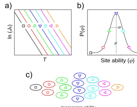
Figure 1. Principles of the multiple-component stochastic model.

Each symbol represents a subpopulation approximated by a single-component system, as shown in (a), with gradient−dln(Js,i)/dT= λand interceptϕ(proxy for nucleating efficiency). The probabil-ity of occurrence for each component, characterised byϕ, is deter-mined using a statistical distribution, as depicted in (b), with a mean

µand standard deviationσ. Applying this probability to a popula-tion of droplets results in an ensemble of droplets exhibiting a range of nucleating efficiencies as in (c).

weighted using a PDF to calculate a probability of occur-renceP (ϕi). Thus, the number of droplets in each

subpopu-lation isnliquid,i=N×P (ϕi), whereN is the total number

of droplets in the simulation. Although there is evidence for multiple components, the distribution of such components is not currently known and difficult to infer. Therefore, for simplicity, a Gaussian distribution was used following previ-ous studies (Niedermeier et al., 2010; Broadley et al., 2012; Wright and Petters, 2013), characterised by a mean µ and standard deviationσ (see Fig. 1). The MCSM can now be defined by summing the number of droplets frozen in each subpopulation for a given time increment:

Nfrozen=

n

X

i=1

nliquid,i 1−exp(−Js,i(T )·Ai·δt )

. (3)

2 Fig. 2

241 242 243 244 245 246

0.0 0.2 0.4 0.6 0.8 1.0

T

/ K





uniform

Figure 2. Illustration of how the systematic shift in temperature

(β)observed for a change in cooling rate is independent of the variability in ice nucleating ability. f (T ) curves shown are for a uniform (σ=0.01) and diverse (σ=20) INP population where

λ=2 K−1, and cooled at constant rates of 1 K min−1(solid line) and 10 K min−1(dashed line).βcorresponds to the shift in temper-ature (K) observed when 50 % of the droplets have frozen.

3 Deriving a new immersion mode framework 3.1 Cooling-rate dependence

In these simulations we look at the sensitivity of the MCSM to changes in cooling rate. The aim is to identify the vari-ables that control the cooling-rate dependent behaviour of a population of droplets. On inspection of Eq. (3) it is evident that for a constant finite negative incrementδT, an increase in cooling rate results in a similar decrease in timeδt, and there-fore a decrease in the probability of a freezing event occur-ring betweenT andT+δT. This is manifested in the number of droplets freezing perδT and results in the entire cumula-tive fraction frozen curve shifting to lower temperatures. This is demonstrated in Fig. 2, with two simulated populations of droplets: one with a uniform INP distribution (a single value of ϕi)and the other with a diverse INP distribution (broad

range of ϕi). Both populations have λ=2 K−1 whereλ is

defined as −dln(Js,i)/dT (i.e. the temperature dependence

of the nucleation-rate coefficient for each component). The simulated droplets were cooled at 1 and 10 K min−1. Figure 2 illustrates how the shift in temperature (β)for a change in cooling rate is independent of the distribution ofϕi. The

in-dependence ofβto the distribution ofϕi has been further

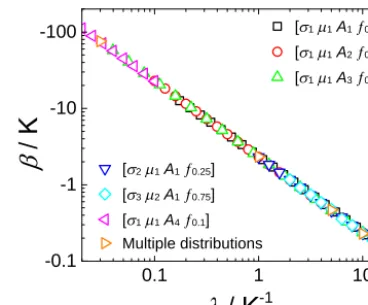
in-vestigated using a series of droplet cooling simulations where all the free variables in the MCSM were allowed to vary be-tween runs, with the corresponding values shown in Table 1. The results from these simulations, shown in Fig. 3, suggest that the only characteristic of the INP population required to quantify its cooling-rate dependence is λ. This is a similar conclusion to Broadley et al. (2012) and Wright and Petters (2013).

3 Fig. 3

0.1 1 10

-0.1 -1 -10 -100

[21A10.25] [32A10.75] [11A40.1] Multiple distributions



[11A10.5] [11A20.5] [11A30.25]

Figure 3. A direct relationship betweenλ(−dln(Js,i)/dT) andβ

(the shift in freezing temperature upon a factor of 10 change in cooling rate) is observed for all droplet cooling simulations. For each set of runsλwas systematically increased whilst the following variables were set: mean (µ) and standard deviation (σ )of the PDF, surface area of particle per droplet (A), and the fraction at which the change in temperature was calculated (f). More information can be found in Table 1.

This result can be understood by rearranging Eq. (1) to describe the change in temperature required to attain a spe-cific cumulative frozen fraction for a given change in cool-ing rate (see Supplement for the full derivation). For a given population of droplets containing an immersed INP charac-terised by the functionJs(T ), the total fraction of droplets frozenf (nr)=nfrozen/Nliquidupon cooling fromT0toTnr in nrsteps, whereNliquidis the number of droplets atT0, can be described as:

f (nr)=1− nr

Y

k=0

(exp−Js(Tk)·A·δt )=

1−exp − nr

X

k=0

Js(Tk)·A·δt

!

, (4)

wherenr denotes the total number of model steps using a

cooling rater, andδt is the time between stepskandk+1. As in Eq. (1) the exponential term essentially describes the cumulative probability of a freezing event not occurring innr

time steps, and can be expanded so thatJs(Tk)=Js(T0)×

(exp(−λδT ))k. By substituting Eq. (2) into Eq. (4) we can explicitly represent the nucleation-rate coefficient:

f (nr)=1−exp −A·δt·Js(T0)

nr

X

k=0

(exp(−λδT ))k

!

. (5)

Table 1. The range of MCSM variables used for droplet cooling simulations in Fig. 3:λis−dln(Js,i)/dT;µandσare the mean and standard

deviation of the PDF used to constrain the occurrence of each component with “formula” referring toµ=240λ+14.8; surface area of immersed INP per dropletA; and the fractionf at which the change in temperature (1T =(fr1)−T (fr2)) for a change in cooling rateris

calculated. All simulations were performed at cooling rates of 1 and 10 K min−1.

Gradientλ/K−1 PDF meanµ PDF widthσ Surface areaA Fractionf

0.2≤λ≤14 formula 1 1×10−7cm2 0.5 0.1≤λ≤16 formula 0.1 5×10−7cm2 0.5 0.04≤λ≤10 formula 1 10×10−7cm2 0.25 1≤λ≤16 formula 5 1×10−7cm2 0.25 2≤λ≤16 formula+10 10 1×10−7cm2 0.75 0.02≤λ≤0.1 formula 1 1×10−7cm2 0.1 0.03 µ1=9,µ2=12 σ1=0.1,σ2=2 1×10−7cm2 0.5

1.0 µ1=255,µ2=265 σ1=1,σ2=2 1×10−7cm2 0.5

5.0 µ1=1255,µ2=1260 σ1=1,σ2=5 1×10−7cm2 0.5

10.0 µ1=2455,µ2=2465, σ1=1,σ2=1, 1×10−7cm2 0.5

µ3=2460 σ3=5

frozen is reached:

Tf (n)=nrδT = (6)

ln

1− _−ln

(1−f (nr))·(1−exp(−λδT ))

A·δt·Js(T0)

₁

−λ−1,

whereδT is the change in temperature between stepskand

k+1. A change in cooling rate from r1 tor2 results in a change in the number of steps1nr to reach fractionf where

f =fn,r1=fn,r2 and therefore a change1Tf:

1Tf =nr2δT−nr1δT =ln

_C·A·δt

r2·Js(T0)

C·A·δtr1·Js(T0)

· 1 −λ, (7)

whereδT is constant for both cases,δt is dependent on the cooling rate, andC= −ln(1−f )×(1−exp(−λδT )). Can-celling terms in Eq. (7) and substituting r1=δT /δtr1 and

r2=δT /δtr2 provides a formula for the change in temper-ature,βcool, observed at a specific fraction frozen for a given change in cooling rate:

1Tf =βcool= 1

λln

_r 1

r2

. (8)

Equation (8) is consistent with the results shown in Figs. 2 and 3; i.e. the systematic shift in cumulative fraction frozen for a change in cooling rate is only dependent on λ. If we assume that all components in a diverse species are char-acterised by a single value of λthis also holds true. Using observations by Vali and Stansbury (1966), Vali (1994) em-pirically found a similar relationship where βcool=0.66× log₁₀(|_r|₎. In our independently derived expression, we take the additional step of linking β toλ, which offers a phys-ical insight to the properties of a particular ice nucleating material; i.e. the empirical relationship from Vali (1994), above, relates to the gradient of the species −dln(Js,i)/dT

so that the distilled water droplets used in the study by Vali and Stansbury (1966) are characterised by the gradient

λ=3.5 K−1.

3.2 Residence-time dependence

In addition to droplet freezing experiments where droplets are cooled at some rate, other experiments (e.g. those using continuous flow diffusion chambers) involve exposing parti-cles to a constant temperature for a defined period of time. In this section we show how measurements made with different residence times under isothermal conditions in such instru-ments can be reconciled by extending theλ-based formula presented in the previous section. Usingr=δT /t, the rela-tive change in cooling rate described by ln(r1/r2) can also be expressed as a relative change in time ln(t2/t1):

βiso= 1

λln

t2

t1

, (9)

whereβisois the shift in temperature required to produce the same frozen fraction in two isothermal experiments with du-ration times oft1andt2.

3.3 σTfreezein freeze–thaw experiments

In freeze–thaw experiments, single or populations of droplets are subjected to repeated cycles of freezing and thawing (Vali and Stansbury, 1966; Durant and Shaw, 2005; Vali, 2008; Fornea et al., 2009; Wright et al., 2013). For each cycle the freezing temperature Tfreeze is determined, and used to in-fer the stochastic nature of the tested material. A freeze– thaw experiment can be simulated when it is realised that one droplet being frozenntimes at a cooling rateris equiv-alent ton identical droplets being frozen a single time at a rater. A single-component system whereϕ equals the me-dianTfreezeprovides a population of identical droplets, which can be used with the MCSM to simulate a single cooling ex-periment. Applying a prescribedndroplets to the resulting

values from n freeze–thaw cycles, and therefore the stan-dard deviation inTfreezecan be determined, hereafter named

σTfreeze (after Wright and Petters, 2013). A series of simu-lations were performed using the MCSM where the median

Tfreezeandλwere varied. A direct relationship betweenλand

σTfreezewas found and is described as:

σTfreeze= 1.2691

λ . (10)

In a single-component system a variation in cooling rate will only result in a change to the median freezing temperature (byβK), thereforeσTfreeze is also independent of the freeze– thaw experiment cooling rate. Equation (10) bears a signifi-cant resemblance to the relationship presented by Wright and Petters (2013):σTfreeze=1.21×λ

−1.05_.

3.4 Reconciling droplet freezing data from different instruments and on different timescales

Since nucleation is a stochastic process, differences in ex-perimental timescale and exex-perimental technique need to be reconciled. First we reconcile isothermal data with cooling experiments so they are consistent with each other. This can be achieved by equating the simulated fraction frozen using both methods at the same temperature:

fiso(T )=fcool(T ) , (11)

where “cool” denotes a cooling experiment simulation from

T0=273.15 K and “iso” an isothermal experiment simu-lation at a temperature T. The fraction frozen during an isothermal simulation is calculated similarly to a cooling ex-periment except the temperature remains constant through-out; thus, we can use Eq. (4) to describe an isothermal simu-lation:

fiso(T )=1−

niso Y

k=0

exp(−Js(Tk)·A·δtiso), (12)

Js(Tk)=Js(T ) , (13)

therefore,

fiso(T )=1−exp(−Js(T )·A·δtiso·niso) , (14) where niso is the total number of time steps,δtiso, for the isothermal simulation. Substituting Eqs. (14) and (4) into Eq. (11) yields:

1−exp −Js Tncool

·A·δtiso·niso

=

1−exp − ncool X

k=0

Js(Tk)·A·δtcool !

, (15)

which, when simplified gives the total time (ttotal)required for an isothermal experiment to reach the same fraction as a cooling experiment at temperatureT:

δtiso·niso=ttotal,iso Tn_cool

= 1

Js(Tncool) n_cool X

k=0

Js(Tk) δtcool. (16)

Substituting in Eq. (2), after expanding as in Sect. 3.1, and rearranging yields:

ttotal,iso Tncool ₌

δtcool

ncool X

k=0

(exp(λδT ))k. (17)

Using a summation of series the summation term is removed and the formula can be simplified:

ttotal,iso Tncool

= δtcool 1−exp(λ·δTcool)

. (18)

A Taylor expansion of exp(λ×δTcool) will result in the series 1+λδTcool−1/2(λδTcool)2+1/6(λδTcool)3. . .. When

λδTcool1/2(λδTcool)2,exp(λδTcool)∼=1+λδTcool. This is satisfied when the simulation temperature step

λδTcool1. We can then simplify this formula using

rcool=δTcool/δtcool, wherercool>0, so that:

ttotal,iso Tncool

= δtcool

λ·rcool·δtcool

= 1

λ·rcool

. (19)

Assuming that the nucleation-rate coefficient of a species is approximated by the functional form in Eq. (2), this gives the time required for an isothermal experiment to reach the same frozen fraction as in a cooling-rate experiment at a specific temperature. Againλ(the gradient of the nucleation-rate co-efficient) controls the time-dependent nature of immersion mode droplet freezing.

Now that isothermal and cooling experiments are recon-cilable, artefacts introduced through the time-dependent be-haviour of an INP in an experiment can be normalised to a standard raterstandard, for which we have chosen 1 K min−1. For cooling experiments, replacingr1in Eq. (8) withrstandard andr2with the experimental cooling rater, in K min−1, gives

βas a function of the absolute cooling rate:

β (r)=1T =1

λln

₁ |_r|

. (20)

For isothermal experiments, replacingrcoolwithrstandard in Eq. (19) gives the time required for an isothermal experiment to be comparable to a normalised cooling experiment. Sub-stitutingt1in Eq. (9) withttotalin Eq. (19), andt2with the experimental residence timet, in seconds, givesβas a func-tion of residence time:

β (t )=1T =1

λln

_λ·t 60

. (21)

Experimental data can then be modified and normalised us-ingT0=Texperiment−β, whereT0is the normalised temper-ature, andTexperimentthe temperature of the experiment data point.

3.5 Incorporating the FROST framework into a singular model

As discussed in Sect. 1.1.2, the singular freezing model is well suited to describing the interparticle variability of ice nucleating ability, but it does not describe the time-dependent nature of nucleation. The probability of a droplet freezing is often described by the active site density (Demott, 1995),

ns(T ), (also called the ice active surface site density; Con-nolly et al., 2009; Murray et al., 2012; Hoose and Mohler, 2012) which describes the cumulative number of freezing events that can occur betweenT0andT:

f (T )=1−exp(−ns(T )·A) . (22)

Vali refers to a similar quantity (expressed per volume rather than surface area) as the cumulative nucleus spectrum (Vali and Stansbury, 1966; Vali, 1971, 2014). By rearranging Eq. (22) it can be seen thatns(T )(in cm−2)is directly re-lated to the cumulative fraction frozen:

ns(T )= −

ln(1−f (T ))

A . (23)

It is therefore apparent that a systematic shift in the cumula-tive fraction frozen, caused by a change in the cooling rate or residence time, results in a systematic shift inns(T )so that, upon incorporating Eq. (20) into Eq. (23), we find that for a specific cooling rater(wherer> 0),

f (T , r)=1−exp

−ns

T−ln(|r|) −λ

·A

. (24)

The differentiation ofnswith respect toT results in the func-tionk(T )that can be used to calculate the change in the frac-tion frozen occurring upon a lowering ofT:

1f (T , r)=1−exp

−k

T−ln(|r|) −λ

·A·1T

, (25)

where k(T ) is in units per square centimetre per kelvin (cm−2K−1). Equations (24) and (25) are consistent with the empirical “modified singular” equation presented by Vali (1994), but here we have linked the stochastic term to the temperature dependence of the nucleation-rate coefficient.

Similar equations can also be defined for isothermal ex-periments by incorporating Eq. (21) into Eq. (22) so that at a specific temperature,Tiso, and residence time in seconds,t,

f (T , t )=1−exp

−ns

T −1

λln

_λ·t 60

·A

. (26)

Again, upon differentiation we obtain an equation for the change in fraction frozen upon a change in residence time fromt tot+1t:

1f (T , t )=1−exp

−k

T−1 λln

_λ·t

60

·A· 1 −λ·t1t

, (27) where1t/(−λ×t )has replaced1T through the incorpo-ration of Eq. (19) into1T = −r/ 60×1t;ris in kelvin per minute (K min−1) and1tin seconds.

4 Testing the FROST framework

In the previous section we presented the FROST framework which is a new immersion mode ice nucleation framework designed to represent both the interparticle variability of ice nucleating efficiencies and the stochastic (time-dependent) nature of nucleation. In this section the FROST framework will be tested using a combination of original experimental droplet freezing data and literature data for atmospherically relevant INPs obtained from a range of methods and instru-ments. The terminology here follows that of Vali (2014) in that experimental data are presented using the freezing rate

R. A normalisation ofR to surface areaAis used to com-ment on the relationship betweenRand the nucleation-rate coefficientJs, as well as whether the species behaves as a single- or multiple-component species.

4.1 Kaolinite data (KGa-1b) from two cold-stage instruments

In this example data from droplet freezing experiments on two cold-stage instruments, with a range of cooling rates, are combined to test the capability of the FROST framework. The first data set, referred to as PICOLITRE, is taken from Murray et al. (2011), hereafter referred to as M11. In their ex-periments micron-sized droplets containing known amounts of kaolinite (KGa-1b, Clay Mineral Society) mineral dust and supported on a hydrophobic surface, were cooled at con-stant rates on a cold stage coupled with an optical micro-scope. Each experiment was characterised by a specific cool-ing rate and weight fraction of mineral per droplet. For this study four data sets are used (experiments vii, viii, ix and xi in M11) corresponding to cooling rates (weight fractions) of 5.4 (0.0034), 9.6 (0.01), 0.8 (0.01) and 5.1 (0.01) K min−1, respectively. For the second experimental data set, referred to as MICROLITRE, a different cold-stage instrument was used, which has been described previously (O’Sullivan et al., 2014; Whale et al., 2014). In this experiment∼40 droplets of 1 µL volume containing known amounts of the same kaoli-nite sample as M11 (KGa-1b) were held on a hydropho-bic surface and cooled at constant rates with freezing events recorded optically. Four experiments were performed at cool-ing rates of 0.1, 0.2, 0.5, and 1.0 K min−1. All experiments were performed with a weight fraction of 0.01, correspond-ing to a surface area of 1.178±0.3 cm2per droplet calculated using a specific surface area of 11.8±0.8 m2g−1 _(M11). The uncertainty in surface area per droplet primarily arises from uncertainty in specific surface area measurements and droplet volume. The temperature uncertainty, arising from the temperature probe and observed range in melting temper-atures, has been estimated by Whale et al. (2014) as±0.4 K. Freezing data are limited toT > 252.65 K, below which the substrate is observed to influence freezing behaviour.

Fig. 4

238 243 248 253 258

-10 -5 0 5 10 15

PICOLITRE 0.8 K min-1

5.1 K min-1

5.4 K min-1

9.6 K min-1

MICROLITRE 0.1 K min-1

0.2 K min-1

0.5 K min-1

1.0 K min-1

T

/ K

a)

0 3 6 9 12 15

-3 -2 -1 0



Tiso= 255.15 K

b)

Isothermal experimental data Expected decay atTiso0.4 K

Time / minutes

1 2 5 10 15

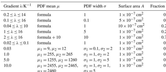
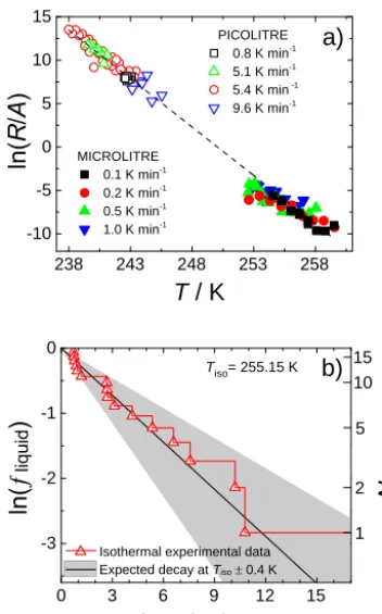
Figure 4. Droplet freezing data for kaolinite (KGa-1b). (a) shows

freezing rates normalised to surface area,R/A, against temperature determined from droplet freezing experiments with a range of cool-ing rates. Open symbols represent PICOLITRE experiments from Murray et al. (2011) and closed symbols represent MICROLITRE experiments. The black dashed line shows a linear fit to all data (ln(R/A)= −1.12T +280). Temperature uncertainty for the MI-CROLITRE data (not shown) is estimated at ±0.4 K, and un-certainty in R/A (not shown) is estimated at −17 and +25 %.

(b) shows the exponential decay of liquid droplets during an

isother-mal experiment at 255.15 K together with a modelled experiment at the same temperature using the linear fit to all data in (a). The grey area follows the experimental uncertainty inT around the modelled isothermal. The experiment duration was 17 min, at which point one droplet remained unfrozen.

Fig. 4a. The larger droplets in the new MICROLITRE ex-periment contain significantly greater INP surface area per droplet than the PICOLITRE experiment, which increases the probability of freezing, resulting in higher freezing tem-peratures. The freezing rates plotted in Fig. 4a are derived using Eq. (1), hence the assumption in performing this anal-ysis is that the species has a uniform INP distribution and be-haves as a single-component system, and thus the normalised freezing rateR/Ais directly equivalent to the nucleation rate

Js,i. However, at this stage we do not know if this assumption

is valid.

In a single-component system the gradient−dln(R/A)/dT, named ω following Vali (2014), is equal to λ (recall that

λ= −dln(Js,i)/dT ). If it were a multiple-component system

then the slopeωwill be smaller thanλbecause an inappro-priate model was used (i.e.ωis a lower limit toλ). For a set of data obtained at a single cooling rate it is impossible to say if it is a single- or multiple-component sample, further tests are required. M11 did this by performing isothermal ex-periments in addition to exex-periments at various cooling rates and showed that the values ofR/Aderived from both exper-iment styles were consistent and concluded that nucleation by kaolinite KGa-1b behaved as a single-component sys-tem below 246 K and thereforeR/A=Js,i.We expand on

this earlier analysis with additional data for kaolinite KGa-1b at warmer temperatures and place it in the context of the FROST framework. To test whether the MICROLITRE data set is also consistent with a single-component system we per-formed an isothermal experiment, in addition to the experi-ments at various cooling rates.

The isothermal experiment, shown in Fig. 4b, was per-formed at 255.15 K with droplets containing a weight frac-tion 0.01 of KGa-1b particles. We have plotted the de-cay of liquid droplets expected based on a value of Js,i

at 255.15±0.4 K determined from the linear fit to ln(R/A)

in Fig. 4a. The expected exponential decay matches the measured decay; this is consistent with a uniform species, and thus a single-component system. The derivedR/A val-ues from experiments at cooling rates ranging from 0.1 to 1.0 K min−1are shown in Fig. 4a and also show consistency with this system.

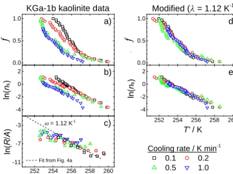
In Fig. 5 we place the data from the cooling experiments in the context of FROST. If the INP species can be characterised with a singleλthen the application of Eq. (20) will modify each data point byT0=Texperiment−β (r). With the correct value ofλin the FROST framework, the data will converge onto the curve of a 1 K min−1 _{cooling experiment for the} species tested. Figure 5a, b, and c show the fraction frozen

f (T ), ns(T ) values, and R/A(T ) values from Fig. 4a, re-spectively. Thens(T )values, derived using Eq. (23), depend on the cooling rate, with over a factor of 5 shift on changing the cooling rate by a factor of 10. On applying FROST with

λ=1.12 K−1(thus assumingλ=ω from Fig. 4a) both the modifiedf (T0)andns(T0)data converge (Fig. 5d and e, re-spectively). This additionally supports the claim that kaolin-ite KGa-1b is well represented by a single-component system (R/A=Js,i).

An interesting and potentially significant issue is raised by this study of nucleation by kaolinite as the linear fit to the two independent data sets in Fig. 4a is made over 20 K which is at odds with CNT. CNT predicts curvature in lnJs versus

5 Fig. 5

0.0 0.5 1.0



Cooling rate / K min-1

0.1 0.2

0.5 1.0

T/ K

Modified (= 1.12 K-1 ) KGa-1b kaolinite data

a)

b)

c)

d)



e) 0.0

0.5 1.0

T'/ K

-4 -2 0 2

252 254 256 258 260 -4

-2 0 2

252 254 256 258 260 -11

-7 -3

Fit from Fig. 4a = 1.12 K-1

Figure 5. The freezing of droplets containing kaolinite (KGa-1b) in

cooling experiments (MICROLITRE). (a) Rawf (T )data, (b) de-rivedR/A(T ), (c)ns(T )values, (d) the corresponding normalised f (T0)data, and (e) normalisedns(T0). Data were normalised

us-ing the value ofλdetermined directly from the linear fit to ln(R/A) againstT in Fig. 4a and reproduced in (c). Temperature andR/A

uncertainty is as in Fig. 4. Uncertainty inns(not shown) is estimated

as±20 %.

to understand this potentially important finding, but is be-yond the focus of this paper.

While nucleation by this kaolinite sample can be treated as a single component, this does not necessarily mean that this sample is uniform (i.e. there is no interparticle variabil-ity) because there are many particles per droplet in the ex-periment. It is possible, but unlikely, that droplets contain a distribution of particles with diverse ice nucleating abili-ties, but where freezing in all droplets happens to be con-trolled by particles with similar ice nucleating activity. This is very unlikely given that the number of kaolinite particles in the PICOLITRE experiments ranges from just a few tens to tens of thousands and all produce consistent values ofJs (M11). In contrast, the Fluka kaolinite sample used by Welti et al. (2012), which is known to contain particles of very effi-cient feldspar (Atkinson et al., 2013), is a diverse species (as will be demonstrated in Sect. 4.3).

In summary, kaolinite KGa-1b from the clay mineral so-ciety is an example of a material which most likely has ap-proximately uniform ice nucleating properties and can be de-scribed with a single-component stochastic model.

6 Fig. 6

0.0 0.5 1.0

Cooling rate / K min-1

0.2 (2) 0.4 (2) 1.0 (5) 2.0 (2) Modified (= 3.14 K-1

) K-feldspar data

a)

 

T/ K

T'/ K

0.0 0.5

1.0 _d)

260 261 262 263 264 265 -4

-2 0 2

= 0.85 K-1

= 0.9 K-1 c)

260 261 262 263 264 265 0

2 4 6

Fit from Atkinson (2013)

e)

0 2 4

6 _b)

Figure 6. The freezing of droplets containing K-feldspar for a range

of cooling rates. Layout as in Fig. 5. Brackets beside the cool-ing rates indicate the number of experiments performed and sub-sequently combined. Linear fits to derived ln(R/A) values for runs at 0.2 and 2.0 K min−1 are shown as solid lines in (c) resulting inω=0.85 and 0.9 K−1, respectively. Modifiedns(T0) data were

minimised in order to determine a value ofλthat best describes the cooling-rate dependence, resulting inλ=3.4 K−1. In this example

ω6=λsuggesting that K-feldspar is a diverse INP species and be-haves as a multiple-component system. The dashed line in (e) is a fit to K-feldspar experimental data taken from Atkinson et al. (2013). Temperature uncertainty is as in Fig. 4, and uncertainty inns and R/A(not shown) is estimated as±25 %.

4.2 K-feldspar data from a cold-stage instrument In this example we investigate and determine the cooling-rate dependence of K-feldspar using the microlitre droplet instrument as in the previous example. K-feldspar was re-cently shown to be the most important mineral component of desert dusts for ice nucleation (Atkinson et al., 2013). In these experiments∼40 droplets of 1 µL volume were cooled at constant rates of 0.2, 0.4, 1.0 and 2.0 K min−1 on a hy-drophobic surface. Each droplet contained a weight frac-tion 0.001 of K-feldspar, corresponding to a surface area of 1.85×10−2±0.004 cm2calculated using a specific surface area of 1.86 m2g−1(Whale et al., 2014).

Similar to the previous example, Fig. 6a, b, and c show the experimental fraction frozen data f (T ), and derived

ns(T ) and R/A(T ) values, respectively. For the 0.2, 0.4 and 2.0 K min−1_{curves two separate experiments were} per-formed and for the 1.0 K min−1_{curve five experiments were} performed. A systematic shift inf (T )outside of instrumen-tal error (±0.4 K) can be seen for the experiments at 0.2 and 2 K min−1, which indicates that there is a cooling-rate depen-dence for nucleation by K-feldspar.

Fig. 6c. If K-feldspar behaved as a single-component system then the two data sets would fall onto the same line, as they do for kaolinite in Fig. 4a. However, they do not fall on the same line; theR/Avalues are significantly different between the two cooling rates, hence this suggests that K-feldspar is a diverse species and requires a multiple-component model to describe its freezing behaviour. In this case Eq. (1) should not be used to derive values of nucleation-rate coefficients sinceR/A6=Js,i.

As stated in the previous section, with the correct value of λin the FROST framework, the modified data will con-verge onto a single curve. Therefore, in order to determine the value of λ,a procedure was followed where λ was it-eratively varied until ns(T0), whereT0=Texperiment−β (r), converged onto a single curve (using Eq. 20). The best fit was determined by minimisation of the root-mean-square error (RMSE) between the data and a linear fit to ln(ns)for data where Texperiment≤262.65 K (−10.5◦C); this temperature was chosen to limit effects from anomalous high-temperature freezing events that are statistically unrepresentative of the INP species. This fitting procedure, with a RMSE value of 0.009, resulted inλ=3.4 K−1and is shown in Fig. 6e. This value is significantly steeper than the gradientsωin Fig. 6c (0.85 and 0.9 K−1). Recall that for kaolinite, the gradientω

was used to normalise the ns values in Fig. 5e which sug-gests that kaolinite is a uniform species. For K-feldspar the fact that ω6=λ (where λ= −dln(Js,i)/dT ) shows that

K-feldspar exhibits a diverse nucleating ability across the pop-ulation.

Figure 6e also includes the fit to K-feldspar data presented in Atkinson et al. (2013). In their study the surface area of K-feldspar per droplet was increased by 2 orders of magni-tude to examine the dependence of freezing rate on surface area and all experiments were performed at a cooling rate of 1 K min−1. The parameterisation from Atkinson et al. (2013), based on data with variable surface areas, is in good agree-ment with data from the present study.

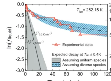
An isothermal experiment was also performed at

Tiso=262.15 K with 20 droplets (28 froze during cooling to

Tiso)containing a weight fraction 0.001 of K-feldspar (see Fig. 7). For a uniform species the decay of liquid droplets over time will be exponential (as was the case for kaolinite KGa-1b in Fig. 4b), whereas a diverse species will result in a non-exponential decay. Inspection of the data in Fig. 7 shows that the decay of liquid droplets was not exponential, again consistent with a diverse population of INPs. To highlight this, we have plotted the decay expected from the two limit-ing values ofR/Afrom Fig. 6c at 262.15 K. The simulated decays, assuming a single-component system, clearly over-predict the rate of decay. We also simulate what we would expect for a diverse population where we use the MCSM to produce the expected decay of droplets. The MCSM was ini-tially used as a fitting tool to obtain a distribution that best reproduced the entire normalised f (T0)data set in Fig. 6d, using the minimised value λ=3.4 K−1 determined

previ-7 Fig. 7

0 20 40 60 80 100 120

-3.0 -2.5 -2.0 -1.5 -1.0 -0.5 0.0

Tiso= 262.15 K

Experimental data

Expected decay atTiso0.4K

Assuming uniform species Assuming diverse species

1 2 5 10 1520



Time / minutes

Js(T0.2 Kmin-1)

Js(T2 Kmin-1)

Figure 7. Decay of liquid droplets containing K-feldspar in an

isothermal experiment atTiso=262.15 K, and simulated

experi-ments assuming a uniform and diverse distribution. For the uniform distributionJs(Tiso)values were taken from Fig. 6a (thus assuming

a single-component system whereJs=R/A) and used with Eq. (1),

resulting in a decay bounded by the range ofR/Abetween the two cooling rates of 0.2 and 2.0 K min−1. For the diverse simulation the MCSM was used with parameters determined through fitting to the normalised K-feldspar data set in Fig. 6:µ=890.5,σ=3.8 (see Fig. 1), andλ=3.4 K−1(determined in Fig. 6). The shaded regions follow the instrument-based error of±0.4 K aroundTiso. The

trian-gular symbols indicate when freezing events occurred throughout the 120 min duration of the experiment.

ously. This distribution (µ=890.5,σ =3.8) was then used to simulate an isothermal experiment. These simulations in-cluded the initial cooling period required to reach the su-percooled temperature. There is clear consistency between the diverse simulation and the experimental data. This again shows strong evidence that the K-feldspar sample used is a diverse species and would require a multiple-component sys-tem to describe its freezing behaviour.

This example is important as it illustrates that for a diverse INP species with multiple active components, the observed gradientωof the derivedR/A(T )values from a single ex-periment does not characterise its stochastic behaviour. For these species a series of experiments at different cooling rates or residence times must be performed in order to determine the value ofλthat can be used to characterise its stochastic behaviour.

4.3 Mineral dust freezing experiments from the Zurich Ice Nucleation Chamber (ZINC)

8 Fig. 8 236 238 240 242 15

19 23 0.0 0.5 1.0

~Residence time / s

1 2 3 6 9 10 21

Modified (= 2.19 K-1 ) Fluka kaolinite data

a)

b)

c)

d)

e)



T/ K

T'/ K



0.0 0.5 1.0

15 18 21

236 238 240 242 15

18 21

0.2 K-1

1.2 K-1

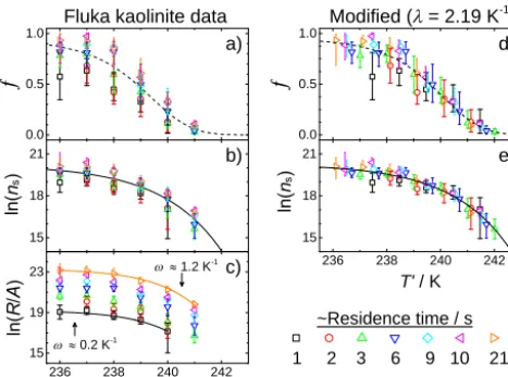
Figure 8. The freezing of droplets containing size-selected 400 nm

kaolinite (Fluka) particles in a CFDC instrument from Welti et al. (2012). Layout as in Fig. 5. Residence times at constant tem-perature ranged from 1.11 to 21.4 s at temtem-peratures from 236 to 241 K. R/A(T ) values, shown in (c), do not fall onto a single line and exhibit a consistent separation with increasing residence time. Modifiedns(T0)data were minimised in order to determine

a value ofλ that best describes the time dependence, resulting in

λ=2.19 K−1. The minimisedns(T0)values and corresponding fit

(RMSE=0.047) are shown in (e). For comparison the same fit-ting function was applied to the rawns(T )data (RMSE=0.076)

and is shown in (b). These two functions were used to reproduce a 1 K min−1cooling experiment and are shown as dashed lines in (a) and (d). Error bars are reproduced from Welti et al. (2012).

supercooled droplets, and passed the droplets into the ZINC instrument. Within ZINC the droplets experienced isother-mal conditions and the frozen fraction was determined using a depolarisation detector. Variable flow rates and a series of detection points provide a range of residence times, and by performing experiments at several temperature W12 built up

f (T )curves for a range of residence times. For this study we use the data for 400 nm particles. The data are shown in Fig. 8a along with derivedns(T )andR/A(T )values in b and c, respectively. Similar to the K-feldspar data the R/A(T )

values for the mineral dust do not fall onto a single line and show a separation between residence times consistent with a multiple-component system. Therefore, in order to deter-mine the value ofλthat describes the residence-time depen-dence, the same procedure was followed as in Sect. 4.2 for K-feldspar.

Each data point represents a single isothermal experiment with a single residence time,t. Hence, Eq. (21) can be used to modify each data point withT0=Texperiment−β (t ), assum-ing that the species can be characterised by a sassum-ingle value forλ. Using derivedns(T )values, with INP surface area per droplet calculated assuming a spherical particle 400 nm in diameter as per the experiment,λwas systematically varied until the ns(T0)values converged onto a single line, again

described by an exponential fit to ln(ns). This resulted in

λ=2.19 K−1 _{with a ln(n}

s) RMSE of 0.047, and is shown in Fig. 8e. For comparison, an exponential fit describing the rawns(T ) data resulted in a RMSE of 0.076. The two ex-ponential fits were used to reproduce the expected fraction frozen data for a 1 K min−1cooling experiment, and are plot-ted along with the observed and normalised fraction frozen data set in Fig. 8a and d, respectively. The range ofω de-termined from the ln(R/A)fits in Fig. 8c was estimated as 1.2 K−1at 240.5 K and 0.2 K−1at 237.5 K. These values are lower than the minimised value ofλ(2.19 K−1)suggesting that the mineral dust sample used in the W12 study is a di-verse species and requires a multiple-component model to describe its freezing behaviour, which agrees with the con-clusions of W12.

Similar to the kaolinite and K-feldspar examples the deter-mined value ofλwas used to reproduce the expected decay of liquid droplets over time. With CFDC (Continuous Flow Diffusion Chamber) instruments the cooling from ambient temperature to the experimental temperature is very rapid and therefore the distribution of INP efficiency per droplet can be assumed to be represented by the function ofns(T0) determined in Fig. 8e. To calculate the expected decay of liq-uid droplets with time Eq. (26) was used with the value of

λ(2.19 K−1) determined previously. The experimental data, along with the expected decay, are shown in Fig. 9. It can be seen that at high temperatures (241–239 K) the FROST framework is able to reproduce the experimental decay very well. However, at lower temperatures (238–236 K) there are large differences, especially for longer residence times. The reported errors bars are large for the lowest temperature data and suggest an increasing uncertainty with decreasing tem-perature. Also the fraction of droplets frozen is expected to increase with decreasing temperature as stated by W12. This suggests a potential experimental issue, which would explain the discrepancies.

Here the FROST framework has been used to both nor-malise isothermal experiments performed over a range of res-idence times, and determine a value ofλ that can be used to potentially describe the cooling-rate and time-dependent behaviour of this mineral dust in simulations. This example additionally highlights the necessity to use relatively pure samples in order to limit uncertainties due to multiple INP species.

4.4 Volcanic ash from ZINC and AIDA

9 Fig. 9

0 2 4 6 8 10 12 14 16 18 20 22

-9 -6 -2 -1 0

Tiso/ K

241 240 239 238 237 236

(



Time / s

Figure 9. Experimental fraction unfrozen data for droplets

contain-ing Fluka kaolinite (symbols) in Fig. 8a (Welti et al., 2012) plotted as a function of time and temperature. We also plot the expected decay of liquid droplets with time determined using Eq. (26) with the function ofns(T0)in Fig. 8e andλ=2.19 K−1. The expected

decay at each temperature is shown as a dashed line.

chamber (Hoyle et al., 2011; hereafter H11). The ZINC in-strument, as described in the previous section, was used to determine the total fraction of droplets frozen over a range of temperatures (230≤T ≤247 K) with a residence time of 12 s at each temperature; each supercooled droplet contained a single immersed particle, which ranged from∼0.1 to 3 µm in diameter,D. The 84 m3AIDA cloud chamber is capable of simulating an ascending, cooling air parcel, and is coupled to an array of instruments, which were used to determine the freezing characteristics of the same volcanic ash sample; in this method the dust sample (∼0.1≤D ≤ ∼15 µm) is dis-persed into the cloud chamber prior to expansion.

The ice nucleating efficiencies of the two data sets were compared in Murray et al. (2012) and the subsequentf (T )

andns(T )values are reproduced in Fig. 10a and b, respec-tively. Although the fraction frozen data appear to be con-sistent between studies, once plotted as ns(T ) it is clear that the two data sets, albeit with similar gradients, do not show good agreement even though the same sample was used. Figure 10c shows the surface-area normalised freez-ing rates,R/A(T ), calculated using the temporal conditions of each experiment. For the H11 data the experimental resi-dence time of 12 s was used, and for the S11 a cooling rate of 1.074 K min−1_{was used (determined from the point at which} water saturation was reached, until the elapsed time of the ex-periment had reached 300 s as per Fig. 2 in S11). Due to the non-cumulative nature of the S11f (T )data set a polynomial fit to the data was used to determine the differential fraction frozen required to calculate R/A(T ) values. The two data sets fall onto a single line with a ln(R/A)RMSE of 0.22 and a gradient ω= −dln(R/A)/dT =0.55 K−1. Following the previous two examples,λwas systematically varied until thens(T0)values converged onto a single line described by

Fig. 10 10-4

10-3

10-2

10-1

100

10-4

10-3

10-2

10-1

100

9 11 13 15 17

237 241 245 249

9 11 13 15 17

235 239 243 247 6

8 10 12 14

Data source & instrument Hoyle 2011 (AIDA) Steinke 2011 (ZINC) Modified(= 0.60 K-1) Volcanic ash sample

a)

b)

c)

d)

e)



T/ K



T'/ K

Fit to combined dataset

Fit to combined dataset = 0.55 K-1

Figure 10. Freezing of droplets containing volcanic ash sampled

from the Eyjafjallajökull eruption in 2010. Layout as in Fig. 5. Red circles represent data presented in Hoyle et al. (2011) using the ZINC instrument, and blue squares represent data from Steinke et al. (2011) using the AIDA expansion chamber.ns(T )data in (b)

were reproduced from Murray et al. (2012);f (T )values in (a) were also determined from this data set. A fit to determinedR/Avalues in (c) resulted inω=0.55 K−1. The rawns(T )data were modified

by iteratively decreasingλuntilns(T0)values collapsed on a single

line, resulting inλ=0.60 K−1. The similarity inωandλsuggests that this volcanic ash sample behaves as a single-component sys-tem.

an exponential fit to ln(ns), resulting inλ=0.60 K−1. Apply-ing this value to Eqs. (20) and (21) results inβ(r)= −0.12 K andβ(t )= −3.57 K for the S11 and H11 data sets, respec-tively. Figure 10d and e show the subsequently modified

f (T0)andns(T0)data, respectively. The modified fraction frozen data show a difference between data sets due to the larger surface-area per droplet in the H11 experiments (also evident in Fig. 10b). Thens(T0)data are shown in Fig. 10e, with a linear fit to the combined data set producing a ln(ns) RMSE of 0.25.

Fornea et al. (2009) also performed an immersion mode experiment using a volcanic ash sample from Mount St He-lens. In their experiments single particles with a diameter of 250≤D≤300 µm were immersed within five 2 µL droplets and each subjected to 25 freeze–thaw events on a cold-stage instrument. Additionally, as a means of testing the sensitiv-ity to cooling rate, droplets containing the same volcanic ash sample were subjected to freeze–thaw cycles, but cooled at different rates (1–10 K min−1). The freeze–thaw experiments resulted in an averageσTfreeze of 2.0 K and the variable cool-ing experiments resulted in a shift in the average freezcool-ing temperature by 3.6 K (upon a change from 1 to 10 K min−1)

without any change in σTfreeze. Applying these data to the FROST framework Eqs. (10) and (20) were used to deter-mine λ, resulting in λ=0.635 K−1 andλ=0.640 K−1 for the freeze–thaw and cooling experiments, respectively. The first important point worth noting is that these two values, determined from distinct experimental and analysis meth-ods, show very good agreement. Secondly, a comparison to the values determined for the Eyjafjallajökull ash sample (ω=0.55 K−1andλ=0.60 K−1)shows that there is a strong similarity with regards to the magnitude ofλ. Even though these volcanic ash samples are from different sources these results suggest that they have similar time-dependent prop-erties. These additional results provide evidence that the λ

value determined for the Eyjafjallajökull sample is robust, and therefore supports the conclusion that the Eyjafjalla-jökull ash sample tested is a single-component species.

5 Discussion

5.1 The sensitivity of freezing probability to the time dependence of nucleation

It is apparent that the stochastic behaviour of ice nucleation can be manifested as both a residence-time and cooling-rate dependence. For INP species characterised by a single value of λthis collective time dependence can be reconciled and predicted using the FROST framework. Within this frame-work a change in cooling rate or residence time can be seen as an equivalent shift in temperature along the function de-scribing the nucleation rate. This function is typically expo-nential and therefore can have a significant effect on the re-sulting freezing probability.

A first-order indication of the potential importance of time dependence is shown in Fig. 11 where values of βcooland

βisofor 0.4≥λ≥10 K−1have been plotted. Each point rep-resents the shift of a specific fraction frozen, by a temperature

β K, that results from a fractional change in either cooling rate or residence time for a species with a specific value ofλ

as per Eqs. (8) and (9). This plot shows how materials with a small value ofλ(corresponding to a shallow gradientωin a single-component system) are more sensitive to timescale;

Fig. 11

0.5 0.60.70.80.91 2 3 4 5 6 7 8 0.1

1 10

1 1 1

-1 0.8

0.6



0 K

10 1 0.1

Figure 11. The shift in temperatureβK that will result from a frac-tional change in cooling rate or residence time as a function ofλ. Estimated values include those determined from (i) this study, (ii) Wright et al. (2013) cooling experiments, (iii) Wright et al. (2013) freeze–thaw experiments, (iv) Fornea et al. (2009), (v) Vali (2008), and (vi) Vali and Stansbury (1966). INP samples are colour coded depending on INP type. Blue (solid and dashed) arrows correspond to rain samples (unfiltered and filtered) from the freeze–thaw exper-iments presented in Wright et al. (2013).

with a decreasingλcorresponding to an increasing shift by

βfor the same change in timescale.

The values ofλ from this study and other experimental data sets in the literature (Vali and Stansbury, 1966; Vali, 2008; Fornea et al., 2009; Wright et al., 2013) have been in-cluded in Fig. 11; the values and associated study are addi-tionally shown in Table 2. In each case the FROST frame-work was used to estimateλ from cooling, isothermal and freeze–thaw experiments as per Eqs. (20), (21), and (10). It is clear that atmospherically relevant INPs exhibit a wide range of time-dependent behaviour. INP species that have a value ofλwith a large magnitude (λ> 4 K−1), such as Icemax™, and Arizona Test Dust (ATD), will exhibit very little time de-pendence and would likely be well approximated by a singu-lar freezing model. For those with a small magnitude (espe-ciallyλ< 1 K−1)such as kaolinite KGa-1b and volcanic ash, the significant cooling-rate and residence-time dependence must be taken into account. It is interesting to note that in many previous studies into the role of time dependence (Vali and Stansbury, 1966; Vali, 2008; Welti et al., 2012), which formed the basis of the argument that time dependence is of secondary importance, the materials used have largerλ val-ues and are therefore less sensitive to temporal conditions.

Table 2. Summary ofλvalues from various immersion mode studies determined using the FROST framework.

Study and experimental method Material λ/K−1 Vali and Stansbury (1966) – cooling Distilled water 3.5 Vali (2008) – freeze–thaw Soil

Distilled water

6.3 3.0 Fornea et al. (2009) – freeze–thaw Volcanic ash (Mt St Helens) 0.6 Fornea et al. (2009) – cooling Volcanic ash (Mt St Helens) 0.6 Hoyle et al. (2011) – isothermal

& Steinke et al. (2011) – cooling

Volcanic ash (Eyjafjallajökull) 0.6 Welti et al. (2012) – isothermal Kaolinite Fluka 2.2 Wright et al. (2013) – freeze–thaw Icemax™

ATD

Montmorillonite Kaolinite KGa-2b Flame soot Filtered rain #1 Filtered rain #2 Filtered rain #3 Filtered rain #4 Unfiltered rain #1 Unfiltered rain #2 Unfiltered rain #3

2.9 2.3 0.9 2.2 1.7 1.3 2.0 2.6 1.9 1.6 1.4 1.9 Wright et al. (2013) – cooling Icemax™

ATD

Montmorillonite Kaolinite KGa-2b Flame soot Filtered rain #3 Filtered rain #4 Unfiltered rain #1

N/A∗ 4.4 1.8 1.7 1.4 4.6 4.6 N/A∗ This study – cooling and isothermal Kaolinite KGa-1b

K-feldspar

1.1 3.4

∗_{Due to the experimental scatter in reported data it was not possible to estimateλfor these species.}

experiments by Wright et al. (2013) for kaolinite KGa-2b and Icemax™ are very similar, but the Icemax™ sample nucle-ated ice at much warmer temperatures. More work needs to be done on what factors control the value ofλ.

The finding that ice nucleation by different materials has different sensitivities to time is important because it changes the way we should frame the debate of whether time depen-dence plays an important role in ice nucleation. In the past the question has been whether time dependence is important, but this question should be rephrased to whether a particular INP species has a strong time dependence or not, and at what point this stops having an impact on ice nucleation rates; i.e. is there a limiting value ofλbeyond which the singular freez-ing model is adequate?

5.2 Representing complex INP populations in cloud models

The range in time-dependent behaviour shown for the INP species in Fig. 11 leads to the question of how to best

imple-ment this behaviour for a complex multiple-component INP sample, or population, where each component has a charac-teristic time dependence, within a cloud model.

The time dependence of a population of INPs containing many separate species may be dominated by a single compo-nent, and therefore a single value or temperature-dependent function ofλ. Where distinct components are dominant in different temperature ranges it would be possible to have a temperature-dependent function of λ to reflect the relative dominance of each component. For multiple-species aerosol where no single component is observably dominant, the pop-ulation of particles/droplets would need to be split into sep-arate components and treated as an externally mixed popula-tion.

used classifications of dust/metallic, black carbon and or-ganic aerosols in a similar method for modelling a popula-tion of INP species; and Barahona (2012) introduced the ice nucleation spectrum framework, capable of relating different aerosol properties to ice nucleation in the deposition mode, with the potential to extend to immersion freezing.

Whilst these models are capable of describing separate species it may be more realistic to represent a series of dom-inant components so that the time dependence and interpar-ticle variability can be accurately described for a complex, evolving INP population. To achieve this, the λ characteri-sation of each component needs to be determined through a series of isothermal and cooling experiments on INP samples that have very high purities. Commonly tested samples, such as ATD and illite, are comprised of several mineralogical components and may therefore contain multiple INP species. Onceλhas been determined for the individual or dominant component of the species, the normalised data can be used with the FROST framework.

6 Conclusions

The range of instruments and techniques that are used for characterising the freezing properties of INP species re-sult in different temporal conditions; i.e. CFDC instruments routinely use a constant temperature and residence time, whereas cold-stage instruments and cloud chambers typi-cally cool droplets at some rate to determine freezing haviour. Taking into account the differences in timescale be-tween these experiments and translating this information to cloud formation in the atmosphere has been a challenge.

In this study we have developed a new framework to ad-dress this challenge. This framework is underpinned by the finding that the temperature shift observed upon a change in cooling rate is directly related to the slope−dln(Js,i)/dT (λ).

We also extended this relationship to freezing experiments conducted under isothermal conditions with varying resi-dence times, and the variability in freezing temperature ob-served in freeze–thaw experiments. We refer to this frame-work as the Frameframe-work for Reconciling Observable Stochas-tic Time-dependence (FROST) and use it in combination with the singular freezing model. Therefore the FROST framework can be used to describe both the interparticle vari-ability and the stochastic nature of ice nucleation within a simple parameterisation.

To test the FROST framework, data obtained from a va-riety of instruments (including the ZINC, AIDA expansion chamber and two cold-stage instruments) were analysed to determine the value forλ that best described the observed time dependence of each species. It is striking that the param-eterλdepends strongly on the material, with more efficient INPs tending to have the largest λ, and therefore weakest time dependence, whereas less efficient INPs such as kaoli-nite (KGa-1b) have the smallestλ, and therefore strongest time dependence. More work is needed in order to quantify

Appendix A: Glossary of terms

Notation Description

Js,i(T ) The nucleation-rate coefficient (cm−2s−1)for a single componenti.

λ The temperature dependence (K−1)of the nucleation-rate coefficient of a single com-ponent−dln(Js,i)/dT .

R/A(T ) The freezing rate,R, normalised to surface-area (cm−2s−1)derived from experimental data using Eq. (1) and initially assuming a uniform INP species so thatR/A=Js,i. ω The temperature dependence (K−1)of the normalised freezing rate−dln(R/A)/dT. If

ω=λthen the species being tested is uniform andR/A=Js,i, whereas ifω6=λthen

the species being tested is not uniform andR/A6=Js,i.

β Systematic shift in temperature (K) of the fraction frozenf (T )upon a temporal change.

β(r) Systematic shift in temperature (K) of the fraction frozenf (T )as a function of cooling rate (r)in kelvin per minute (K min−1) upon normalising to a cooling rate of 1 K min−1.

β(t ) Systematic shift in temperature (K) of the fraction frozenf (T )as a function of resi-dence time (t )in seconds upon normalising to a cooling rate of 1 K min−1.

T0 The modified temperature of an experimentally determined data point normalised to a cooling experiment at 1 K min−1whereT0=Texperiment−β.

ns(T ) Ice active site density, (cm−2)derived from experimental data using Eq. (23). ns(T0) ns(T )modified by a temperatureβK as above, thus normalising all data points to a

cooling rate of 1 K min−1.