An Evolutionary Approach to Active Robust Multiobjective Optimisation

This is a repository copy of

An Evolutionary Approach to Active Robust Multiobjective

Optimisation

.

White Rose Research Online URL for this paper:

http://eprints.whiterose.ac.uk/98431/

Version: Accepted Version

Proceedings Paper:

Salomon, S., Purshouse, R.C. orcid.org/0000-0001-5880-1925, Avigad, G. et al. (1 more

author) (2015) An Evolutionary Approach to Active Robust Multiobjective Optimisation. In:

Evolutionary Multi-Criterion Optimization part II. 8th International Conference, EMO 2015,

March 29 --April 1, 2015, Guimarães, Portugal. Lecture Notes in Computer Science, 9019 .

Springer , pp. 141-155. ISBN 978-3-319-15891-4

https://doi.org/10.1007/978-3-319-15892-1_10

eprints@whiterose.ac.uk

Reuse

Unless indicated otherwise, fulltext items are protected by copyright with all rights reserved. The copyright exception in section 29 of the Copyright, Designs and Patents Act 1988 allows the making of a single copy solely for the purpose of non-commercial research or private study within the limits of fair dealing. The publisher or other rights-holder may allow further reproduction and re-use of this version - refer to the White Rose Research Online record for this item. Where records identify the publisher as the copyright holder, users can verify any specific terms of use on the publisher’s website.

Takedown

If you consider content in White Rose Research Online to be in breach of UK law, please notify us by

An Evolutionary Approach to

Active Robust Multiobjective Optimisation

Shaul Salomon1_{, Robin C. Purshouse}1_{, Gideon Avigad}2_{, and Peter J. Fleming}1

1

Department of Automatic Control and Systems Engineering University of Sheffield

Mappin Street, Sheffield S1 3JD, UK

{s.salomon,p.fleming,r.purshouse}@sheffield.ac.uk

2

Department of Mechanical Engineering ORT Braude College of Engineering, Karmiel, Israel

gideona@braude.ac.il

Abstract. An Active Robust Optimisation Problem (AROP) aims at finding robust adaptable solutions, i.e. solutions that actively gain ro-bustness to environmental changes through adaptation. Existing AROP studies have considered only a single performance objective. This study extends the Active Robust Optimisation methodology to deal with prob-lems with more than one objective. Once multiple objectives are consid-ered, the optimal performance for every uncertain parameter setting is a set of configurations, offering different trade-offs between the objec-tives. To evaluate and compare solutions to this type of problems, we suggest a robustness indicator that uses a scalarising function combin-ing the main aims of multi-objective optimisation: proximity, diversity and pertinence. The Active Robust Multi-objective Optimisation Prob-lem is formulated in this study, and an evolutionary algorithm that uses the hypervolume measure as a scalarasing function is suggested in order to solve it. Proof-of-concept results are demonstrated using a simplified gearbox optimisation problem for an uncertain load demand.

Keywords: robust optimisation, uncertainties, multi-objective optimi-sation, adaptation, gearbox, design

1

Introduction

When solving real-world optimisation problems, the physical system is repre-sented by a model to predict the future performance of candidate solutions. As a result, uncertainties become an inseparable part of the optimisation process, and solutions need to be robust in addition to having good predicted perfor-mance. A solution is considered as robust if it is less affected by the negative effects of uncertainties.

of adaptability [1]. Till date, ARO dealt with improvement of a single perfor-mance metric through adaptation. Since the majority of real-world optimisation problems involve several, often conflicting, objectives, this study extends the ARO methodology to deal with multi-objective optimisation problems (MOPs).

1.1 Robust Multi-Objective Optimisation

A MOP can be formulated as:

min

x∈Xf(x,p), (1)

where f is a vector of performance measures,x is a vector of design variables,

X is the feasible domain defined by a set of equality and inequality constraints, andpis a vector of parameters that cannot be determined by the designer.

Since uncertainties exist in all real-world optimisation problems, they should be accommodated within the optimisation procedure. Uncertainties might be epistemic, resulting from discrepancies between the model used for optimisation and the real system, oraleatory, where the variables within the system inherently change from unit to unit or time to time.

In their review on robust optimisation, Beyer and Sendhoff [2] classified the sources of uncertainties as follows:

Type A uncertainties occur when the environmental parameters p are un-known (epistemic) or may change within an expected range (aleatory).

Type B uncertaintiesare present when the actual values of design variables xdiffer from their nominal values, identified by the optimisation procedure. The deviation might occur upon production (manufacturing tolerances) or during operation (deterioration).

Type C uncertainties relate to model inaccuracies in predicting the perfor-mancef of the candidate design. This may result from an incorrect or simplified description of the relationship between variables within the model.

If the uncertainties are not addressed during the optimisation, solution iden-tified as ‘optimal’ may poorly perform when implemented in real life. Over the past two decades, robust optimisation (RO) has gained increasing popularity, with many studies aiming at identifying robust solutions rather than optimal solutions. When formulating a robust optimisation problem, robustness crite-ria are specified to determine how candidate solutions should be evaluated with respect to the uncertainties involved.

We use upper case letters to distinguish random variates from deterministic values. Whenever uncertainties of either Type A-C are concerned, the objective vectorf becomes a random variateF. In a robust optimisation scheme, the aim is to optimise the robustness criterion I[F], that holds some information about the distribution ofF:

min

x∈XI[F(X,P)]. (2)

Other criteria also exist, for example, the probability for the objective functions to be better than some predefined threshold [10], a minimum confidence level in performance [5], or performing within a predefined neighbourhood of some nominal performance vector [8].

Most of the existing evolutionary algorithms for multi-objective RO consider Type C uncertainties, represented by added noise to the nominal function val-ues. The first evolutionary algorithm for robust MOPs were suggested in 2001 by Teich [6] and Hughes [7]. Teich suggested probabilistic dominance as an alterna-tive to the dominance relation [6]. Hughes suggested a ranking scheme based on the sum of probabilities for each solution to be dominated [7]. Since then, sev-eral evolutionary optimisers were designed to account for Type C uncertainties [11,12,13,14,15].

Perturbation in design variables (Type B uncertainty) was addressed by [8,16], where each design was represented by a sampled set of designs within its neigh-bourhood. An algorithm aiming for reducing the amount of function evaluations for this scheme was introduced in [9].

To our knowledge, apart from previous work by the authors [1], there are no studies that explicitly treat Type A uncertainties with an evolutionary RO scheme. Instead, uncertain and dynamic environments are considered in the scope ofdynamic optimisation, where the aim is to track a moving optimum, and remain optimal as the environment changes [17]. In dynamic optimisation the problem is deterministic, but it has to be re-solved every time the environment changes.

1.2 Active Robust Optimisation Methodology

The ARO methodology [1], is a special case of robust optimisation, where the product has some adjustable properties that can be modified by the user after the optimised design has been realised. These adjustable variables allow the product to adapt to variations of the uncontrolled parameters, so it can actively suppress their negative effect. The methodology makes a distinction between three types of variables: design variablesx, adjustable variablesyand uncertain parameters P, which cannot be controlled. A single realised vector of uncertain parameters from the random variatePis denoted asp.

In a single-objective robust optimisation problem with Type A uncertainties, each realisation p is associated with a corresponding objective function value

will be selected. This can be expressed as the optimal configurationy⋆_:

y⋆= argmin y∈Y(x)

f(x,y,p), (3)

whereY(x) is the solution’s domain of adjustable variables. it is also termed as the solution’s adaptability.

Considering the entire environmental uncertainty, a one-to-one mapping be-tween the scenarios inPand the optimal configurations inY(x) can be defined as:

Y⋆= argmin y∈Y(x)

F(x,y,P). (4)

Assuming a solution will always adapt to its optimal configuration, its perfor-mance can be described by the following variate:

F(x,P)≡F(x,Y⋆,P). (5)

Following the above, theActive Robust Opimisation Problemis formulated:

min x∈X

I[F(x,Y⋆,P)], (6a)

where: Y⋆= argmin y∈Y(x)

F(x,y,P). (6b)

It is a bi-level optimisation problem. In order to compute the objective func-tionF in Eq. (6a), the problem in Eq. (6b) has to be solved for every solution x, with the entire environment universeP. To evaluateF, one may consider one or more robustness criteriaI[F].

2

Methodology

This study extends the single objective AROP in Eq. (6) to the following multi-objective formulation:

min x∈X

I[F(x,Y⋆,P)], (7a)

where: Y⋆= argmin y∈Y(x)

F(x,y,P), (7b)

where argminF is defined in terms of Pareto optimality, and the underscore notation is used to distinguish a set from a single point.

The most notable difference between Eq. (6) and Eq. (7) is that the solution Y⋆ _{in Eq. (7b) is a variate of Pareto optimal sets, rather than the variate of} a single optimal configuration in Eq. (6b). Instead of a one-to-one mapping between P and Y⋆_{, Eq. (7b) consists of a one-to-many mapping. As a result,} Eq. (7a) minimises the variate of Pareto optimal frontiersF(x,Y⋆_,P).

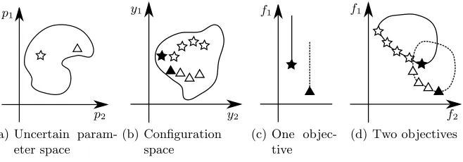
The difference betweenf(x,y⋆_{,p) and f x,y}⋆_,p

spaceP(Fig. 1(a)). The performance of the solution for every scenariop(star or triangle) depends on its configurationy(Fig.1(b)). In Fig.1(c),f1is the only

objective. All possible objective values are bounded by the solid and dashed lines for the star and triangle scenarios, respectively. The black stars and triangles in Figures1(b)and1(c)mark the optimal configuration and objective value for each scenario (y⋆ _{and f(x,y}⋆_{,p), respectively). In Fig.1(d) an additional objective} is considered. Now all possible objective values are bounded by the solid and dashed contours, and the optimal configuration for each scenario consists of a set rather than a single configuration, denoted by the additional white shapes.

p2

p1

(a) Uncertain param-eter space

y2

y1

(b) Configuration space

f1

(c) One objec-tive

f2

f1

(d) Two objectives

Fig. 1.Optimal configurations of a candidate solutionx for two scenarios of the un-certainties, associated with the environmental parameters.

The problem in Eq. (7) is termed here as an Active Robust Multi-objective Optimisation Problem (ARMOP). It introduces a very challenging question:How can adaptable products be evaluated and compared according to their variates of Pareto frontiersF(x,Y⋆,P)?In Section2.1we introduce a first attempt to ad-dress this challenge, and suggest a set-based robustness indicator. In Section4we demonstrate how this indicator can be integrated into an evolutionary algorithm in order to solve an ARMOP.

2.1 Evaluating a Variate of Sets

In order to evaluate a candidate solution for an ARMOP, we suggest using a robustness criterion that quantifies the variate of Pareto frontiers with a single scalar value. Keeping in mind there is no way to avoid the loss of meaningful information when using a scalarising function, we strive to extract as much in-formation as possible regarding the quality of the trade-off surfacesF(x,Y⋆_,P). Following the motivation in evolutionary multiobjective optimisation (EMO), an approximated solution to a MOP is evaluated according to three major qual-ities [18]: proximity of the approximated front to the true Pareto front (PF), diversityof the solutions, andpertinenceto the preferred region of interest.

front and a reference point [19]. The HV measure provides an integrated measure of proximity, diversity and pertinence, although it is sensitive to the choice of a reference point [20]. Despite this drawback, we use it to demonstrate the concept of the robustness indicator suggested in this study.

Hypervolume-Based Robustness Indicator. Without loss of generality, we consider the variatePas a finite set of sampled scenariosp. The HV of solution x for scenario p is denoted as hv(x,p). It is calculated according to the ideal vectorf∗_{and the worst objective vectorf}w_{, which are the vectors with minimum} and maximum objective values, respectively, amongst all known solutions and scenarios. The robustness indicatorIhv is derived as follows:

First, the objectives of f are normalised in a manner that supports DM’s pref-erences (e.g., settingf∗ _{to zero andf}w_{to a vector of weights between 0-1).} Next, the hypervolume hv(x,p) is calculated for each scenario p ∈ P, using the worst objective vector as a reference point. The variate of the hypervolume measure that corresponds to the variatePis denoted asHV(x,P).

Finally, a robustness criterion is used to evaluate the variateHV(x,P):

Ihv[F(x,P)] =I[HV(x,P)]. (8)

Since the aim is to maximise HV(x,P) and its value is bounded between 0-1, in a minimisation problem, the complement can be used:

Ihv[F(x,P)] =I[1−HV(x,P)]. (9)

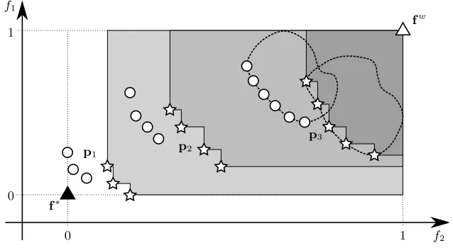
Fig 2 demonstrates the above procedure for a population of two solutions. Three scenarios ofpare considered, where the Pareto frontiers of the two solu-tions are depicted in stars and circles. For scenariop3, dashed contours show the

domains in objective space that include the performances of all evaluated con-figurations. The worst objective vector is calculated according to the objective vectors of all configurations, including non optimal ones. The variateHV x₉,P

is shown as the collection of three HVs forx₉.

3

Case Study – Gearbox Optimisation Problem

0 1 0

1

f2

f1

fw

f∗

p1 p2

p3

Fig. 2.Pareto frontiersF(x,Y⋆

,P) of two solutions (x₉ andx◦) for three scenarios. The ideal vector is marked with a black triangle and the worst objective vector with a white triangle. The hypervolumeshv x₉,p1

,hv x₉,p2

and hv x₉,p3

are shown in the figure.

3.1 Mathematical Model

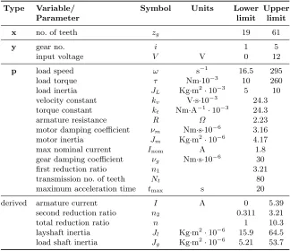
The variables and parameters of the motor and gear system are described in Table1. The values are based on the Maxon A-max 32 DC motor specifications.

At steady state, the power consumption of a geared DC motor is [21]:

P =V ∗I, (10a)

where: I= JL+Jg+n

2

2Jl+n2Jm

˙

ω+ νg+n2νm

ω+τ nkt

, (10b)

V =RI+nkvω. (10c)

When the load is accelerated from rest, it is possible to calculate the speed trajectory, for given trajectories of input voltage and speed reduction, by solving the following differential equation:

˙

ω(t) = n(t)ktV(t)−n(t)

2

kvktω(t)

JL+Jg+n2(t)2Jl+n(t)2Jm

R −

νg+n(t)2νm

ω(t) +τ

JL+Jg+n2(t)2Jl+n(t)2Jm

,

(11)

whereω(0) = 0 is used as a starting condition.

The total energy required for accelerationE can be derived from Eq. (10):

E =

Z T

0

V(t)V(t)−n(t)kvω(t)

R dt, (12)

Table 1.Variables and parameters for the gearbox ARMOP

Type Variable/ Symbol Units Lower Upper

Parameter limit limit

x no. of teeth zg 19 61

y gear no. i 1 5

input voltage V V 0 12

p load speed ω s−1

16.5 295 load torque τ Nm·10−3

10 260 load inertia JL Kg·m

2 ·10−3

5 10 velocity constant kv V·s·10−

3

24.3 torque constant kt Nm·A−

1 ·10−3

24.3 armature resistance R Ω 2.23 motor damping coefficient νm Nm·s·10−

6

3.16 motor inertia Jm Kg·m

2 ·10−6

4.17 max nominal current Inom A 1.8

gear damping coefficient νg Nm·s·10− 6

30 first reduction ratio n1 3.21

transmission no. of teeth Nt 80

maximum acceleration time tmax s 20

derived armature current I A 0 5.39 second reduction ratio n2 0.311 3.21

total reduction ratio n 1 10.3 layshaft inertia Jl Kg·m

2 ·10−6

15.9 64.5 load shaft inertia Jg Kg·m

2 ·10−6

5.21 53.7

3.2 Problem Formulation

According to the ARO methodology, introduced in Section 1.2, the problem variables are sorted in Table1to three types:x,yandp. Most of the parameters in this problem are considered as having deterministic values, but some (ω,τand

JL) possess uncertain values. The random variates of ω, τ andJL are denoted asΩ,T andJL, respectively. The resulting variate ofpis denoted asP.

A gearbox is required to perform well both in steady state and during accel-eration. These two requirements can be considered as different operation modes, with different configuration spaces. The configuration space in steady state in-cludes the choice of the geari and the input voltageV. During acceleration, it consists of trajectories in time of i(t) and V(t). Therefore, the search for the optimal configuration can be separated toy⋆

ss that minimisesP, and toy⋆t that minimisesEandT. Since the latter is a solution to a MOP, it is expected to be a set. The variates ofy⋆

ss andyt⋆ that correspond to the variateP, are denoted asY⋆

Following the above, the AROP is formulated:

min x∈X

h

P(x,Y_ss⋆,P), Ex,Y_t⋆,P, Tx,Y_t⋆,Pi, (13a)

where : Y⋆_ss= argmin y∈Y(x)

P(y,P), (13b)

Y⋆t = argmin y∈Y(x)

[E(y,P), T(y,P)], (13c)

x= [zi], i= 1, . . . ,5, (13d)

y= [i, V], (13e)

P= [Ω,T,JL, kv, kt, R, νm, Inom, νg, n1, Nt, Jm, Jl, JG, tmax], (13f)

s.t.: zg,i+zl,i=Nt, i= 1, . . . ,5, (13g)

Iss≤Inom, (13h)

T ≤tmax. (13i)

The steady state current constraint is evaluated according to Eq. (10b), and the objectives according to Equations (10a), (11) and (12).

Since the ARMOP consists of separable configuration spaces, it can be de-coupled into two subproblems, one that searches forYss⋆ andP(x,Yss⋆ ,P), and another that searches forY⋆

t and

h

Ex,Y⋆ t,P

, Tx,Y⋆ t,P

i

. The former prob-lem is a single-objective AROP, and the latter is an ARMOP. Using robustness indicators, Eq. (13a) can be converted to the following bi-objective problem that simultaneously minimises the steady-state AROP and the transient ARMOP:

min x∈X

"

IhP(x,Y⋆_ss,P)i, Ihv

h

Ex,Y⋆_t,P, Tx,Y_t⋆,Pi

#

. (14)

4

Optimiser Design

The problem was solved by a bi-level EMOA whose structure is described in Algorithm1.

First, the uncertain domain is sampledNptimes. These samples serve as the same representation of uncertainties to evaluate all solutions.

Next, Eq. (13b) is solved for the entire design space, andYss⋆ andP(x,Yss⋆,P) are stored in an archive for every feasible solution. It is possible to find the op-timal steady-state configuration of every solution for all sampled load scenarios because the design space is discrete and the objective and constraints are simple expressions. The search space consists of 962,598 different combinations of gears (choice of 5 gears from 43 possibilities). The constraints and objective functions depend on the number of teeth z, so they only have to be evaluated 43 times for each of the sampled scenarios. A feasible solution is a gearbox that has at least one gear that does not violate the constraints for each of the scenarios (i.e.,

Next, a multi-objective search is conducted amongst the feasible solutions to solve Eq. (14). The solutions to Eq. (13c) for every sampled scenario are obtained by the evolutionary algorithm described in Section 4.1. The solutions to Eq. (13b) are already stored in an archive.

Algorithm 1Pseudo algorithm for solving the ARMOP

sample the uncertain domain

evaluate all possible solutions for steady state (s.s)

initialise nadir and ideal points for transient objectives (limits) generate an initial population

whilestopping criterion not satisfieddo forevery scenariodo

forevery new solutiondo

optimise for time–energy and store PF end for

end for

if limits have changedthen update limits

calculate HV of entire population else

calculate HV of new feasible solutions end if

assign scalar indicator values for s.s and transient

evolve new population (selection, cross-over and mutation) re-mutate solutions that were already evaluated / infeasible for s.s end while

4.1 EMOA for Identifying Optimal Gearing Sequences

For every load scenario, a multi-objective optimisation is conducted for each candidate solution to identify the optimal shift sequence that minimises energy and acceleration time. Early experiments revealed that maximum voltage results in better values for both objectives, regardless of the candidate solution or the load scenario. Therefore, the input voltage was considered as constantVmax, and

the only search variable isi(t), the selected gear at timet. A certain trajectory

i(t) results in a gearing ratio trajectoryn(t) that depends on the gearboxxthat is being evaluated.

The trajectoryi(t) is coded as a vector of time intervalsdt= [dt1, . . . ,dtN] defining the duration of each gear in the sequence from first gear to the Nth, withN being the optimal gear at steady state for the load scenario under con-sideration. The sum of all time intervals is equal to tmax, and this relation is

enforced whenever a new solution is created by setting:

dt← dt

Pluggingn(t) into Eq. (11) results in a trajectoryω(t), which can be used to calculate E,T or whether the gearbox failed to reach the desired speed before

tmax. A multi-objective evolutionary algorithm was used to estimate:

y⋆_t = argmin n(t)

[E(x, n(t),p), T(x, n(t),p)], (16)

where bothxandpare fixed during the entire optimisation run. Solving the differential equation (11) repeatedly to obtainy⋆

t is the most ex-pensive part of the algorithm in terms of computational resources. Therefore, all of the solutions to (16) are stored in an archive to avoid repeated computations.

4.2 Calculating the Set-based Robustness Indicator

The ARMOP’s indicator Ihv uses a dynamic reference point. At every genera-tion, after the approximated Pareto frontiers F(x,Y⋆_{,P) are identified for all} evaluated solutions, the ideal and worst objective vectors are re-evaluated to include the objective vectors of the new solutions. If neither the ideal nor the worst objective vectors have changed,Ihvis calculated only for the recently eval-uated solutions according to the procedure described in Section2.1. Otherwise, the indicator values of the entire current population are recalculated as well, in order to allow for fair comparisons between new and old candidate solutions. No preferences were considered in this case study, hence, the objectives were normalised by settingfw_{to one.}

5

Simulation Results

5.1 Parameter Setting

The ARMOP described in Section3was solved with the proposed evolutionary algorithm. Two robustness criteria were considered:Iw_{considers the worst case} scenario, meaning the upper limits of the uncertain load parameters, as given in Table 1. Im _{considers the mean value over a set of sampled load scenarios.} For both cases the same criterion was used for the steady state and transient indicators of Eq.14, i.e., eitherIw_{and I}w

hv orI

m _andIm

hv.

A standard elitist MOEA [22] with a fixed number of generations was used for both stages of the problem (referred to as outer and inner).

Parameter setting of the outer algorithm: population sizeN = 100, 50 genera-tions, integer coded, One-point crossover with crossover ratepc = 1, polynomial mutation with mutation rate pm= 1/nx= 0.2 and distribution index ηm= 20. Parameter setting of the inner algorithm: population size N = 50, 30 gener-ations, real coded, SBX crossover with crossover rate pc = 1 and distribution index ηc = 15, polynomial mutation with mutation rate pm = 1/ny = 0.2 and distribution indexηm= 20.

5.2 Results

0.3 0.4 0.5 0.6 0.7 0.8 0.9 1 4

6 8 10 12 14

Im

hv[T , E]

I

m[

P

]

[W

]

mean worst−case 0.3 0.35

5.58 5.63 5.68

A

B

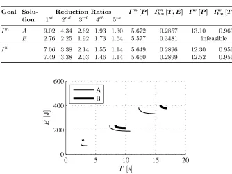
Fig. 3. Approximated Pareto frontiers for the worst-case and mean-value criteria. A close-up of the robust mean Pareto front is shown with the extreme solutions marked asAandB, and the mean performance of the approximated set according toIw_.

The approximated Pareto frontiers for both worst-case and mean-value cri-teria are depicted in Fig.3. For the worst-case criterion, the PS consists of only two, almost identical, solutions. In a close-up view on the approximated PF for mean performance, the extreme solutions are marked as A and B. Mean per-formances of the approximated Pareto set for the worst-case problem are also shown.

Details on the solutions for both robustness criteria are summarised in Ta-ble2. Note the similarity in both design and objective spaces between the two so-lutions of the worst-case problem, and the difference between Soso-lutionsAandB. Also note that the best solutions found for a certain robustness criterion, are dominated for another. SolutionBperforms well in most steady state scenarios, since it has a large variety of high gears (small reduction ratio), but its ability to efficiently accelerate the load is limited from the same reason. SolutionB be-comes infeasible when the worst-case is considered. This was not detected while optimising for the mean value since the worst-case scenario was not sampled. This result highlights the impact of the choice of robustness criterion, and the challenge in optimising for the worst-case (see [3]).

The dynamic performances of SolutionsAandBfor three load scenarios are depicted in Fig 4. SolutionA’s superiority for both dynamic objectives is well captured by theIhv indicator values.

6

Discussion and Future Work

effective-Table 2.Optimisation Results

Goal Solu- Reduction Ratios Im[P] Ihvm[T , E] I w

[P] Ihvw [T , E]

tion 1st ₂nd ₃rd ₄th ₅th

Im _{A 9.02 4.34 2.62 1.93 1.30 5.672 0.2857 13.10 0.9631}

B 2.76 2.25 1.92 1.73 1.64 5.577 0.3481 infeasible

Iw 7.06 3.38 2.14 1.55 1.14 5.649 0.2896 12.30 0.9511 7.49 3.38 2.03 1.46 1.14 5.660 0.2899 12.52 0.9510

0 5 10 15 20

0 200 400 600

T [s]

E

[J

]

A B

Fig. 4.Approximated Pareto frontiersF(x,Y⋆_{,P) of two solutions (AandB) for three}

scenarios (of 25). SolutionAdominates SolutionBin all evaluated scenarios.

ness of design adaptability to improve performance in an uncertain environment. The ARMOP introduces several challenges, some of which were addressed in this study, and others which need to be further explored.

The approach taken in this study to solve an ARMOP is to use a scalarising function to represent the variate of Pareto frontiers of every candidate solution. This approach was found useful for the gearbox case study – solutions with better Pareto frontiers were assigned with a better indicator value. However, whenever a set is represented by a scalar value, some of its information must be lost. As a result, setting a robustness criterion for the utility indicator value does not automatically imply that the individual objectives will also be robust.

evaluations were conducted. It took approximately three days to compute on a 3.40GHz Intelr _CoreTM _{i7-4930K CPU, running Matlab}r _{on 12 cores.}

Future research should explore other representations of the uncertainties that involve more efficient sampling approaches and use of a-priori knowledge; as well as optimisation algorithms for expensive function evaluations. Alternative scalarising functions, and their effects on the optimisation results, should also be explored.

Acknowledgements This research was supported by a Marie Curie Interna-tional Research Staff Exchange Scheme Fellowship within the 7th_European

Com-munity Framework Programme. The first author acknowledges the support of the Anglo-Israel Association.

References

1. Salomon, S., Avigad, G., Fleming, P.J., Purshouse, R.C.: Active Robust Optimiza-tion - Enhancing Robustness to Uncertain Environments. IEEE TransacOptimiza-tions on Cybernetics44(11) (2014) 2221–2231

2. Beyer, H.G., Sendhoff, B.: Robust Optimization - A Comprehensive Survey. Com-puter Methods in Applied Mechanics and Engineering 196(33-34) (July 2007) 3190–3218

3. Branke, J., Rosenbusch, J.: New Approaches to Coevolutionary Worst-Case Op-timization. In Rudolph, G., Jansen, T., Lucas, S., Poloni, C., Beume, N., eds.: Parallel Problem Solving from Nature PPSN X SE - 15. Volume 5199 of Lecture Notes in Computer Science. Springer Berlin Heidelberg (2008) 144–153

4. Avigad, G., Coello, C.A.: Highly Reliable Optimal Solutions to Multi-Objective Problems and Their Evolution by Means of Worst-Case Analysis. Engineering Optimization42(12) (December 2010) 1095–1117

5. Alicino, S., Vasile, M.: An evolutionary approach to the solution of multi-objective min-max problems in evidence-based robust optimization. In: Evolutionary Com-putation (CEC), 2014 IEEE Congress on. (2014) 1179–1186

6. Teich, J.: Pareto-Front Exploration with Uncertain Objectives. In Zitzler, E., Thiele, L., Deb, K., Coello Coello, C., Corne, D., eds.: Evolutionary Multi-Criterion Optimization SE - 22. Volume 1993 of Lecture Notes in Computer Science. Springer Berlin Heidelberg (2001) 314–328

7. Hughes, E.J.: Evolutionary Multi-objective Ranking with Uncertainty and Noise. In Zitzler, E., Thiele, L., Deb, K., Coello Coello, C., Corne, D., eds.: Evolutionary Multi-Criterion Optimization SE - 23. Volume 1993 of Lecture Notes in Computer Science., Springer Berlin Heidelberg (2001) 329–343

8. Deb, K., Gupta, H.: Introducing Robustness in Multi-Objective Optimization. Evolutionary Computation14(4) (November 2006) 463–494

9. Saha, A., Ray, T.: Practical Robust Design Optimization Using Evolutionary Algorithms. Journal of Mechanical Design133(10) (October 2011) 101012 10. Beyer, H.G., Sendhoff, B.: Functions with noise-induced multimodality: a test for

11. Fieldsend, J.E., Everson, R.M.: Multi-objective optimisation in the presence of uncertainty. In: Evolutionary Computation, 2005. The 2005 IEEE Congress on. Volume 1. (2005) 243–250

12. Bui, L.T., Abbass, H.A., Essam, D.: Fitness Inheritance for Noisy Evolutionary Multi-objective Optimization. In: Proceedings of the 7th Annual Conference on Genetic and Evolutionary Computation. GECCO ’05, New York, NY, USA, ACM (2005) 779–785

13. Goh, C.K., Tan, K.C.: An Investigation on Noisy Environments in Evolutionary Multiobjective Optimization. Evolutionary Computation, IEEE Transactions on 11(3) (June 2007) 354–381

14. Knowles, J., Corne, D., Reynolds, A.: Noisy Multiobjective Optimization on a Budget of 250 Evaluations. In Ehrgott, M., Fonseca, C., Gandibleux, X., Hao, J.K., Sevaux, M., eds.: Evolutionary Multi-Criterion Optimization SE - 8. Volume 5467 of Lecture Notes in Computer Science. Springer Berlin Heidelberg (2009) 36–50

15. Fieldsend, J.E., Everson, R.M.: The Rolling Tide Evolutionary Algorithm: A Multi-Objective Optimiser for Noisy Optimisation Problems. Evolutionary Com-putation, IEEE Transactions onPP(99) (2014) 1

16. Paenke, I., Branke, J., Jin, Y.: Efficient Search for Robust Solutions by Means of Evolutionary Algorithms and Fitness Approximation. Evolutionary Computation, IEEE Transactions on10(4) (2006) 405–420

17. Cruz, C., Gonz´alez, J.R., Pelta, D.a.: Optimization in Dynamic Environments: A Survey on Problems, Methods and Measures. Soft Computing 15(7) (December 2011) 1427–1448

18. Fleming, P., Purshouse, R., Lygoe, R.: Many-Objective Optimization: An Engi-neering Design Perspective. In Coello Coello, C., Hern´andez Aguirre, A., Zitzler, E., eds.: Evolutionary Multi-Criterion Optimization SE - 2. Volume 3410 of Lecture Notes in Computer Science. Springer Berlin Heidelberg (2005) 14–32

19. Zitzler, E.: Evolutionary Algorithms for Multiobjective Optimization : Methods and Applications. Phd dissertation, Swiss Federal Institute of Technology Zurich (1999)

20. Knowles, J., Corne, D.: On Metrics for Comparing Nondominated Sets. In: Evolu-tionary Computation, 2002. CEC ’02. Proceedings of the 2002 Congress on, IEEE (2002) 711–716

21. Krishnan, R.: Electric Motor Drives - Modeling, Analysis, And Control. Prentice Hall (2001)