Automated Processing and Analysis of Galactic Neutral Hydrogen Absorption Observations

(1)

Automated Processing and Analysis of Galactic Neutral

Hydrogen Absorption Observations

James Michael Dempsey

A thesis submitted for the degree of

Bachelor of Science with Honours in Astronomy & Astrophysics of The Australian National University

(2)

Declaration

This thesis is an account of research undertaken between February 2016 and October 2017 at The Research School of Astronomy and Astrophysics, ANU College of Physical and Mathematical Science, The Australian National University, Canberra, Australia.

Except where acknowledged in the customary manner, the material presented in this thesis is, to the best of my knowledge, original and has not been submitted in whole or part for a degree in any university.

James M Dempsey October, 2017

(3)

Acknowledgements

Firstly I wish to thank my advisor, Prof Naomi McClure-Griffiths for her guidance and encouragement throughout the project. I have greatly appreciated the way she has always found time in her busy schedule to provide support and advice, and I admire her deep knowledge of the Milky Way.

Thanks also to Dr Jimi Green for use of his data, and assistance with observing information. Finally, thank you to my wife Leanne Dempsey for endless patience, support and editing.

(4)

List of Figures

2.1 Milky Way rotation curve from Benjamin (2017). Positive velocities are shown as red contour lines and negative velocities are shown in blue. The spiral arms are shown in yellow and the dotted straight lines mark Galactic longitude lines. . . 4 2.2 Example emission and absorption spectrum from Murray et al. (2015). This shows the

decomposition of both spectra into Gaussian components. . . 6 2.3 Example beam pattern after five interleaved observations over 12 hours. . . 9

3.1 Distribution of fields observed with fields used shown in red. . . 11 3.2 Plot of the example field 291.270-0.719 with the total intensity (sum of all channels) of

the Hidata on the left and continuum (centred at 1757 MHz) on the right. Both plots show flux density in units of Jy/beam on a linear scale with flux increasing from light to dark. The wedge on the right shows the scale. . . 15 3.3 Chart of fields observed each day and the number of fields which were used. . . 16 3.4 Emission (top) and absorption (bottom) spectra for MAGMOHI G291.277-0.716 against

the background source ‘OH 291.3-0.7’. The continuum region for this Galactic longitude is shown by green dotted lines, the spectrum is in blue and the noise level is in grey. . 17 3.5 Plot of an example spectrum where the parameters produced from training (left)

pro-duced a better fit to the spectrum than the experimentally chosen parameters (right). The grey line is the observed spectrum, the red dashed lines are the individual com-ponents and the blue line is the total of the comcom-ponents. The bottom plot shows the residual values between the Gaussian component totals and the observed spectrum. . . 20 3.6 Plot of our standard example spectrum, MAGMOHI G291.277-0.716. Here, the trained

parameters (left) produced a slightly worse fit for the saturated spectrum than the experimentally chosen parameters (right). . . 20 3.7 Plot of an example spectrum where the parameters produced from training (left)

pro-duced a slightly worse fit for the saturated spectrum than the experimentally chosen parameters (right). . . 20

4.1 Quality metrics for the MAGMO H i spectra (see Section 3.6). The dotted line in the top two plots shows the cut-off value for the test. Both tests are unit-less ratios. . . . 21 4.2 Longitude-velocity diagram of the H i absorption measured by MAGMO. The outline

is the outer range (TB = 1 K) of H i emission measured by GASS (McClure-Griffiths

et al. 2009) . . . 22 4.3 Longitude-velocity diagram of the H i absorption measured by MAGMO for just the

A and B rating spectra. The outline is the outer range (TB = 1 K) of H i emission measured by GASS. . . 22 4.4 Fit for MAGMO absorption spectrum for G331.26-0.19. . . 24 4.5 Left: Optical depth (τ) of each gas component, right: Full width at half maximum for

each component. In both figures, the right bin also contains all components above that value. . . 25

(7)

LIST OF FIGURES vii

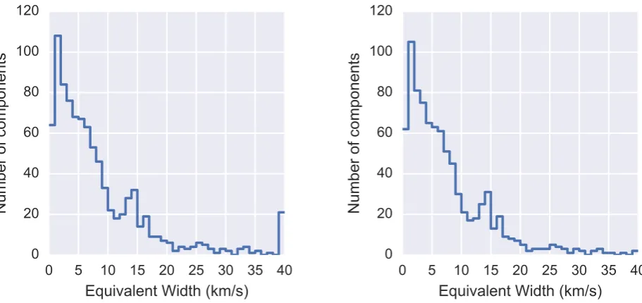
4.6 Left: Histogram of all equivalent width values. Right: Histogram of equivalent width values for just those components with a FWHM <50 km/s. In both figures, the right

most bin contains all components above that value also. . . 26

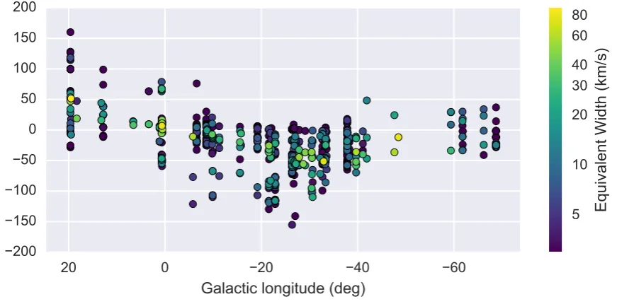
4.7 Equivalent width plotted by Galactic longitude and LSR velocity. The colour denotes equivalent width on a log scale from 0 to 90 km/s with the scale shown in the wedge on the right. . . 27

4.8 Spin temperature plotted by Galactic longitude and LSR velocity. The colour denotes spin temperature on a square root scale from 0 to 300 (or more) K with the scale shown in the wedge on the right. . . 27

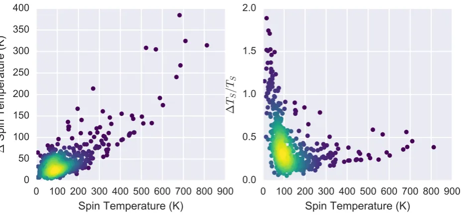
4.9 Left: Spin temperature of each gas component, Right: Column density of each gas component with the total shown in blue and the density of just the saturated spectra shown in red. In both plots, values are only calculated for gas components where we have emission temperature data from SGPS. . . 28

4.10 Left: Plot of the uncertainty in the spin temperatures against the calculated spin tem-peratures. Right: Plot of the same uncertainties expressed as a fraction of the measured spin temperature. . . 28

4.11 Left: Turbulent mach number for each gas component, Right: Fraction of the total gas in the component that is cold. In both cases, values are only calculated for gas components where we have emission temperature data from SGPS. . . 29

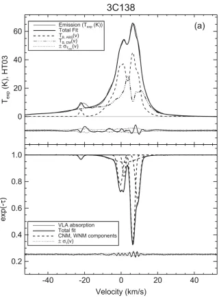
5.1 Comparison of spin temperatures and column densities between this study (blue line) and HT03 (black line). For HT03 the data is limited to the low latitude (|l| <= 10) CNM components . . . 30

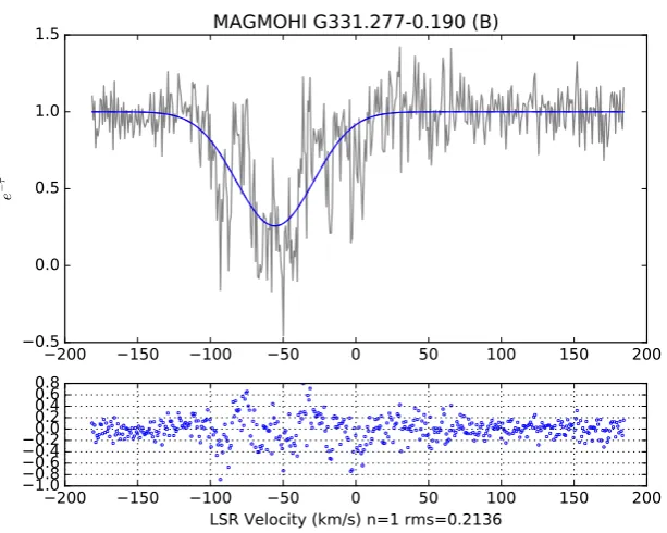
5.2 Fit for MAGMO absorption spectrum for G326.45+0.90. . . 32

5.3 Fit for MAGMO absorption spectrum for G326.65+0.59. . . 33

5.4 Comparison of SGPS and MAGMO absorption spectra for OH 291.3 -0.7. In the left hand panel the MAGMO spectrum, resampled to match the SGPS spectral resolution, is plotted in light blue and the SGPS spectrum in dark blue in front. On the right is the residual taken by subtracting the SGPS spectrum from the MAGMO spectrum. . 34

5.5 Comparison of gas away from (blue line) and near to (black line) the methanol masers in each observed field. Near is defined as within 2 arcmin and ±10 km/s of the maser. Left: Comparison of spin temperatures. Right: Comparison of optical depth (τ). . . . 37

A.1 Comparison of MAGMO and SGPS absorption spectra for GAL 285.25-00.05 . . . 43

A.2 Comparison of MAGMO and SGPS absorption spectra for OH 291.3 -0.7 . . . 43

A.5 Comparison of MAGMO and SGPS absorption spectra for GAL 311.63+00.27 . . . . 44

A.12 Comparison of MAGMO and SGPS absorption spectra for [CH87] 324.954-0.584 . . . 47

A.14 Comparison of MAGMO and SGPS absorption spectra for [DBS2003] 95 . . . 48

(8)

viii LIST OF FIGURES

A.28 Comparison of MAGMO and SGPS absorption spectra for SNR G333.6-00.2 . . . 53

A.40 Comparison of MAGMO and SGPS absorption spectra for HRDS G350.177+0.017 . . 57

A.41 Comparison of MAGMO and SGPS absorption spectra for [KC97c] G350.3+00.1 . . . 57

(9)

Chapter 1

Abstract

In this research project I analysed the composition and structure of the cold neutral hydrogen (H i) gas at the locations of the MAGMO (Mapping the Galactic Magnetic field through OH masers) survey observations. To enable this analysis I developed an automated pipeline and used that to produce Hiabsorption and emission spectra from the MAGMO observations. This pipeline was designed with the aim of being applicable to future large surveys such as GASKAP, the Galactic Australian SKA Pathfinder survey.

The MAGMO observations targeted the sites of 6.7-GHz methanol masers, which are associated with star-forming regions. These very active regions have complex structures with bubbles formed by stellar winds from young, high mass stars. In these regions it is reasonable to expect there will be significant reserves of cold gas. The MAGMO H i dataset provided an excellent opportunity to examine the cold neutral medium (CNM) towards these regions and to compare it with the overall CNM population.

In Chapter 2 I provide a summary of the current knowledge of the Milky Way’s cold H igas and an introduction to other topics which will assist the reader in understanding the analysis. Chapter 3 provides a detailed description of the data, and the pipeline developed for its analysis. This is more detailed than is typical in order to explain the decisions in developing the automated processing. In Chapter 4 I provide the results from the observations. In Chapter 5 I compare the results to results from similar studies, discuss the overall findings and assess the effectiveness of the processing pipeline. Finally in Chapter 6 I summarise the main findings and discuss future potential for both this data set and the processing pipeline.

(10)

Chapter 2

Introduction

2.1 Neutral hydrogen in the Milky Way

Hydrogen, the most abundant element in the universe, fuels stars and is the majority component of the interstellar medium. As a result, understanding its distribution in the galaxy is critical in order to understand the dynamics and history of the galaxy. Observations of neutral hydrogen (HI) have been crucial in mapping the spiral arms of the galaxy (Levine et al. 2006) and, most recently, the mapping of a new outer spiral arm (McClure-Griffiths et al. 2004) in the fourth quadrant of the Milky Way. Such observations have also been used extensively to map the rotation curve of the Galaxy (e.g. Gunn et al. 1979; McClure-Griffiths & Dickey 2016) and to measure kinematic distances of objects within the disc (Jones & Dickey 2012).

Within the Milky Way, H i is located in an exponential disc with a scale height of 3.75 kpc extending out to a Galactic radius R = 35 kpc (Kalberla & Dedes 2008). The disc is warped, with a sine-wave-like vertical shape from R ≥15 kpc. From 40≤R ≤60 kpc a more diffuse and turbulent disc with a scale height of 7.5 kpc is apparent (Kalberla & Dedes 2008). This compares with the thin stellar disc with a scale height of 300−400 pc extending out to∼15 kpc and a thick stellar disc with a scale height of∼1 kpc (Sparke & Gallagher III 2007). Surrounding the centre of the Galaxy there is a 3 kpc radius hole in the H i (Lockman & McClure-Griffiths 2016; Sofue 2017). At a large scale, the H i gas rotates with the galaxy, with gas significantly above and below the disc lagging behind the rotation (Kalberla & Kerp 2009).

Looking closer, there is a wealth of small-scale structure, with abundant shells of H iejected from supernovae and stellar winds, some broken into fragments that appear as sheets or filaments. Even outside of these expanding bubbles the H igas is generally accelerated to typical speeds of 10 km/s (Mach 3) (Heiles & Troland 2003b), indicating that the interstellar medium (ISM) is largely not in equilibrium.

H i gas in the Milky Way is split into two stable phases: the Cold Neutral Medium (CNM) and the Warm Neutral Medium (WNM) (Wolfire et al. 2003). These are two long lasting phases of temperature and pressure equilibrium reflecting the heating and cooling balance in the ISM. The CNM is predominantly dense clouds of Hi gas at temperatures between 40 and 160K. The WNM is generally deemed to be Higas between 4100K to 8800K and is much more diffuse (Murray et al. 2015). Significant gas also occurs in the unstable temperature range between these, however the amount is still contentious, with observations ranging from 48% (Heiles & Troland 2003a) to < 30% (Begum et al. 2010) of WNM and simulations by Kim et al. (2014) predicting 20% to 50%. Table 2.1 shows the commonly understood values for the five stable phases of hydrogen in the Milky Way ISM.

Structurally, the CNM consists of small dense clumps and filaments within the diffuse WNM (Kulkarni & Heiles 1988). These clouds are usually detected in H i absorption and have typical diameters of around 3 parsecs (Kalberla & Kerp 2009). They are dynamic features, forming as cores due to pressure fluctuations in the WNM and then combining into filaments or sheets and dissipating over the course of 105 years (Kalberla & Kerp 2009). They are shaped both by turbulence and by

(11)

§2.2 Radio observations of the CNM 3

magnetic fields. The CNM is found predominantly in the disc of the Galaxy, with a scale height of 150 pc locally, due to the high pressure under which it forms. It makes up 20+7₋₁₀% of Galactic Higas and has column density in the range (4.4±0.5)×1019 cm−2≤ NH≤1×1022 cm−2 (Dickey & Lockman 1990), although Murray et al. (2015) have detected the CNM gas as diffuse as NH≥(3±1)×1016cm−2. Very high sensitivity is needed to detect the lower column density population of CNM.

Phase Name Phase State

of H

Temperature (K)

Density (cm−3)

Filling Factor

mf Mass

Fraction

Hot Ionised Medium HIM H ii 106 10−3 25-65% trace

Warm Ionised Medium WIM H ii 8,000 - 10,000 0.3 25% 15%

Warm Neutral Medium WNM H i 5,000 - 8,000 0.4 35% 35%

Cold Neutral Medium CNM H i 20 - 100 1-50 3% 10%

Molecular Medium MM H2 10 102−6 1% 40%

Table 2.1: Typical Milky Way ISM temperatures and densities for the different phases of hydrogen. The last two columns are the fraction of total ISM hydrogen in each phase by volume and by mass. (Sparke & Gallagher III 2007; Wolfire et al. 2003)

2.2 Radio observations of the CNM

The primary method of observing Hiis radio observation of the 21cm Hispectral line. This hyperfine line is caused by the quantum spin-flip transition of the electron in the neutral hydrogen atom and has a rest frequency of 1,420.40575 MHz (Kulkarni & Heiles 1988). With a transition probability A21 = 2.87×10−15 sec−1 it will be around 12×106 years before an excited H i atom will emit a photon (Kulkarni & Heiles 1988); it does not saturate observations and thus is an excellent means of determining the column density of Hi along a particular line of sight.

There are two broad classes of radio telescopes: single dishes and interferometer arrays. Single dishes generally have a large field of view and a course resolution (e.g. the Parkes 64-metre radio tele-scope has a 14 arcmin FWHM beam at 1420 MHz) while interferometers have a much finer resolution but often have less total collecting area (e.g. the Australia Telescope Compact Array can achieve an 8 arcsec FWHM synthesised beam at 1420 MHz). According to the Rayleigh criterion, the beam width of a telescope is given by the formula:

θ= 1.22λ

d radians, (2.1)

whereλis the wavelength anddis the baseline length (distance between two antenna) or dish radius. This also gives the inverse relationship between the size of structures that the telescopes can detect. Shorter baselines and smaller dishes detect the large-scale structure, while longer baselines give finer resolution, allowing detection of the small structures but at the expense of missing the larger structures. As a result the two telescope types see different scales of structure in the ISM. Single dishes are well suited to seeing the larger structures and observing the 21 cm emission, which is generally produced from extended sources. Interferometers see only the small structures, and due to their finer resolution they are much better at detecting absorption between a source and the telescope. Their lack of zero spacing (extremely short baselines) means they generally do not detect emission from extended sources. More recent surveys of the Milky Way Hihave thus often combined the data from both large dishes and long baseline interferometers.

(12)

4 Introduction

The dip is Doppler-shifted according to the relative velocity of the cloud to the observer, or in our case to the average movement of the stars in the Solar vicinity around the Galactic centre, measured as the Local Standard of Rest (LSR). While this velocity is dominated by the Galactic rotation of the target cloud, the line may be broadened by the motion of the gas within the cloud, or the line-of-sight width of the cloud. A 5 km/s velocity range equates to a distance of 1 kpc for most lines of sight (Burton 1988).

[image:12.595.62.526.320.675.2]

Figure 2.1 shows the rotation curve of the Galaxy. The Galaxy is commonly divided into four quadrants numbered anticlockwise from 1 to 4 starting from longitude 0 (i.e. the first quadrant is the bottom right of Fig. 2.1). In the fourth quadrant of the Galaxy, covering the Galactic longitude range 270 ≤ l < 360, gas inside the solar circle will be moving at negative velocities relative to the LSR. For each line of sight (dotted straight lines in Fig. 2.1) there will be a terminal velocity which is the relative velocity of the innermost Galactic radius that it touches. With a uniform rotation curve it is to be expected that each negative velocity greater than this terminal velocity will be crossed twice, preventing a direct conversion of these velocities into a distance measurement. A similar situation exists for positive velocities in the first quadrant (0< l <90).

Figure 2.1: Milky Way rotation curve from Benjamin (2017). Positive velocities are shown as red contour lines and negative velocities are shown in blue. The spiral arms are shown in yellow and the dotted straight lines mark Galactic longitude lines.

(13)

§2.3 Spin Temperature 5

emission level. For inner galaxy sources this is complicated due to the double crossing of velocity values, so a background source in the inner galaxy in the fourth quadrant could have absorption at velocities more negative than its own LSR velocity if it were located past the terminal velocity point. Where inner galaxy background sources have had their distances determined by other means, such as parallactic distance measurement using Very Long Baseline Interferometry (VLBI), a unique kinematic distance may be determined as some of the far velocities can be excluded.

Near the centre of the Galaxy, the velocities are confused both by velocity crowding and by the non-circular motion of the bar. Within 15◦ of the Galactic centre, the inner galaxy motion is largely perpendicular to the line of sight, so the gas is crowded around a velocity of 0 km/s. Similar velocity crowding occurs near the anti-centre. In the Galactic centre (r <3 kpc), the bulge and bar structure at the centre of the galaxy exhibits solid body rotation resulting in a steep terminal velocity line reaching -250 km/s.

When observing absorption of the H i line we measure the brightness temperature against a background continuum source. To convert this temperature into an optical depthτ we must remove as much of the H i emission as possible and then calculate the ratio of the remaining temperature to the background continuum source’s temperature. This is generally achieved using the following equation,

e−τ(v)= Ton−Tof f Tbg

, (2.2)

whereTonis the brightness temperature when directly observing the source,Tof fis the temperature off

the source, away from the background source andTbg is the brightness temperature of the continuum

background source. The continuum temperature is normally measured at a velocity range where there is no H igas present.

The emission can also be excluded by filtering out the large-scale structure (where most emission comes from), either by Fourier transforming the image and zeroing out the short spacing data, or by observing using long baselines. In these cases there is no need to subtract the Tof f as it is no longer

present in the measuredTon (Dickey et al. 2003).

2.3 Spin Temperature

To calculate the spin, or excitation, temperature TS we need to have emission measurements as well

as the optical depth. The emission is excluded in the longer baselines so it needs to be sourced from shorter baseline or single dish observations. Spin temperature can then be calculated using the following equation.

TS =

Tof f

1−e−τ(v) (2.3)

This gives a density weighted harmonic mean of the temperatures of the clouds along the line of sight at a given velocity. To separate these out we need to account for each component along the line of sight, including the diffuse continuum emission, the cold absorbing gas and warm gas both in front of and behind the cold gas. This leads to the radiative transfer equation of (Dickey et al. 2003, eq. 10)

Tobs(v) =Tw,f+Tw,be−τ(v)+Tcool(1−e−τ(v)) +Tconte−τ(v) , (2.4)

whereTw,f and Tw,b are the apparent temperatures of the foreground and background warm Hi,Tcool

and τ(v) are the temperature and optical depth of the cold H i, and Tcont is the temperature of the

(14)

6 Introduction

There are many methods in the literature for splitting out these components to produce a spin temperature for the cold gas. In general these seek to identify individual components of the absorption spectrum, match those to components in the emission spectrum and then use the emission component to estimate the brightness temperature of the absorption component and then use Eq. (2.3) to estimate the spin temperature.

[image:14.595.61.382.287.722.2]

Many methods start with fitting a sum of Gaussian components to the absorption spectrum, with the intent of reproducing the physical clouds, each of which may be represented by a component (Roy et al. 2013). This hypothesis is supported by the observation that at high Galactic latitudes, non-blended absorption spectra can be quite accurately reproduced as a sum of Gaussians. However in environments such as the Galactic plane where there are overlapping gas clouds, the Gaussian decomposition is not unique and thus multiple solutions are possible (Dickey et al. 2003). Nevertheless this remains the most physically motivated approach to modelling the ISM probed by an absorption spectrum (Roy et al. 2013). An example of such a decomposition is shown in Fig. 2.2.

Figure 2.2: Example emission and absorption spectrum from Murray et al. (2015). This shows the decompo-sition of both spectra into Gaussian components.

(15)

§2.4 H i absorption surveys 7

spectrum is fitted using a sum of Gaussians using a least-squares fitting algorithm. Then the expected emission spectrum is fitted with a combination of the predetermined components for the CNM plus Gaussian components for the WNM. Here the fitting must find both the new Gaussians from the emission but also the spin temperatures from the cold components. Where components overlap, all possible combinations of order are tried to see which one best fits the emission spectrum. The fraction of the warm gas in front of or behind the CNM components are also trialled to find the lowest residuals. Generally the fraction of WNM in front of the CNM does not lead to significantly significant differences in the fit, but is instead used to quantify the errors in the spin temperatures. This approach is also used by Murray et al. (2015) and Stanimirovi´c et al. (2014).

Dickey et al. (2003) describe a two phase linear least-squares fit to the observed emission TB

and absorption e−τ profiles rather than decomposing the spectra into Gaussians. Here they first subtract the background continuum emission from the observed emission spectrum to get a brightness temperatureTB. They then model the emission as a linear function across each individual absorption

component and fit the linear emission and the cool component temperatureTcool−Tcontto the observed

brightness temperature and absorption profile. While different fractions of warm gas in front of the cool gas component are trialled, they generally use the results for a fraction of 0.5 except where it gives an unphysically low spin temperature when they use a fraction of 1, meaning all warm gas is behind the cool cloud. With this approach they avoid the non-uniqueness of Gaussian decomposition for blended lines. A similar approach is used by Strasser et al. (2007) except that they fit a quadratic rather than linear function for the emission.

The final method that Dickey et al. (2003) describe is a two-phase nonlinear least-squares fitting method that aims to provide a continuous solution for the emission either side of the absorption component. In this case they fix the emission at the edges of the absorption component, modelling a linear function between these values, but fitting for the velocity of the component edges for blended absorption components.

Comparisons between iterations of these techniques are made in Heiles & Troland (2003a), Dickey et al. (2003) and Murray et al. (2015). Murray et al. (2015) find that, for their medium and high Galactic latitude sample, the spin temperatures from the Gaussian fitting are closest to the 40≤TS ≤

200K as modelled by Wolfire et al. (2003) for the CNM.

In this study we have opted to implement a limited version of the Gaussian decomposition ap-proach. We decompose the absorption spectra into Gaussian components. However rather than doing the complex full decomposition of the emission spectra we instead simply measure the brightness tem-perature of the cool component as the temtem-perature of the emission spectra at the central velocity of the cool component. This will mean that the calculated spin temperatures will be upper limits rather than actual spin temperatures as some of the emission temperature is likely to have come from warm components rather than just the cool component.

Finally, with a spin temperature and an absorption profile we can calculate the column density NH of the cold component. For the CNM, spin temperature is approximately equal to the kinetic temperature (Dickey & Lockman 1990) so we can substituteTS forTkin the column density equation.

NH= 1.823×1018 cm−2 K−1

Z

Tkτ(ν) dν (2.5)

2.4 H

i

absorption surveys

(16)

8 Introduction

development of large interferometer arrays. Early surveys of Hiabsorption in the Galactic plane used the Arecibo and Greenbank single dish facilities (Dickey et al. 1978) and the Very Large Array (VLA) (Dickey et al. 1983).

In 1999, observations started at the Arecibo observatory for the Millennium Arecibo 21 Centimeter Absorption-Line Survey (Heiles & Troland 2003a). This was a set of long integration time observations of 79 mostly high Galactic latitude bright sources. While the primary objective of the survey was to provide HiZeeman splitting data, the highly sensitive observations provided very high signal to noise H i absorption spectra towards these sources. These were used to analyse the properties of both the CNM and WNM at these specific locations Heiles & Troland (2003b).

In the early 2000s a coordinated effort was made to survey the H i of the Galactic plane. Three surveys were undertaken, the Canadian Galactic Plane Survey (CGPS; Taylor et al. 2003), the VLA Galactic Plane Survey (VGPS; Stil et al. 2006) and the Southern Galactic Plane Survey (SGPS; McClure-Griffiths et al. 2005. These surveys made a huge leap forward in the coverage and detail level of the Galactic H iemission and absorption. They provide coverage of 90% of the galactic disc with a spatial resolution of 2.2 arcmin or better, a velocity resolution of 0.8 km s−1 _{and a 1}_σ _{sensitivity of} 1.6K. There is a gap in coverage in the third quadrant between −170< l < −110◦ which is outside the observed areas of all three surveys, and also at the galactic centre where velocity crowding makes observing far more complex. The improved sensitivity and resolution has revealed new features of the Galaxy such as the previously mentioned new spiral arm and proven an excellent tool in tracing the structure particularly of the outer galaxy (Strasser & Taylor 2004). The surveys have obtained a wealth of absorption spectra, with Strasser et al. (2007) cataloguing spectra towards 793 extragalactic sources and Brown, C et al. (2014) cataloguing absorption features recorded in SGPS towards 252 HII regions.

In the Northern hemisphere, the “21 cm Spectral Line Observations of Neutral Gas with the EVLA” (21-SPONGE Murray et al. 2015) project has achieved new sensitivity levels. It is observing selected very bright sources to obtain optical depth spectra with noise levels of στ = 0.0006 and has

successfully detecting the broad and weak absorption lines from the warm neutral medium.

In the near future, observing for the Galactic ASKAP survey (GASKAP; Dickey et al. 2013) will commence. GASKAP will cover the Southern sky, covering quadrants 3 and 4. It will provide a factor of 5 increase in the number of absorption spectra recorded withστ ≤0.05 over previous surveys such

as SGPS and will achieve optical depth noise ofστ ≤0.02 for sources of S = 50 mJy. It aims to record

absorption at a 10 arcsec spatial resolution, 0.206 km/s velocity resolution and a 1σ sensitivity of 2K at the highest resolutions.

2.5 Interferometry Observations

A short summary of some important radio interferometry concepts is useful for understanding some of the compromises and decisions made in this work.

A radio interferometer consists of multiple antennae observing a region of sky simultaneously. Each pair of antennae forms a baseline, so

nbaselines=nantennae(nantennae−1) (2.6)

A delay time, based on the length of the baseline, is used to adjust the amplitudes from one antenna in each baseline so that the radiation received from the target sky region interferes constructively. This is termed the cross-correlation of the the two amplitudes.

(17)

§2.6 Processing Pipelines 9

GHz.

[image:17.595.345.540.194.349.2]

With discrete antennae separated by large distances, the instantaneous sampling of the sky is sparse. Due to the cross-correlation between antennae the sampling is actually of the Fourier transform of the sky brightness, theu-vplane. As we are sampling in the Fourier domain, the largest structures are seen only in the shortest baselines. As most emission comes from the larger structures our power is also affected by the baseline length choice.

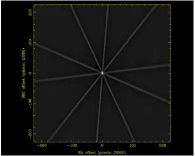
Figure 2.3: Example beam pattern after five interleaved observations over 12 hours.

In an East-West array such as the ATCA, we rely on Earth rotation synthesis to improve the sampling. Over a period of hours the angle of the array changes with respect to the sky region being observed, thus the array will make a more complete sample of the u-v plane. This also affects the beam shape, as with an instantaneous sampling from an East-West array the beam is just a line in theu-vplane. As the array rotates with respect to the sky, a more circular region of the u-v plane is sampled and the beam becomes less elongated. So ideally we would observe for 12 hours to get optimal u-v coverage. However given the need to balance telescope time with coverage, we often interleave observations of multiple fields over time e.g. field a, phase cal, field b, phase cal, field c, phase cal, field a, phase cal etc. This will sample theu-v plane at different angles with the aim being to evenly sample 180 degrees. Figure 2.3

shows the result of such an interleaved observing pattern for a field.

The noise levels of an observation of a point source with an interferometer are governed by the radiometer equation (Johnston & Gray 2006, eq. 6):

σs∝

Tsys

ApN(N −1)Bt , (2.7)

where σS is the rms of the noise level for a point source,Tsys is the system noise temperature of the

telescope,A is the area of one antenna,N is the number of antenna in the array,B is the bandwidth of each sample in Hertz and t is the integration time in seconds. This means that wider bandwidth and longer integration times result in lower noise. The collecting area of the dish also affects the noise levels of the observation, with a smaller antenna receiving less emission, thus increasing the relative noise level.

The most commonly used data format for radio interferometry data is the visibility format. This format stores the response for each baseline in the u-v plane. This needs to be combined with cali-bration data and then imaged using Fourier transformation. Asu-v plane sampling is sparse we also need to clean the data to reduce effects from bright sources such as sidelobes.

2.6 Processing Pipelines

When reducing small volumes of data, the general approach used has been for each astronomer to have their own set of scripts generally doing a step at a time and leaving some steps as interactive. Of course, processing toolkits such as Miriad, AIPS and CASA have been around for a long time and do much of the heavy lifting for data reduction. However as the volume of data being produced by surveys increases, these techniques are not sufficient to keep up.

(18)

10 Introduction

automated data reduction pipelines, with LoFAR (van Haarlem et al. 2013) setting up imaging and pulsar pipelines for automated data reduction, ASKAP creating ASKAPsoft (Cornwell et al. 2011) to accomplish imaging and spectra extraction from the raw visibilities. Individual surveys are also examining automated pipelines, such as the current work on the DALiuGE framework (Wu et al. 2017) for the CHILES (Fern´andez et al. 2016) project.

One area that has emerged as a non-trivial and important problem is source finding (Hopkins et al. 2015). A variety of source finding toolkits have emerged in response to this such as Aegean (Hancock et al. 2012), and Selavy (Whiting & Humphreys 2012).

2.7 The MAGMO Survey

The MAGMO survey was an Australia Telescope Compact Array observing program run from 2010 to 2012 which had the aim of studying “Magnetic fields of the Milky Way through OH masers” (Green et al. 2012b). It was primarily concerned with measuring Zeeman splitting of hydroxyl (OH) ground state spectral lines. Many of the OH masers observed by the MAGMO survey were associated with 6.7 GHz methanol masers. These emissions are linked to high mass star formation (HMSF) regions (Minier et al. 2003). As a secondary objective, neutral hydrogen observations were taken towards most of the same sources (Green et al. 2010). As a result these H i observations will be largely of HMSF regions.

While the OH maser data has been partially analysed in (Green et al. 2012b) and processing of the rest of the OH data is in progress, the H idata has not been processed and analysed previously.

2.8 The MAGMO-H

i

Project

In the current work we have taken the MAGMO Hiabsorption data, created an automated processing pipeline, and used it to reduce and analyse the data. The analysis was twofold. First, we evaluated the effectiveness of the pipeline, including comparing both new and previously observed sight-lines with previous observations. Secondly, we calculated major characteristics of the observed H i, compared them against previous studies and examined what this widespread absorption dataset tells us about the observed Hi.

This project extends the SGPS analysis of the Southern Galactic plane in three ways.

Firstly, as it will utilise automated Gaussian decomposition, it will allow the automatic decom-position results to be compared to the carefully decomposed absorption spectra of the SGPS. This comparison will inform the analysis strategies of the upcoming GASKAP project.

Secondly, the absorption-only MAGMO data will allow verification of the subtraction of emission spectra in the SGPS to produce absorption spectra.

Thirdly, with a Galactic longitude range more extended than SGPS, this project will provide absorption data for regions not covered in the SGPS nor in other Galactic plane surveys.

(19)

Chapter 3

Data Analysis

3.1 The MAGMO Observations

Between January 2010 and June 2012, 644 observations were made of 440 targets with the ATCA, including repeats for observations affected by equipment issues, Radio Frequency Interference (RFI) and weather. The observations are all targeted at sites of 6.7 GHz methanol masers observed during the methanol multibeam survey (Green et al. 2012a). The targets of the observations are shown in Fig. 3.1 with a background image of the Milky Way H i intensity from the HI4PI survey (HI4PI Collaboration et al. 2016).

180°

240°

300°

0°

60°

120°

Galactic Longitude

-30°

+0°

+30°

Galactic Latitude

Figure 3.1: Distribution of fields observed with fields used shown in red.

In addition to the OH observations, the ATCA’s zoom mode was used to obtain simultaneous high spectral resolution observations (2048 channels each 0.5 KHz wide) of Hiwith a ∼400 km/s velocity coverage, along with a continuum band (2049 channels each 1 Mhz wide centred on 1757 MHz) (Green et al. 2010). The observations were all at low galactic latitudes (|b| ≤2.9) and covered the longitude range 188◦ to 19◦. As the 6 km baseline configuration of the ATCA was used, the HI observations have a spatial resolution of 7.5”. Each source was observed for a total of 30 minutes, in 5 scans of 6 minutes each across a 12-hour observing period.

While this is not highly sensitive, it is sufficient for detecting HI absorption. and is slightly more sensitive than the SGPS, which took 20 minute observations of each source. The observations also have higher angular resolution than the SGPS. Due to the higher angular resolution, the MAGMO noise levels will be slightly higher than SGPS, despite SGPS only taking 20 minute observations of each source. The MAGMO scans were interspersed with calibration observations and observations of other sources.

The response from each pair of antennas, or baselines, was recorded in a raw visibility format as described in Section 2.5.

(20)

12 Data Analysis

Listing 3.1: ADQL query to return all MAGMO observation files with H_idata

SELECT o b s i d , c o n f i g u r a t i o n , number scans , f r e q u e n c y , a c c e s s e s t s i z e , a c c e s s u r l

FROM i v o a . o b s c o r e

WHERE o b s c o l l e c t i o n = ’ C2291 ’ and f r e q u e n c y in ( 1 4 2 0 , 1 4 2 0 . 5 , 1 4 2 1 ) GROUP BY o b s i d , c o n f i g u r a t i o n , number scans , f r e q u e n c y ,

a c c e s s e s t s i z e , a c c e s s u r l

3.2 The MAGMO Data

The uncalibrated visibility data are held in the RPFITS1 format in the Australia Telescope On-line Archive (ATOA). These files can be listed using the ATOA Table Access Protocol service at

http://atoavo.atnf.csiro.au/tap with the query shown in Listing 3.1

Each file contains data for Hi, continuum and OH observations for targets and calibration sources. In total for the 43 half days of observing, 1.6TB of data were generated.

The processing of this data, as described in the rest of this chapter, produces the following data products:

• Continuum Image– a FITS format image of each field from the 1757 MHz centre band, with a 1 arcsec resolution, generally covering a 19x19 arcmin area

• Hi Image Cube– A FITS format image cube of selected fields with spatial and velocity axes, with a 5 arcsec spatial resolution and a 0.8 km/s spectral resolution, generally covering a 32x32 arcmin area and a -250 to 250 km/s Hivelocity range

• Hi Absorption Spectra– VOTable format tables of the optical depth vs velocity for selected background continuum sources

• Catalogues– VOTable format tables of the details of each field, continuum source, continuum island, H ispectrum, H iGaussian component and H igas component

• Preview Images– PNG format preview images of each continuum image, Hiimage cube and H ispectrum

All data are available on request and will be published in conjunction with a paper which is under preparation.

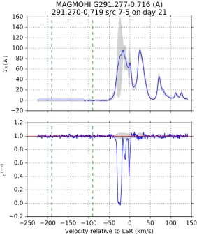
Throughout this thesis we will be using the field ’291.270-0.719’ which was observed on 10 Sep 2011 (day 21), as an example. From that field, the spectrum ’MAGMOHI G291.277-0.716’ against the background source ’OH 291.3-0.7’ will be used as an example spectrum. As detailed in Section 3.5, the spectra are named after the Galactic longitude and latitude of their location.

3.3 Data Reduction Strategy

Processing large volumes of data brings a scaling problem which often breaks traditional processing models. Typically an astronomer would have a set of scripts which they modify and run for each data file, or which list the specific data files and commands to be be run. The maintenance of these becomes onerous at large volumes, particularly where a change in approach or parameters may result in the need to change many copies of the same commands. When exploring large data sets it can be

(21)

§3.3 Data Reduction Strategy 13

essential to be able to tweak parameters and then rerun the processing to see the effect on the results, as well as to be able to run the pipeline on new data files such as the latests observational results. This has led to the introduction of configurable pipelines for processing large survey datasets as detailed in Section 2.6.

We have implemented such a pipeline with the aim of automating all steps wherever possible and to be simple to rerun in order to incorporate new data and tune the process. This also al-lowed the processing to be easily repeated both to ensure reproducibility and to allow different set-tings to be compared. The MAGMO-HI pipeline, as used for producing this thesis, is available at doi:10.5281/zenodo.1036733.

As noted earlier, due to the emphasis on testing the automation of processing, the processing is described in greater detail than typical in this section. This allows for the assessment of the effectiveness of various parts of the automation. It also facilitates the independent reproduction of the results presented in this thesis.

The pipeline was split into phases to allow the tasks to be rerun individually. The main phases were:

• find data – Identify the RPFITS data files to be downloaded from ATOA

• load data – Extract the required data from the RPFITS files for a specified day

• process day – Flag, calibrate, produce 2 GHz continuum images and H i image cubes for a specified day

• analyse data – Identify sources and extract spectra for a specified day

• analyse spectra – Aggregate all spectra, assess quality, produce reports, diagrams and catalogues

• decompose – Decompose each spectrum into a sum of Gaussian components

• examine gas – Calculate physical characteristics of the gas and compare it with results from other studies

While process day and analyse data, in particular, operate on data volumes that require use on larger processing servers, the analyse spectra and later tasks can operate on the lower volume output data products using a normal laptop.

Notable tasks automated for this study included:

• Automatic flagging of the 0 km/s region in the 1420 MHz bandpass calibrator data

• Filtering the fields to be used for spectra extraction based on exclusion of both duplicate obser-vations and poor quality obserobser-vations

• Source finding using theAegeanpackage

• Selection of sources at which spectra will be extracted

• Extraction of emission data around the sources from the SGPS data

• Fitting Gaussian components to the absorption spectra

(22)

14 Data Analysis

While many of these were non-trivial to prepare generalised solutions for, in combination they mean that the pipeline can run without manual intervention and process large volumes of data efficiently.

The pipeline was also designed with traceability of results in mind. The observing day, field and source identifications as well as the spatial location were recorded with each spectra. As the source identification may change as the input continuum images were refined, a position-based identifier was also assigned to each spectrum to allow traceability.

To facilitate traceability the VOTable format (Ochsenbein et al. 2013) was used for recording any tabular data such as catalogues and spectra. This is a flexible container for tabular data that allows for full metadata to be held with the data. It has wide support including inAstropy (Astropy Collaboration et al. 2013) and TOPCAT (Taylor 2005), both of which were extensively used in the production of this work. The use of Virtual Observatory compatible data exchange formats also allows the easier publication and reuse of the data.

Some areas remained which required human intervention. The largest of these was the flagging of known bad data. The list of time, frequencies, sources and fields that should be flagged and ignored was manually curated based on the observing log and manual examination of the diagnostic plots. This meant that there was limited flagging of the target source data and the phase calibrator data.

A potential future improvement for the phase calibrator data would be to automatically identify time periods where the fluxes vary from the expected flat amplitude, or show excessive polarisation. These time periods could then be dynamically flagged. This would automatically filter out short term RFI in the phase calibrator observations. As the target sources may have some variability, this approach would not be usable on those data without the risk of losing valid results.

The processing was mostly single-threaded. Using appropriate infrastructure, the processing prob-lem would be amenable to parallel processing. A simple approach would be to run the process data and analyse data steps on a number of days in parallel. This would require minor modification to the control scripts and also testing to ensure that this doesn’t slow down the overall result due to I/O contention, or exceeding the memory or CPU capacity of the processing server.

3.4 Miriad Processing

The Miriad (Sault et al. 1995) tool suite was used to extract, calibrate and image the data. A standard Miriad recipe was followed to produce continuum FITS images and 3D Hiimage cubes from the visibility data. The main steps involved were:

1. Convert the RPFITS format data to Miriad’s visibility format and extract the data of interest.

2. Flag the data that was known to be invalid. A combination of set rules (e.g. amplitude>500 Jy and the 200 channels at the edges), and a curated list of known bad data was used. In addition the local HI absorption was excluded from the bandpass calibration data by flagging the 110 channels around a LSR velocity of 0 km/s. Finally values more than 3 sigma from the mean in the phase calibrator data were also flagged.

3. Produce bandpass, flux calibration and phase calibration solutions and apply them to the con-tinuum and Hi data.

4. Fourier invert the continuum visibility data from the u-v plane into the image plane.

(23)

§3.4 Miriad Processing 15

6. Restore the continuum image by convolving the clean image with a Gaussian representation of the beam and adding it to the residual image.

7. Identify which fields would have sufficient signal to noise to be worthwhile producing H icubes.

8. Average the Hidata to 0.8 km/s spectral resolution to improve the signal-to-noise ratio.

9. Repeat steps 4 through 6 for the H i data to Fourier invert, clean and restore the H i image cubes.

10. Output the continuum images and Hi image cubes into FITS format.

The configuration used in many of the steps had to be iteratively refined to produce optimal images and data cubes. The quality of the output data was assessed using metrics such as the signal to noise ratio of the final images/cubes, noise levels in the non absorbed velocity ranges of bright background sources and the errors and warnings reported during the processing. Examples of modifications made were the flagging of phase calibrator data where RFI was apparent, and the selection of an appropriate clean function and parameters.

We split the steps for bulk processing into two Python scripts,load-data.pyandprocess_day.py. The first script implemented step 1 as this has little configuration or requirement to be rerun. The second script covered the steps 2 – 10, which need to be rerun either partially or completely each time the configuration is modified. In addition, numerous diagnostic images and web pages are produced by the process_day.py script to allow manual verification of the performance of each step and the end products.

Figure 3.2: Plot of the example field 291.270-0.719 with the total intensity (sum of all channels) of the Hi

data on the left and continuum (centred at 1757 MHz) on the right. Both plots show flux density in units of Jy/beam on a linear scale with flux increasing from light to dark. The wedge on the right shows the scale.

(24)

16 Data Analysis

Figure 3.3: Chart of fields observed each day and the number of fields which were used.

3.5 Source Finding and Spectra Extraction

Absorption spectra require the use of a bright background source against which to extract the spectra. To find these background sources we can either use a pre-existing catalogue, or search images of the region for sources. As we had commensal continuum observations available for the H i observations we decided to use these to find suitable sources as they would best reflect the available data. However as described in Section 2.6 source finding is a non-trivial process and as a result we have chosen to use a dedicated source finding package.

Spectra from the MAGMO dataset are produced by identifying sufficiently strong background sources, extracting the flux values at each velocity step at the position of the source, and then dividing the flux by the continuum to produce a spectrum in optical depth units. This process is implemented in theanalyse_day.py program and run on the data one day at a time.

We have used the Aegean package Hancock et al. (2012) to identify the sources from the 1757 MHz continuum images. This is a two-step process, with the BANE function first being used to assess the noise levels in each region of the image. The outputs from this are then input intoAegean, along with the continuum FITS image to assess sources. We then filter the identified sources to just those with a signal-to-noise ratio (S/N) ≥10 and a flux density ≥20 mJy. Each accepted source is given an identifier of the form MAGMOHI Glll.lll+b.bbbfor ease of later reference, wherel is the Galactic longitude and bis the Galactic latitude, both in decimal degrees.

At the position of each of the sources in this filtered list we then use astropy (Astropy Collabo-ration et al. 2013) and numpy to extract a subcube from the HI image cube around the source. The World Coordinate System (WCS) implementation within Astropy is used to convert the sky position of the source into a pixel position within the image cube. Then a subset of the image cube is taken along the velocity axis of a 5x5 grid around the central source pixel position. The pixels that are not within the ellipse of the source component are zeroed out leaving just the pixels within the source. This subcube is the calibrated flux density across the source at each velocity step.

(25)

§3.5 Source Finding and Spectra Extraction 17

as the continuum flux for that pixel.

The continuum flux of each pixel is used to calculate the integrated spectrum for the source according to the following equation.

1−e−τ(v)=X

i "

c2_i

P jc2j

!

si(v) #

, (3.1)

where ci is the continuum flux for theith pixel and si(v) is the flux of the pixel at the velocity step.

This is based on (Dickey et al. 1992, eq. 2) although it is important to note that the data used here is not continuum subtracted. Finally the flux values at each velocity position are divided by the average continuum level to produce a spectrum of optical depthe−τ as shown in Eq. (2.2).

Emission data are sourced from the SGPS dataset. A set of 6 points, located 60◦ apart in a circle of radius 1.08 arcmin (half of the SGPS beam width) is selected. If the point is within any detected island, or has significantly negative emission (TB ≤ −12 K), it is moved away from the source location

by another half a beam width and this is repeated until it satisfies both criteria. If a point reaches more than ten beam widths from the source then the point is discarded. An emission spectra, in brightness temperature units of K, is extracted from the SGPS data at each specified point. The mean and standard deviation for each velocity step across all of the used points is calculated, with the mean being used as the emission spectra and the standard deviation as the emission noise.

20

0

20

40

60

80

100

120

140

160 T

B

(

K

)

MAGMOHI G291.277-0.716 (A)

291.270-0.719 src 7-5 on day 21

250 200 150 100

50

0

50 100 150

Velocity relative to LSR (km/s)

0.2

0.0

0.2

0.4

0.6

0.8

1.0

1.2 e

(

−

τ

[image:25.595.67.350.385.723.2]

)

(26)

18 Data Analysis

The pipeline then writes out a VOTable format file for each source with the spectrum in both flux and optical depth units along with general information on the source such as position and identity. It also produces a plot of the emission and optical depth spectra, an example of which is shown in Figure 3.4.

Longitude Range (deg) Velocity Range (km/s)

0 to 60 -180 to -120

61 to 180 100 to 160

181 to 300 -190 to -90

301 to 310 -200 to -120

311 to 360 120 to 180

Table 3.1: Velocity ranges used to identify the continuum flux level at different galactic longitudes

3.6 Spectra Analysis

The spectra analysis stage, which we implemented in theanalyse_spectra.pyprogram, was the first of the pipeline stages where the full set of spectra were processed as a whole data set. This stage filtered out duplicate fields and sources, compiled catalogues, assessed the quality of the spectra and produced plots for further analysis.

Each spectrum file was read in and was then automatically assessed for quality using the following quality tests from Brown, C et al. (2014).

• Range – Check that the range (e−τ)<1.5, reflecting that the optical depth should be between 0 and 1.

• Maximum signal to maximum noise – Check the ratio of maximum signal to maximum noise (1−min(e−τ))

(max(e−τ₎₋₁₎≥3.

• Baseline noise – check the noise level in the continuum region of the absorption spectrum, 3σcontinuum <1.

This results in a rating scale of A – D, with rating A spectra passing all tests and rating D spectra failing all tests.

We then filtered out duplicate spectra. These occur when overlapping fields contain the same sources. Any two sources with a separation of less than four arc seconds were considered duplicates and the poorer quality source was flagged and excluded from further processing. Poorer quality was indicated by a worse quality rating, or for the same rating, a higher baseline noise level.

The pipeline then wrote out the compiled list into a VOTable format file magmo-spectra.vot

which included additional file metadata to allow the spectra files and their plots to be linked to each catalogue entry. This enabled us to use tools such as TOPCAT (Taylor 2005) to visually explore the spectra.

Similarly the field metadata files written out in the first steps by process_day.pywere read in by the pipeline, and a combined catalogue of the fields was written out tomagmo-fields.vot.

3.7 Decomposition of the Spectra

(27)

§3.7 Decomposition of the Spectra 19

each spectrum has been fitted individually by manually determining the number and approximate position of the Gaussians and using a least-squares fitting algorithm to optimise the Gaussian param-eters to fit the spectrum. In this study we trialled the use of the Autonomous Gaussian Decomposition (AGD) algorithm as implemented ingausspy (Lindner et al. 2015). It is important to note that the decomposition is not unique and that for most spectra there will be multiple possible solutions. AGD automates the standard fitting approach by making the initial estimate of the Gaussians and then applying a least-squares-fit algorithm to produce the final Gaussian components.

AGD was initially trialled on very high signal to noise 21-SPONGE absorption spectra at high Galactic latitudes by Lindner et al. (2015) with good results. Since then it has been used in a comparison with simulated data by Murray et al. (2017) and achieved a recovery rate of 0.53 for low latitude absorption components. The recovery rate is a measure of the algorithm’s effectiveness. It is the number of components identified by the AGD compared to the number identified by a manual decomposition by an expert. The lower recovery rate for the low latitude spectra is largely due to the complex and overlapping nature of the components in this environment. Thus with our lower signal to noise spectra of low latitude environments we can expect that there will be limitations in the recovery of components.

As is standard for machine learning techniques, AGD needs to be trained on representative data with known solutions before it is applied to new data.

We generated a sample training dataset of 50 synthetic spectra. Each spectrum was 512 channels wide, and was composed of 4 Gaussians with random parameters in the ranges of 4 – 35 channels wide, 0.25 to 1.25 amplitude, and positioned between 35% and 75% along the spectrum plus a normal distribution random noise with a 1σ noise level of 0.05. This simulates a set of spectra in 1−e−τ space, each with four potentially overlapping components plus noise.

Gausspyincludes two approaches to finding the initial components. These are the a) total variation approach, where the first to fourth derivatives of the signal are used to find local minima of the curvature and b) convolution approach, where the data is convolved with a Gaussian filter prior to calculating the derivative. We used the convolution approach, as implemented with the conv mode, as this provides the best performance for spectra with significant noise. In this mode the alpha value determines the size of the Gaussian kernel used to filter the data. The training routine was run multiple times with varying seedα1 and α2 values to determine to where it would converge. The best matches to the training data were obtained when the alpha values converged onα1= 4.36,α2 = 9.37 so these values were used for the decomposition.

In the decomposition process, we read in all rating A and B spectra which were not duplicates, convert the spectra to 1−e−τ _{values and then saved them in an internal format for}_gausspy_{to process.}

We then passed in the selected alpha values, and a required signal to noise threshold (5) to gausspy

which processes all spectra in one run. This generally took under 5 minutes to process all 385 spectra. To check the results of the decomposition we compared the results of the trained decomposition values with an alternative set chosen by experimentation. The alternative alpha values wereα1= 3.5, α2= 4.36 . The trained values performed better for the noisier rating B spectra, with a mean residual difference (residualexperimental −residualtrained) of 0.02±0.06. However for the rating A spectra,

(28)

20 Data Analysis

200 150 100 50 0 50 100 150 200 0.2 0.0 0.2 0.4 0.6 0.8 1.0 1.2 e − τ

MAGMOHI G000.679-0.028 (A)

200 150 100 50 0 50 100 150 200 LSR Velocity (km/s) n=7 rms=0.0706

0.3 0.2 0.1 0.0 0.1 0.2

0.3 150 100 50 0 50 100 150 200

0.2 0.0 0.2 0.4 0.6 0.8 1.0 1.2 e − τ

MAGMOHI G000.679-0.028 (A)

150 100 50 0 50 100 150 200 LSR Velocity (km/s) n=4 rms=0.1581

0.5 0.4 0.3 0.2 0.1 0.0 0.1 0.2 0.3 0.4

Figure 3.5: Plot of an example spectrum where the parameters produced from training (left) produced a better fit to the spectrum than the experimentally chosen parameters (right). The grey line is the observed spectrum, the red dashed lines are the individual components and the blue line is the total of the components. The bottom plot shows the residual values between the Gaussian component totals and the observed spectrum.

60 40 20 0 20

0.2 0.0 0.2 0.4 0.6 0.8 1.0 1.2 e − τ

MAGMOHI G291.277-0.716 (A)

60 40 20 0 20

LSR Velocity (km/s) n=3 rms=0.0583 0.25 0.20 0.15 0.10 0.05 0.00 0.05 0.10 0.15

0.20 60 50 40 30 20 10 0 10 20 30

0.2 0.0 0.2 0.4 0.6 0.8 1.0 1.2 e − τ

MAGMOHI G291.277-0.716 (A)

60 50 40 30 20 10 0 10 20 30 LSR Velocity (km/s) n=6 rms=0.0324

0.10 0.05 0.00 0.05

Figure 3.6: Plot of our standard example spectrum, MAGMOHI G291.277-0.716. Here, the trained parameters (left) produced a slightly worse fit for the saturated spectrum than the experimentally chosen parameters (right).

120 100 80 60 40 20 0 20 40 60 0.2 0.0 0.2 0.4 0.6 0.8 1.0 1.2 e − τ

MAGMOHI G327.304-0.550 (A)

120 100 80 60 40 20 0 20 40 60 LSR Velocity (km/s) n=6 rms=0.1073

0.4 0.3 0.2 0.1 0.0 0.1 0.2 0.3 0.4

0.5 100 80 60 40 20 0 20 40

0.2 0.0 0.2 0.4 0.6 0.8 1.0 1.2 e − τ

MAGMOHI G327.304-0.550 (A)

100 80 60 40 20 0 20 40

LSR Velocity (km/s) n=8 rms=0.0496 0.10 0.05 0.00 0.05 0.10 0.15

(29)

Chapter 4

Results

4.1 Spectra

In total, we extracted 819 spectra towards unique sources in this study. Of those, 559 were of sufficient quality to be plotted (rating A – C) and 238 were suitable for decomposed (rating A – B). The quality assessment and distribution by rating of the spectra is shown in Fig. 4.1

A B C D

10-2

10-1

100

101

102

σ

cont

in

uu

m

Baseline Noise

A B C D

10-1

100

101

102Max Signal:Max Noise

A B C D

Quality Rating

0 50 100 150 200 250 300 350

Number

Figure 4.1: Quality metrics for the MAGMO H _i spectra (see Section 3.6). The dotted line in the top two plots shows the cut-off value for the test. Both tests are unit-less ratios.

Absorption was detected in all of these sight lines. The distribution of the absorption is shown in Fig. 4.2. Notably, all of the rating A – C spec-tra contained velocity ranges with deep absorption where e(−τ) < 0.25, reflecting the ubiquity of cold Higas at low latitudes. This can be seen in Fig. 4.2 as all longitudes have some bright points.

In Fig. 4.3 we can see that the absorption points in the higher quality spectra are confined to the ve-locity regions where neutral hydrogen emission was observed in the GASS data (McClure-Griffiths et al. 2009). In the fourth quadrant (−90 < l < 0◦) the absorption traces the inner Galaxy terminal velocity line well atv <0 km/s.

Comparing Figs. 4.2 and 4.3 we can see that the exclusion of the rating C spectra gives a much lower noise level and still has coverage of much of the sur-vey region. For this reason, further analysis is con-fined to just the rating A and B spectra.

While most of the gas observed is in the inner

Galaxy we do observe some outer Galaxy H igas (outer is where the Galactic radius is greater than that of the solar circle). In the −70< l < −45◦ region we see absorption both in the inner and the outer Galaxy. Some absorption in the outer Galaxy can be expected, as while the fields are targeted towards Galactic sources, any other sufficiently bright continuum sources in the field will also be used as background sources for spectra. If these sources are extragalactic (e.g. quasars) then their light may be absorbed by cold Hi clouds in the outer Galaxy.

The limited observations of the first Galactic quadrant cover only the inner Galaxy, with almost all absorption in the first quadrant of Fig. 4.3 being in positive velocities.

(30)

22 Results

-120

-100

-80

-60

-40

-20

0

20 Galactic longitude (deg)

300

200

100

0 -100

-200

-300

LSR Velocity (km/s)

Longitude-Velocity

0.15

0.30

0.45

0.60

0.75

0.90

[image:30.595.62.489.119.362.2]

e

(−τ)

Figure 4.2: Longitude-velocity diagram of the H_iabsorption measured by MAGMO. The outline is the outer

range (TB = 1 K) of Hiemission measured by GASS (McClure-Griffiths et al. 2009)

-120

-100

-80

-60

-40

-20

0

20 Galactic longitude (deg)

300

200

100

0 -100

-200

-300

LSR Velocity (km/s)

Longitude-Velocity

0.15

0.30

0.45

0.60

0.75

0.90 e

(−τ)

Figure 4.3: Longitude-velocity diagram of the H i absorption measured by MAGMO for just the A and B

[image:30.595.66.489.467.714.2]

(31)

§4.2 Analysis of the gas 23

4.2 Analysis of the gas

The 238 unique rating A and B spectra were decomposed into Gaussian components using GaussPy. In total, 922 components were identified, hence an average of four components per spectrum. In four cases, GaussPy failed to identify any components for the spectra. All of these were rating B spectra with significant noise. An example of the gas characteristics are shown in Table 4.1.

4.2.1 Gaussian Components

The distribution of optical depth and full width at half maximum (FWHM) of the identified compo-nents are shown in Fig. 4.5. The prevalence of saturated velocity ranges in the spectra is reflected in the components, with slightly more than 15% havingτ >3, which is generally regarded as saturated (e−τ <0.05). The FWHM distribution shows that most components are narrow, with the peak at 5 – 7.5 km/s, reflecting the population of small cold clouds with low internal velocities. This is quite similar to the typical width of 7 km/s given by Dickey & Lockman (1990) for the CNM. There is a significant tail of very wide components which physically imply clouds that either have very high-temperature or are very extended along the line of sight. Both of these are unlikely for cold gas and at the sensitivity of this survey, so a more likely explanation is that multiple narrower components have been fitted as a single component, an example of which can be seen in Fig. 4.4. This is possible when noise obscures the form of components, or where there is strong saturation which causes the line to expand.

Noise in optical depthτ scales according toστ×eτ (Dickey & Lockman 1990). As a result saturated

regions are much more affected by noise than optically-thin regions. Given the continuum noise in the spectra and the deep absorption within the Galactic plane, the exp(−τ) values can be pushed into the negatives where the log function diverges, so the fitting to Gaussians was done inexp(−τ) space. When the spectra was saturated or negative, the exp(−τ) value was limited to 1×10−16 to calculate theτ value, setting a limit of 36.8 on theτ values.

The equivalent width for each Gaussian component was calculated as (1−exp(−τ)) × FWHM. The overall distribution of values is shown in the left-hand panel of Fig. 4.6. Much like the FWHM, while 91% of the values were less than 20 km/s, there was a long tail of high values reaching up to a maximum of 280 km/s. These higher values came from the high FWHM values previously discussed, and the highest occurred where there were multiple components fitted with a single broad and deep component. Excluding records with a FHWM≥50 km/s, as shown on the right of Fig. 4.6, restricts the highest equivalent width to 45.46 km/s, again highlighting that these are not broad shallow components as expected for absorption in the warm neutral medium.

The distribution of the values by longitude and velocity is shown in Fig. 4.7. The high equivalent width values are most apparent in the regions where the gas is crowded and there are very close or overlapping components, precisely the areas that are hardest to decompose into individual components.

Name Velocity

(km/s)

Optical Depth

FWHM

(km/s) TS (K) NH cm

−2 _M

t

MAGMOHI G291.277-0.716A -25.26 -0.14 9.93 81.9±73.3 5.82×1022 10.3

MAGMOHI G291.277-0.716B -1.41 0.47 3.66 133.0±50.0 7.19×1020 2.2

MAGMOHI G291.277-0.716C -11.68 0.65 4.36 228.1±64.0 8.38×1020 _1.9

Automated Processing and Analysis of Galactic Neutral Hydrogen Absorption Observations