The Legendre Wavelet Method for Solving Singular Integro-differential Equations

(1)

The Legendre Wavelet Method for Solving Singular Integro-differential

Equations

Naser Aghazadeh, Y. Gholizade Atani and P. Noras

Department of Applied Mathematics, Azarbaijan Shahid Madani University, Tabriz 53751 71379, Iran. E-mail:[email protected]

Abstract In this paper, we present Legendre wavelet method to obtain numerical solution of a singular integro-differential equation. The singularity is assumed to be of the Cauchy type. The numerical results obtained by the present method compare favorably with those obtained by various Galerkin methods earlier in the literature.

Keywords. Legendre wavelet, Singular integro-differential equation, Operational matrix.

2010 Mathematics Subject Classification. 65T60, 45E05.

1. Introduction

The singular integro-differential equation

2dφ

dx +λ Z 1

−1

φ(t)

t−xdt=f(x), −1< x <1, λ >0 (1.1)

with specified end conditions,φ(±1) = 0, and a special forcing functionf(x) =−x

2,

was solved earlier by frankel [3], Chakrabarti and Hamsapriye [2], and recently by

Mandal and Bera [7].

Applications in many important fields, like fracture mechanics [5], elastic contact

problems [1], the theory of porous filtering [4] and combined infrared radiation and

molecular conduction [3], contain integral and singular integro-differential equation

with singular kernel. The solution of some of these problems may be obtained

ana-lytically by the method introduced in [9].

The forcing functionf(x) =−x

2, is importance case, because it arises in the study

of problems concerning conduction and radiation. Also singular integro-differential equations arise in connection with solving some special type of mixed boundary value problems involving the two dimensional Laplace’s equation in the quarter plane. Here we applied Legendre wavelets for solving such singular integro-differential equation.

The numerical results show that the method has good accuaracy. We suppose thatφ

isL2_[₋₁_,_{1] function and also Holder continuous.}

(2)

2. Legendre wavelet

In recent years, wavelets have found their place in many applications such as signal processing, image processing, and solution of many equations. The main characteristic of wavelets is its ability to convert the given differential and integral equations to a system of linear or nonlinear differential equations, which are then solved by existing numerical methods.

Wavelets constitute a family of functions constructed from dilation and translation of a single function called the mother wavelet. When the dilation parameter ’a’ and the translation parameter ’b’ vary continuously, we have the following family of continuous wavelets as:

ψa,b(t) =|a| −1

2 ψ(t−b

a ), a, b∈R, a6= 0.

If we restrict parameters a and b to discrete values as:

a=a−k

0 , b=nb0a−0k, a0>1, b0>0,

wheren, kare positive integers then we have the following family of discrete wavelets:

ψk,n(t) =|a| −1

2 ψ(ak

0t−nb0),

whereψk,n(t) form a basis forL2(R).

Legendre waveletsψnm(t) =ψ(k,n, m, tˆ ) have four arguments:

ˆ

n= 2n−1, n= 1,2,3, . . . ,2k−1

, k∈Z+,

wheremis the order of Legendre polynomials andtis the normalized time. They are

defined on the interval [0,1) as

ψnm(t) = ( q

m+1 22

k

2pm(2kt−ˆn) nˆ₂−k1 ≤t < ˆ

n+1 2k ,

0 otherwise, (2.1)

where m = 0,1,2, . . . , M −1, n = 1,2,3, . . . ,2k−1_{. The coefficient} q_m₊1

2 is for

orthonormality, the dilation parameter is a= 2−k _{and translation parameter is} _b ₌

ˆ

n2−k_.

Here pm(t) are well-known Legendre polynomials of orderm with the aid of the

following recurrence formulas:

p0(t) = 1,

p1(t) =t,

pm+1(t) =t

₂ m+ 1

m+ 1

pm(t)−

m m+ 1

(3)

3. Function approximation

A functionf(t) defined over [0,1) may be expanded using Legendre wavelet as

f(t) = ∞

X

n=1 ∞

X

m=0

cnmψnm(t), (3.1)

wherecnm=hf(t), ψnm(t)i, and h., .idenotes the inner product. If the infinite series

(3.1) is truncated, then it can be written as

f(t)∼= 2k₋₁

X

n=1

M−1

X

m=0

cnmψnm(t) =CTΨ(t), (3.2)

where C and Ψ(t) are 2k−1_M _×_{1 matrices given by}

C= [c10, c11, . . . , c1_M−1, c20, . . . , c2_M

−1, . . . , c2k₋₁₀, . . . , c₂k₋₁

M−1]

T_, _(3.3)

Ψ = [ψ10, ψ11, . . . , ψ1_M−1, ψ20, . . . , ψ2_M₋1, . . . , ψ2k₋₁0, . . . , ψ2k₋₁_M−1]T. (3.4)

Also a two variables functionh(t, s)∈L2_([0_,₁₎_×_[0_,_{1)) can be written as:}

h(t, s)≃ΨT(t)HΨ(s),

whereH is 2k−1_M_×₂k−1_M _{matrix with}

Hij = (ψi(t),(h(t, s), ψj(s))).

3.1. The operational matrices of derivative. The differentiation of vectors Ψ in

(3.4) can be expressed as

Ψ′

(x) =DΨ(x), (3.5)

whereDis operational matrix of derivative for Legendre wavelets. If we assume that

k= 1, vectors Ψ and differential of vectors Ψ can be written as follows

Ψ(t) = [ψ10(t), ψ11(t), . . . , ψ1M−1(t)], (3.6)

Ψ′

(t) = [ψ′ 10(t), ψ

′

11(t), . . . , ψ ′

1M−1(t)]. (3.7)

The matrixD can be obtained by the following process:

d(i, j) = Z 1

0

ψ′

1i(t)ψ1j(t)dt, j= 1, . . . , i−1 (3.8)

d(i, j) = 0, j_≥i. (3.9)

4. Applying the method

The Legendre wavelet method terminology is used in [11] in 2001 by Razzaghi et al.

Also, many authors, e.g. [10,17–19] have handled Legendre wavelets for the solution of

varieties of differential and integral equations. Venkatesh et al. in [6,12–16] applied

(4)

in [6] Legendre wavelet method used for numerical solutions of partial differential equation.

In the present article, we are concerned with the application of Legendre wavelets

to find the approximate solution of Eq. (1.1). The Legendre wavelet method (LWM)

consists of reducing the given integral equations to a system of simultaneous nonlinear equations. The properties of Legendre wavelets are utilized to evaluate the unknown coefficients and find an approximate solution to the equation.

The unknown functionφ(x) of (1.1) with φ(±1) = 0, can be represented in the

form

φ(x) =p1−x2_g₍_x₎_, ₋₁_≤_x_≤₁_,

where g(x) is a well behaved function ofx in the interval−1 ≤x ≤1. To find an

approximate solution of (1.1), g(x) is approximated using Legendre wavelets in the

interval [−1,1] as

g(x) = 2k₋₁

M−1

X

j=0

cjψj(x), (4.1)

with consideringk= 1 we can write

g(x) =CTΨ(x), (4.2)

where

CT = [c0, c1, . . . , cM−1], (4.3)

ΨT _{= [}

ψ0, ψ1, . . . , ψM−1], (4.4)

and with the above notification we have following expression for thef(x) as

f(x) =FT_Ψ(_x₎_, _(4.5)

where

FT = [f0, f1, . . . , fM−1]. (4.6)

Substituting (4.1) in (1.1), we get

2 d

dx

(1−x2)12g(x)

+

Z 1

−1

(1−t2₎1 2g(t)

t−x dt=f(x). (4.7)

Define vectorV as follows

V = Z 1

−1

p

1−t2ψ0(t)

t−xdt, . . . , Z 1

−1

p

1−t2ψM−1(t)

t−x dt T

. (4.8)

Now Eq. (4.7) can be written in matrix form

2p1−x2_CT

DΨ(x)−CT√ x

1−x2Ψ(x) +λC

T

V =FTΨ(x), (4.9)

whereD is the operational matrix of derivative. We collocate Eq.(4.9) inM

colloca-tion points, thus we haveM equations andM unknown coefficientscj:

2q1−x2

iC T

Dψ(xi)−CT xi 1−x2

i

ψ(xi) +λCTV(xi) + xi

(5)

fori= 0, . . . , M−1. We solve thisM nonlinear equations by the Newton iterative

method. Then the unknown coefficients cj can be found, so the problem is solved

numerically.

5. Numerical results

In order to illustrate the performance of our method in solving integro-differential equations, we consider the following examples. The solution of the examples are

obtained for different values ofN.

Example1. Here we solve Eq. (4.9) forλ= 1 andf(x) =−x

2. Using these coefficients

the value off(x) at x = (0.2)k, k = 0,1,· · ·,5, are presented in Table 1. For a

comparison between the present method and that of the method used in [3], values

of φ(x) at these points obtained by Frankel [3] are also given. It is obvious that

the result compares favorably with the results of Frankel and also those obtained by

Chakrabarti and Hamsapriye [2] and Mandal and Bera [7]. It was further observed

that by increasingM the accuracy of the result increases.

Table 1. _{Numerical results for example 1}

0 0.2 0.4 0.6 0.8 1

n=6 0.06982 0.0669 0.06007 0.04718 0.02876 0

n=8 0.06976 0.06745 0.06002 0.04718 0.02795 0

n=10 0.06966 0.06703 0.06053 0.04717 0.02850 0

frankel 0.06950 0.06712 0.05984 0.04718 0.02891 0

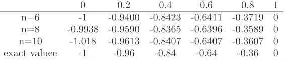
Example 2. Consider the following integro-differnential equation [8]:

φ′(s) + 1

π5

Z 1

−1

φ(t)

t−sdt=

2(1 +π5₎_s

π5 +

(s2₋₁₎

π5 ln

1−s

1 +s

, (5.1)

with the exact solution φ(s) = s2₋_{1. Table} ₂ _{gives the numerical results for this}

example.

0 0.2 0.4 0.6 0.8 1

n=6 -1 -0.9400 -0.8423 -0.6411 -0.3719 0

n=8 -0.9938 -0.9590 -0.8365 -0.6396 -0.3589 0

n=10 -1.018 -0.9613 -0.8407 -0.6407 -0.3607 0

exact valuee -1 -0.96 -0.84 -0.64 -0.36 0

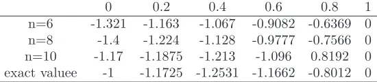
Example 3. Consider the following integro-differential equation:

dφ ds +

Z 1

−1

φ(t)

t−sdt= (s

2_{+ 2}

s−1)es+e1−s

(6)

0 0.2 0.4 0.6 0.8 1

n=6 -1.321 -1.163 -1.067 -0.9082 -0.6369 0

n=8 -1.4 -1.224 -1.128 -0.9777 -0.7566 0

n=10 -1.17 -1.1875 -1.213 -1.096 0.8192 0

exact valuee -1 -1.1725 -1.2531 -1.1662 -0.8012 0

with the exact solutionφ(s) = (s2−1)es. Table3 gives the numerical results of the

method.

These examples show the efficiency and accuracy of the method. Table2and Table

3 show the exact value off(x) ats= (0.2)k, k= 0,1,· · ·,5, and the values of φat these points obtained by presented method.

References

[1] V. Alexandrov and E. Kovalenko,Problems with mixed boundry conditions in continuum me-chanics, Nauka, Moscow, 1986.

[2] A. Chakrabarti and Hamsapriye,Numerical solution of a singular integro-differential equation, ZAMM Z. Angew. Math. Mech.,79(1999), 233–241.

[3] J. I. Frankel,A Galerkin solution to a regularized Cauchy singular integro-differential equation, Quart. Appl. Math.,53(1995), 245–258.

[4] M. Hori and S. Nemat-Nasser,Asymptotic solution of a class of strongly singular integral equa-tions, SIAM J. Appl. Math.,50(1990), 716–725. DOI 10.1137/0150042.

[5] A. C. Kaya and F. Erdogan,On the solution of integral equations with strongly singular kernels, Quart. Appl. Math.,45(1987), 105–122.

[6] N. Liu and E.-B. Lin,Legendre wavelet method for numerical solutions of partial differential equations, Numer. Methods Partial Differential Equations,26(2010), 81–94. DOI 10.1002/num. 20417.

[7] B. N. Mandal and G. H. Bera,Approximate solution of a class of singular integral equations of second kind, J. Comput. Appl. Math.,206(2007), 189–195. DOI 10.1016/j.cam.2006.06.011. [8] A. Mennouni, The iterated projection method for integro-differential equations with Cauchy

kernel, J. Appl. Math. Inform.,31(2013), 661–667. DOI 10.14317/jami.2013.661. [9] N. I. Muskhelishvili,Singular integral equations. 1953, Noordhoff, Groningen.

[10] M. Razzaghi and S. Yousefi, Legendre wavelets method for the solution of nonlinear prob-lems in the calculus of variations, Math. Comput. Modelling, 34 (2001), 45–54. DOI 10.1016/S0895-7177(01)00048-6.

[11] M. Razzaghi and S. Yousefi,The Legendre wavelets operational matrix of integration, Internat. J. Systems Sci.,32(2001), 495–502. DOI 10.1080/002077201300080910.

[12] S. Venkatesh, S. Ayyaswamy, and S. Raja Balachandar,Legendre approximation solution for a class of higher-order volterra integro-differential equations, Ain Shams Engineering Journal,3

(2012), 417–422.

[13] S. Venkatesh, S. Ayyaswamy, and S. Raja Balachandar,Legendre wavelets based approximation method for solving advection problems, Ain Shams Engineering Journal,4(2013), 925–932. [14] S. G. Venkatesh, S. K. Ayyaswamy, and S. Raja Balachandar,Convergence analysis of Legendre

wavelets method for solving Fredholm integral equations, Appl. Math. Sci. (Ruse),6 (2012), 2289–2296.

(7)

[16] S. G. Venkatesh, S. K. Ayyaswamy, S. Raja Balachandar, and K. Kannan,Legendre wavelets based approximation method for Cauchy problems, Appl. Math. Sci. (Ruse),6(2012), 6281–6286. [17] S. Yousefi and M. Razzaghi, Legendre wavelets method for the nonlinear Volterra-Fredholm integral equations, Math. Comput. Simulation,70(2005), 1–8. DOI 10.1016/j.matcom.2005.02. 035.

[18] S. A. Yousefi,Legendre wavelets method for solving differential equations of Lane-Emden type, Appl. Math. Comput.,181(2006), 1417–1422. DOI 10.1016/j.amc.2006.02.031.