https://doi.org/10.5194/angeo-36-1207-2018 © Author(s) 2018. This work is distributed under the Creative Commons Attribution 4.0 License.
Multiscale variation model and activity level estimation algorithm
of the Earth’s magnetic field based on wavelet packets
Oksana V. Mandrikova1,2, Igor S. Solovyev1,2, Sergey Y. Khomutov3, Vladimir V. Geppener4, Dmitry M. Klionskiy4, and Mikhail I. Bogachev5
1Laboratory of System Analysis (LSA), Institute of Cosmophysical Research and Radio Wave Propagation, Far Eastern Branch of the Russian Academy of Sciences, Paratunka, Kamchatka region, Russian Federation 2Kamchatka State Technical University, Petropavlovsk-Kamchatsky, Russian Federation
3Geophysical Observatory, Institute of Cosmophysical Research and Radio Wave Propagation, Far Eastern Branch of the Russian Academy of Sciences, Paratunka, Kamchatka region, Russian Federation
4Computer Science Department, Saint Petersburg Electrotechnical University “LETI”, Saint Petersburg, Russian Federation
5Department of Radio Engineering, Saint Petersburg Electrotechnical University “LETI”, Saint Petersburg, Russian Federation
Correspondence:Dmitry M. Klionskiy ([email protected])
Received: 17 December 2017 – Revised: 2 August 2018 – Accepted: 11 August 2018 – Published: 19 September 2018
Abstract.We suggest a wavelet-based multiscale mathemat-ical model of geomagnetic field variations. The model is par-ticularly capable of reflecting the characteristic variation and local perturbations in the geomagnetic field during the peri-ods of increased geomagnetic activity. Based on the model, we have designed numerical algorithms to identify the char-acteristic variation component as well as other components that represent different geomagnetic field activity. The sub-stantial advantage of the designed algorithms is their fully automatic performance without any manual control. The al-gorithms are also suited for estimating and monitoring the activity level of the geomagnetic field at different magnetic observatories without any specific adjustment to their par-ticular locations. The suggested approach has high temporal resolution reaching 1 min. This allows us to study the dynam-ics and spatiotemporal distribution of geomagnetic pertur-bations using data from ground-based observatories. More-over, the suggested approach is particularly capable of dis-covering weak perturbations in the geomagnetic field, likely linked to the nonstationary impact of the solar wind plasma on the magnetosphere. The algorithms have been validated using the experimental data collected at the IKIR FEB RAS observatory network.
Keywords. Magnetospheric physics (storms and sub-storms)
1 Introduction
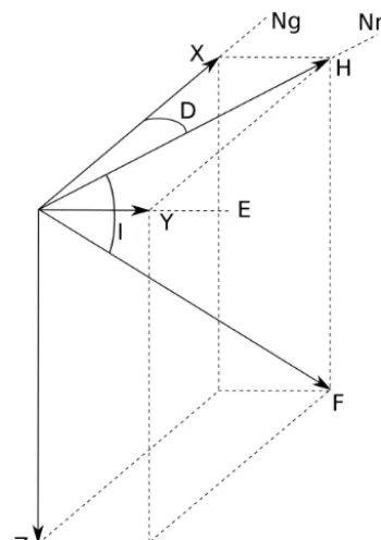
The Earth has its own magnetic field, which is also widely known as the geomagnetic field (also called “the Earth’s ge-omagnetic field” or “the Earth’s magnetic field”) (Bartels et al., 1939). The Earth’s magnetic field varies continuously with both time and ambient space and can be represented as a superposition of the main field, the local field, and the variable field (Zaitsev et al., 2002). The above elements of the Earth’s magnetic field are typically described using the rectangular coordinate system, where the axes are directed towards north, east, and downwards (Fig. 1).
The Earth’s magnetic field vector can be represented ei-ther by componentsX,Y andZ in the Cartesian reference system with axes to geographical north, east, and vertically downwards, respectively, or by componentsH (horizontal),
D(declination) andZin the cylindrical system. Another al-ternative is using componentsF (total intensity), D andI
(inclinations) in the spherical system.H points to magnetic north,Dis the angle between the geographical and magnetic meridians and is positive to the east, whileI is the angle be-tween the horizontal component and the intensity vector.
mag-Figure 1.Geomagnetic field components.
netic storms. The observed temporal variations in the Earth’s magnetic field vector components are referred to here as the geomagnetic signals.
This paper is particularly focused on the development of analysis techniques for geomagnetic signal fluctuations char-acterizing the complex spatiotemporal structure and dynam-ics of the variable geomagnetic field. The variable part of the field is induced by the corpuscular flows of the magnetized plasma emanating from the Sun along with solar wind. De-tailed characterization of the fluctuation phenomena in obser-vational geomagnetic signals at multiple scales from global effects to local perturbations is essential for the understand-ing of the intensity, type, and development of a magnetic storm.
The complex structure of geomagnetic signals and an in-sufficient number of adequate mathematical models make these data difficult to analyze using manual techniques. Con-ventional approaches mainly employ basic time-series analy-sis models and methods that include various smoothing oper-ations (smoothing and trend extraction, Chen, 2007; Joselyn, 1979; Rangarajan, 1989; Sucksdorff et al., 1991). Periodic changes and patterns in the data are typically analyzed using traditional Fourier techniques (Berryman, 1978; Golovkov et al., 1989). However, observational geomagnetic signals are often nonstationary and exhibit a heterogeneous multiscale structure (e.g., Consolini et al., 2013; Klausner et al., 2013). Therefore conventional analysis techniques (smoothing and trend extraction, Fourier techniques), while being able to pro-vide a rather general picture, result in the smoothing of the local perturbations that often contain important information
about geomagnetic field activity and are explicitly associated with the development of magnetic storms.
To overcome the above limitations, we suggest here a spe-cialized nonlinear approach to the analysis of the geomag-netic signals that is based on the wavelet transform (Mallat, 1999; Holschneider, 1995). In this paper, we studied vari-ations in the geomagnetic field and estimated their charac-teristics using the approach based on wavelet packets and first suggested in the papers from Mandrikova et al. (2012, 2013b). Nowadays wavelets and wavelet packets are among the most frequently applied mathematical tools in signal pro-cessing (e.g., Hafez et al., 2010; Jach et al., 2006). Regard-ing applications in geophysics and, in particular, the Earth’s magnetic field studies, we would like to emphasize some of the most significant advantages of wavelet-based approaches (Jach et al., 2006; Kumar and Foufoula-Georgiou, 1997; Mandrikova et al., 2011; Nayar et al., 2006; Rotanova et al., 2006; Xu et al., 2008):
– Wavelets and wavelet packets are capable of tracking the multicomponent structure of the observational ge-omagnetic data, considering that gege-omagnetic signals exhibit multiscale features. The local multiscale com-ponents are largely hindered by trends, thus altogether constituting a complex signal structure.
– Unlike wavelets, wavelet packets are a more flexi-ble signal processing tool. Wavelets work only with a low-frequency component at each decomposition level and leave a high-frequency one unchanged. In con-trast, wavelet packets act to decompose both the high-frequency and the low-high-frequency components at each decomposition level, providing better resolution and finer splitting of the time–frequency domain.
– Wavelets and wavelet packets provide fast computa-tional techniques for finding wavelet coefficients. These techniques are very important for processing long and/or high-resolution data sets.
[image:2.612.78.253.63.311.2]properties and characteristics of the waves of ultra-low fre-quency (ULF) of the magnetosphere (Balasis et al., 2012, 2013, 2015), and studying characteristics of solar daily vari-ations based on data from ground-based magnetic stvari-ations (Klausner et al., 2013), as well as several other issues. Ad-ditional applications of wavelets include the estimation of different geomagnetic activity indices such as the K index (Mandrikova et al., 2012, 2013b), Dst index and the wavelet-based index of storm activity “WISA” (Jach et al., 2006; Xu et al., 2008).
Recently, a multiscale analysis of geomagnetic data has been applied to reveal the anisotropic and nonintermittent character of geofields, helping to distinguish between their strong and wide-range variability (Lovejoy et al., 2001). Fur-thermore, nonlinear effects have been described in the frame-work of multifractal models with particular applications to multifractal and magnetization fields (Pecknold et al., 2001). Additional applications of multiscale analysis to the geomag-netic field include descriptions of its long-term horizontal in-tensity variation, which are capable of tracking its intermit-tency and representing a more complex nature of geomag-netic response to solar wind changes than previously thought (Consolini et al., 2013).
The model proposed here is based on multiscale wavelet analysis and allows us to study characteristic variations in the geomagnetic field and nonstationary short-term changes characterizing fast-flowing processes in the magnetosphere. We also discuss how this model can facilitate an in-depth analysis of geomagnetic field variations. Previously we have shown that the wavelet-based multiscale model allows us to automate the procedure of determining the “quietest” days for calculating the Sq variation and K index by using the Bartels technique (Bartels et al., 1939) and automatic extrac-tion and estimaextrac-tion of perturbaextrac-tions in the geomagnetic field (Mandrikova et al., 2013a, 2014). In this paper, in order to perform a more detailed analysis of the geomagnetic data and study nonstationary short-term variations in the geomagnetic field, we suggest an enhanced version of this model. We dis-cuss the potential area of application of the suggested model and some practical techniques based on this model. Using a prominent example of the analysis of geomagnetic data from a network of ground-based stations, we demonstrate the po-tential of the suggested approach for studying variations in the field and extracting subtle features during periods of in-creased geomagnetic activity.
The paper is organized as follows. In the “Data used in the study” section, we provide data used in the research and in-formation about the observatories registering these data. The section also contains information on the analyzed magnetic storms. In the “Material and methods” section, we provide a brief theoretical outline of our wavelet-based approach, in-cluding the suggested multiscale model and associated algo-rithms to assess characteristic variations and local perturba-tions in the geomagnetic field during periods of increased geomagnetic activity. In the “Experimental results and
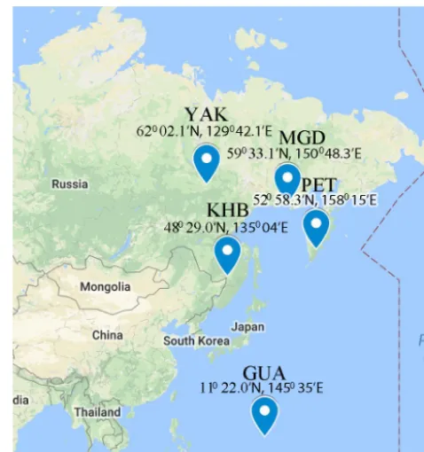
dis-Figure 2.Geographical position of observatories that provided data used in this study.
cussion” section, we validate our model and algorithms using the observational data obtained at magnetic observatories of Institute of Cosmophysical Research and Radio Wave Prop-agation (IKIR) and Y. G. Shafer Institute of Cosmophysical Research and Aeronomy (IKFIA) of the Russian Academy of Sciences and Guam observatory (United States Geologi-cal Survey). In the “Conclusions” section, we have provided the main results of our research.
2 Data used in the study
Experiments were carried out using the geomagnetic data (horizontal component of the magnetic field) obtained at the IKIR observatories Paratunka (PET), Magadan (MGD) and Khabarovsk (KHB) (in the eastern region of Russia). Additional data sets for the analysis were kindly offered by the Yakutsk (YAK) observatory of the IKFIA (Siberian region of Russia). Magnetic data from the Guam obser-vatory were obtained from INTERMAGNET (GUA, http: //www.intermagnet.org; last access: 30 August 2018) and used for the analysis of the equatorial magnetospheric pro-cesses. More detailed information on the geographical loca-tion of the observatories is represented inF Fig.1 and Table 1.
[image:3.612.309.548.65.320.2]Table 1.Observatories whose data were used.
Observatory IAGA Geographical Geographical Geomagnetic Geomagnetic Local time
code latitude (N) longitude (E) latitude (N)∗ longitude (E)∗ (LT)
Yakutsk YAK 62◦02.10 129◦42.10 52◦26.40 163◦130 UTC+09
Magadan MGD 59◦33.10 150◦48.30 51◦32.40 146◦2.40 UTC+11
Paratunka PET 52◦58.30 158◦15.00 45◦51.60 137◦57.60 UTC+12
Khabarovsk KHB 48◦29.00 135◦04.00 39◦150 15◦48.60 UTC+10
Guam, USA GUA 11◦22.00 145◦35.00 3◦730 142◦340 UTC+10
∗Geomagnetic coordinates were calculated using the IGRF model (Thebault et al., 1964;
http://wdc.kugi.kyoto-u.ac.jp/igrf/gggm/index.html; last access: 30 August 2018).
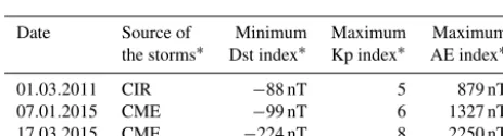
Table 2.The characteristics of the magnetic storms analyzed in the paper.
Date Source of Minimum Maximum Maximum the storms∗ Dst index∗ Kp index∗ AE index∗
01.03.2011 CIR −88 nT 5 879 nT 07.01.2015 CME −99 nT 6 1327 nT 17.03.2015 CME −224 nT 8 2250 nT
∗Tables have been formed using the following data: The catalogue of ICMES by Ian
Richardson and Hilary Cane,
http://www.srl.caltech.edu/ACE/ASC/DATA/level3/icmetable2.htm (last access: 30 August 2018); Space Weather Prediction Center,
ftp://ftp.ngdc.noaa.gov/STP/swpc_products/daily_reports (last access: 30 August 2018); International Service of Geomagnetic Indices (ISGI) http://isgi.unistra.fr (last access: 30 August 2018).
long-term artificial and manmade effects and calculated by the standard Gaussian filtering of raw values.
The results of our analysis were compared with data from the interplanetary magnetic field and the parameters of solar wind (http://www.srl.caltech.edu/ACE/ASC/index.html; last access: 30 August 2018). In order to analyze geomagnetic activity in the auroral zone, we used the index of an auro-ral electrojet (AE) (http://isgi.unistra.fr; last access: 30 Au-gust 2018). Calculation of the AE index is based on the data of stations located in auroral and subauroral latitudes (Davis and Sugiura, 1966). In order to analyze the equatorial current system, we used the Dst index (http://wdc.kugi.kyoto-u.ac. jp/dst_final/index.html; 30 August 2018), which is calculated using the data from the stations near the Equator (Sugiura, 1964). The characteristics of the analyzed magnetic storms are provided in Table 2.
3 Materials and methods
3.1 Model of geomagnetic field variation
In the wavelet domain, the geomagnetic field variations can be represented as (Mandrikova et al., 2012, 2013b):
f0(t )=fchar(t )+ X
jpert
gjpert(t )+e(t )
=X n
c−m,nϕ−m,n(t )+ X
j∈I X
n
dj,n9j,n(t )
+X
j∈I X
n
dj,n9j,n(t ), (1)
where
– fchar(t )=P n
c−m,nϕ−m,n(t )is the characteristic signal component that characterizes typical variations in the geomagnetic field;
– gjpert(t )=
P
n
djpert,n9jpert,n(t ) is the perturbed
compo-nent (here and in the followingj ∈Iis denoted asjpert), which characterizes geomagnetic perturbations arising during the periods of increased geomagnetic activity (during the quiet periodsgjpert=0);
– e(t )=P j∈I
P
n
dj,n9j,n(t )is the noise;
– 9j=9j,n n∈Zis the wavelet basis;
– ϕ−m=ϕ−m,n n∈Zis the basis generated by a particu-lar scaling function;
– c−m,nanddj,nare the coefficients calculated asc−m,n=
f, ϕ−m,n
anddj,n=
f, 9j,n
, where the symbolh. . .i implies the scalar product;
– Iis the index set for the perturbed components; – jis the scale;
[image:4.612.50.282.248.310.2]3.2 Identification of the characteristic component of geomagnetic field variation
To estimate the characteristic componentfchar(t )for a given
f0(t ) we introduce the operator D such that fˆchar=Df0. This particular definition of D depends on the given a pri-ori information. Since the a pripri-ori probability distribution is unknown, we consider its minimax estimate as recommended by Levin (1963) and Mallat (1999).
Then the purpose is to minimize the maximum risk for the set2withfchar. In order to control the risk we next calculate the maximum risk
r(D, 2)=supf
char∈2r(D, fchar),
wherer(D, fchar)=E{kfchar−Dfk}.
The minimal risk is the lower boundary calculated for all operatorsD:
er(2)=infDr(D, 2), (2)
and the task is to find the operatorDsatisfying Eq. (2). The component reflecting the characteristic changes in di-urnal variations in the Earth’s magnetic field is called the quiet-day diurnal variation (Sq variation) (Bartels et al., 1939; Chen et al., 2007; Klausner et al., 2013; Mandrikova et al., 2012, 2013b). The Sq variation is characterized by the Sq curve, which is calculated as an average smoothed curve over several quiet diurnal variations in the geomagnetic field observed in the neighboring days (typically, variations over 3–5 days are averaged). This averaging is required because the Sq variation does not remain constant and its day-to-day reproducibility is quite limited. Since no functional descrip-tion of the probability distribudescrip-tion of the Sq variadescrip-tion uni-versal for all locations is available, it is advisable to use the minimax approach for finding the best solution (Levin, 1963; Mallat, 1999).
Wavelet packet transform will be employed as a solution operator. In this case the characteristic variation is intro-duced as the approximation component determined in the wavelet domain by the coefficientsc¯−m,n=
c−m,n
T n=1. We will take the Sq curve as a reference function for the error es-timation since it reflects the quiet-day diurnal variation in the given geomagnetic signal (Bartels et al., 1939; Mandrikova et al., 2012, 2013b). The approximation error in the wavelet domain can be expressed as
Um= 1 T v u u t T X n=1
c−m,n−c Sq −m,n 2 , (3) where
– c¯−m,n=c−m,n Tn=1is the coefficient vector of the ap-proximating signal component;
– c¯Sq−m,n=ncSq−m,noT
n=1is the coefficient vector of the ap-proximating component of the Sq curve;
– jis the scale;
– mis the wavelet packet decomposition level; – nis the sample number;
– T is the total number of samples per day.
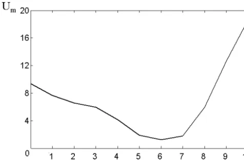
According to Eq. (3) the estimation error depends on the decomposition levelmand therefore there is an obvious need to find the decomposition levelm∗, which provides the small-est approximation error forfchar(t ).
Here we suggest a numerical stepwise algorithm for identi-fying the characteristic component of the geomagnetic signal model as outlined below.
1. The geomagnetic signalf0(t )is divided into segments of durationT, whereT is equal to 1 day (Nis the total number of discrete samples in the entire signal): {f0(tn)}Nn=1
={f0(tn)}Tn=1,{f0(tn)}2nT=T+1, . . ., {f0(tn)}Nn=N−T+1
.
2. The Sq curve and each segment of the geomagnetic signal are transformed into the wavelet domain using wavelet packets. The wavelet-packet transform is per-formed form= −1,−2, . . .,−J, whereJis determined by the segment lengthT:J≤log2T. Finally, we obtain the Sq curve components and each segment in the fol-lowing form:
f−mSq(t )=X n
cSq−m,nϕ−m,n(t ), f−ml (t )=X
n
cl−m,nϕ−m,n(t ),
wherelis the segment number.
3. The reconstruction of the components f−ml and f−mSq
is performed at each level m. Then the compo-nents are expressed as f0(−m),l(t )=P
n
c(−m),l0,n ϕ0,n(t ) andf0(−m),Sq(t )=P
n
c(−m),0,n Sqϕ0,n(t ), andU(−m),lis es-timated by applying expression Eq. (3):
U(−m),l= 1
T v u u t T X n=1 c (−m),l o,n −c
(−m),Sq 0,n 2 .
4. The decomposition levelm∗, which provides the lowest risk, is calculated as
er (−m∗)
=min −mmaxl U
Figure 3.Error of the characteristic variation estimationUmversus
the wavelet decomposition levelm.
5. The characteristic component of the geomagnetic signal is finally expressed as
f−m∗(t )=X n
c−m∗,nϕ−m∗,n(t ).
The resulting estimate can be improved by choosing the value forϕthat provides the lowest approximation error.
Using the data from the Paratunka observatory for 2002– 2008 and the algorithm above (steps 1–5), we calculated the estimation error of the characteristic field variation for vari-ous wavelet bases and decomposition levels. The goal was to find the optimal scalem∗that provided with the smallest ap-proximation error forfchar(t )(see Eq. 3). Figure 3 shows the error of the characteristic variation estimationUmversus the decomposition levelm. The figure indicates that for the cho-sen example, the smallest approximation error is obtained for the sixth decomposition level using the Daubechies wavelets (Daubechies, 2001) of the third order (see Fig. 3). Thus the reconstruction of the geomagnetic field variation component in the wavelet decomposition basis can be expressed as (see Eq. 1)
f (t )=fchar(t )+ X
jpert
gjpert(t )+e(t )
= X
n∈Z
c−6,nϕ−6,n(t ) !
+X
jpert
gjpert(t )+e(t ), (4)
wherec−6,n are the approximating coefficients of the sixth decomposition level for the wavelet packet decomposition,
ϕ−6,n is the basis function, and the component gjpert
deter-mines detailed coefficients containing perturbations. The in-dex set I includes the second, fourth, fifth, and sixth scale levels.
3.3 Extraction of the perturbed components of geomagnetic field variation
The degree of the geomagnetic signal disturbance is the so-called perturbation magnitude (Bartels et al., 1939), which can be assessed by calculating the difference between the greatest and the smallest deviations of the current field vari-ation from the characteristic diurnal varivari-ation, namely the Sq curve. In the suggested model (Eq. 1) the geomagnetic perturbations are characterized by the component
fpert(t )= X
jpert
gjpert(t ), (5)
where gjpert(t )=
P
n
djpert,n9jpert,n(t ), j ∈I are denoted as
jpert.
In order to identify the perturbed component of the geo-magnetic signal model, we next employ the wavelet-packet tree componentsgjpert(t ), which characterize the respective
perturbations. According to the results published earlier in Mandrikova et al. (2012, 2013b), the geomagnetic distur-bance Aj of the wavelet-packet tree component gj(t )= P
n
dj,n9j,n(t )can be determined as Aj=max
n dj,n
. (6)
Then the identification of these components is performed fol-lowing Rule 1:
j∈I, if mAvj> mAkj+εj, (7) wheremAvjis the sample average of the greatest wavelet coefficients (for scalej) for perturbed days,mAkj is the average of the greatest wavelet coefficients (for scalej )for quiet days,v is the index of the perturbed field variation,k
is the index of the quiet field variation, andεj determines a systematic shift between the perturbed and the quiet days.
AssumingAkj is normally distributed with meanµkj and varianceσjk, it is possible to estimateεjas
b
εj =x1−α/2
σjk
√
nk,
whereσjk is the variance of the greatest wavelet coefficients (for scalej) for quiet days (this variance is determined as a result of multiple measurements); x1−α/2 is the 1−α/2 quantile of the standard normal distribution;nk is the num-ber of analyzed quiet-field variations. Forα=0.1 the con-fidence probability is Pr=1−α/2=0.95, the quantile is
x1−α/2=1.96, andεj=1.96 σj √ n.
The scalesjpertare obtained from Eq. (7), correspond to the perturbed componentsgjpert of the model, and
Figure 4.Decomposition of the geomagnetic signal and its components in the period of a magnetic storm on 22–24 October 2016:(a)signal decomposition scheme, with perturbed components marked by the grey color;(b)H component of the Earth’s magnetic field, Paratunka observatory;(c)perturbed components of the geomagnetic field variations.
Figure 4 exemplifies the geomagnetic signal decomposi-tion for the observatory PET (Kamchatka) data, including the results of the extraction of perturbed components of the field variation by applying Rule 1 for the perturbed period during 22–24 October 2016. All decompositions included here and below were performed based on a third-order Daubechies wavelet determined by minimizing the approximation error (Mandrikova et al., 2012, 2013b). Signal components with perturbations are shown in the diagram in grey (Fig. 4a). The analysis of the results in Fig. 4b confirms the complex and nonstationary structure of a geomagnetic signal, which in-cludes multiscale components of the wide frequency band arising at random time points and characterizing periods of increased geomagnetic activity. One can see that, particu-larly prior to the magnetic storm, on 20–22 October the com-ponent g42 already contains short-term (instantaneous)
in-creases in the magnitude of the wavelet coefficients (Fig. 4c, indicated by dashed ellipses), which are possibly connected with instantaneous changes in the parameters of the inter-planetary environment (currents at magnetopause) (Gonzalez et al., 1999; Yermolaev and Yermolaev, 2010; Zaitsev et al., 2002). During the event, geomagnetic perturbations exhibit a wider spectrum and the magnitude of the wavelet coefficients increases drastically. Remarkably, a considerable growth in the geomagnetic perturbations on 22–24 October could also be observed, especially during the evening and night (18:00– 06:00 LT), which appeared to be more pronounced in the components g61 andgpert (see Fig. 4c) and is probably
as-sociated with current intensification in the tail of the
magne-tosphere (Gonzalez et al., 1999; Yermolaev and Yermolaev, 2010; Zaitsev et al., 2002).
3.4 Determining the quietest days and calculation of the Sq variation
In order to determine the characteristic diurnal variation, one has to identify the quietest diurnal variations for the an-alyzed time period and then calculate the average smoothed curve by averaging the variations over these days (usually the 5 quietest diurnal field variations within a period of 1 month are considered). The resulting curve determines the quiet-day diurnal variation in the geomagnetic field.
Identification of the quietest diurnal variations can be per-formed automatically by another suggested Rule 2:
if
A(j1)
pert=
1
L L X
n=1 d
(1) jpert,n
>
1
L L X
n=1 d
(2) jpert,n
=A
(2)
jpert, (8)
where L is the component length, then gj(1)
pert(t )=
L P
n=1
dj(1)
pert,n9jpert,n(t )for the scalejpertis more perturbed than
gj(2)
pert(t )=
L P
n=1
dj(2)
pert,n9jpert,n(t ). Then Ajpert=
1 L
L P
n=1 djpert,n
characterizes the degree of disturbance of the signal com-ponent for the scalejpert.
Figure 5.Quiet-day variations obtained in nonautomatic mode (red curve) and in the automatic mode (black curve):(a)Paratunka observa-tory;(b)Yakutsk observatory.
construct the average smoothed curve, namely the Sq curve, which is the zero baseline of theK index values (Bartels et al., 1939; Mandrikova et al., 2012, 2013b). Figure 5 indicates that by using Rule 2 the characteristic variations in the geo-magnetic field and the quiet-day diurnal variations can be re-constructed using the suggested wavelet-based technique in a fully automatic mode. In contrast to the suggested approach, existing techniques do not allow for the automatic perfor-mance of this operation. At present, we have performed the software implementation of this technique for Kamchatka (PET, IKIR RAS) and Yakutsk (YAK, IKFIA SD RAS), and the results of K index during its online calculation are presented at http://www.ikir.ru/en/Data/datalfg.html (last ac-cess: 30 August 2018) and http://ysn.ru/intermagnet/kindex (last access: 30 August 2018).
3.5 Extraction of weak and strong perturbations in the geomagnetic field
Let us consider three possible geomagnetic field activity lev-els:
1. activity levelh0 – the field is quiet (magnetic field is quiet);
2. activity levelh1 – the field is weakly disturbed (mag-netic field is weakly disturbed);
3. activity levelh2– the field is disturbed (magnetic field is disturbed).
According to these activity levels we can convert the math-ematical model Eq. (1) to the following form:
f (t )=fchar(t )+ X
(jpert,n)∈I1
djpert,n9jpert,n(t )
+ X
(jpert,n)∈I2
djpert,n9jpert,n(t )+e(t ), (9)
where
– fchar(t )is the characteristic component, – gpert,1(t )= P
(jpert,n)∈I1
djpert,n9jpert,n(t )is the component
characterizing weak geomagnetic perturbations, – gpert,2(t )= P
(jpert,n)∈I2
djpert,n9jpert,n(t )is the component
characterizing strong geomagnetic perturbations, – 9jpert=
9jpert,n n∈Zis the wavelet basis, – djpert,n=
f, 9jpert,n
are the wavelet coefficients, – jpertis the scale,
– nis the sample number, – I1, I2are the index sets, – e(t )is the noise.
Consider the following conditions ofdjpert,n for the
1. h0j
pert,n– the coefficient is quiet;
2. h1j
pert,n– the coefficient is weakly disturbed;
3. h2j
pert,n– the coefficient is disturbed.
The degree of the magnetic disturbance is deter-mined for its given magnitude by Eq. (6). To estimate
djpert,n (jpert,n)∈I 1 and
djpert,n (jpert,n)∈I
2 the threshold
func-tionsF1andF2are applied as follows:
f (t )=fchar(t )+ X
jpert,n
F1(djpert,n)9jpert,n(t )
+ X
jpert,n
F2(djpert,n)9jpert,n(t )+e(t ),
F1(x)=
0, if |x| ≤Tjpert,1 or |x|> Tjpert,2
x,ifTjpert,1<|x| ≤Tjpert,2
, (10)
F2(x)=
0,if |x| ≤Tjpert,2
x,if|x|> Tjpert,2
. (11)
The coefficients with the quiet condition h0j
pert,nare
consid-ered noise (they are equal to zero).
Both F1(x) and F2(x) determine the decision rules (Levin, 1963) for the condition of wavelet coefficients. Thresholds Tjpert,1 and Tjpert,2 split the coefficient space X
into three nonintersecting areas:X0, X1, X2.
In our case the decision rule is deterministic: if the given data set falls inXi, the hypothesis that a coefficient has con-ditionhij
pert,nis true. When a particular decision rule is used
for the conditionhij
pert,n, the average losses are
Ji(x)= 2 X
l=0
5ilP n
x∈Xl h
i jpert,n
o
, (12)
where5il is the loss function for erroneous decisions (each erroneous decision has its own cost),P
n x∈Xl
h
i jpert,n
o is the conditional probability of a data set falling in the area
Xl, if condition hijpert,n has occurred and i6=l, i, l are the condition indices.
The conditional average of the losses for the given con-dition hij
pert,n is known as the conditional risk.
Averag-ing the conditional risk function for each of the conditions
hij
pert,n, i=0,1,2 provides theaverage risk:
J∗= 2 X
l=0
piJi,
wherepi is the a priori probability of the conditionhijpert,n. The valueJ∗is the quality criterion for finding the deci-sion rule. The best rule is the one providing the lowest aver-age risk (known as the Bayesian risk; Levin, 1963).
Since the a priori distribution of the conditions is unavail-able, we will use the a posteriori risk to obtain thebest rule:
Jl(x)= 2 X
i=0
5ilP n
hij
pert,n|x∈Xl
o ,
where the a posteriori probabilitiesPnhij
pert,n|x
o
, i=0,1,2 provide the most complete characteristic of the conditions
hij
pert,nfor the given observational data. For the simple loss
function
5il=
5, i6=l,
0, i=l,
the a posteriori riskJl(x)equals Jl(x)=5
X
i6=l P
n hij
pert,n|x∈Xl
o
.
In this case the quality criterion for the decision rule is the smallest number of errors. The thresholdsTjpert,1andTjpert,2
are determined by the best decision rule, in particular the rule that provides the lowest value ofJl(x).
By minimizingJl(x)we estimated the thresholdsTj,1and
Tj,2j ∈I for the region of Kamchatka. The estimates were based on the geomagnetic data from the Paratunka station for the period between 2002 and 2008. The disturbance degree of the geomagnetic field was characterized by theKindex:
1. The coefficients belong to the areaX0(have thequiet conditionh0j
pert,n), if the current value of theKindex is
equal to 0 or 1.
2. The coefficients belong to the areaX1(have theweakly perturbed conditionh1j
pert,n), if the current value of the
Kindex is equal to 2, 3 or 4.
3. The coefficients belong to the area X2 (have the per-turbed condition h2j
pert,n), if the current value of the
Kindex is greater than 4.
Application of operations (9) and (10) allows one to auto-matically extract weak and strong perturbations characteriz-ing the activity level of the studied geomagnetic signal and thus to extract the information about the activity level of the geomagnetic field in the place of observation. The estimates have minute-scale time resolution, which allows one to ob-tain more detailed and prompt information about the activity of the geomagnetic field. It is also important that these trans-formations can be performed fully automatically.
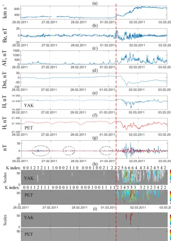
Figure 6. Data processing results for the period from 26 February 2011 to 2 March 2011:(a)speed of solar wind(b)Bz component of the interplanetary magnetic field;(c)AE index;(d)Dst index;(e)magnetic field variation for the Paratunka observatory;(f)magnetic field variation for the Yakutsk observatory;(g)identified perturbed components of the field variations (blue line – Yakutsk observatory, red line – Paratunka observatory);(h)results of applying operation 9 (above the plots we can seeKindices of the stations YAK and PET);(i)results of applying operation 10. The vertical dashed line indicates the onset of a magnetic storm.
Figure 6 also shows perturbed components of the geomag-netic field variations extracted using Rule 1 (Fig. 6g).
Prior to a magnetic storm the speed of solar wind did not exceed 400 km s−1, Bz component of the interplanetary mag-netic field (IMF) varied in the range of ±5 nT. The struc-ture of the obtained data components (Fig. 6g) indicates some general regularity of the geomagnetic field variations
from 00:50 to 01:30 UT) that are probably connected with the field of the current system of polar perturbations. By applying threshold functions (operations 9 and 10, Fig. 6h, i) one can confirm the appearance of weak perturbations in the geomagnetic field prior to the event at the high-latitude YAK station, while at the PET station (midlatitude), the ge-omagnetic activity did not exceed the corresponding thresh-old (Eq. 9). The values of K indices at the PET and YAK stations (Fig. 6h) also confirm a moderate increase in the ge-omagnetic activity at high latitudes. Furthermore, at the be-ginning of the day on 1 March (from 05:00 UT) the speed of solar wind started increasing and the component IMFBz con-tained oscillations±10 nT. Between 07:00 and 10:00 UT on 1 March the Dst index increased up to 20 nT, which confirms the outbreak of a magnetic storm (Gonzalez et al., 1999; Yer-molaev and YerYer-molaev, 2010; Zaitsev et al., 2002). At the an-alyzed stations YAK and PET, one could observe weak per-turbations (up to 10 nT, Fig. 6h). After 10:00 UT one could observe the onset of the main phase of a magnetic storm, which is characterized by a dramatic decrease in the Dst in-dex (to −88 nT). During the main phase of the storm on 1 March from 09:10 to 15:45 UT, from 17:00 to 18:45 UT, from 19:45 to 20:45 UT one could see a dramatic rise of AE indices (to 1350 nT), which confirms strong substorms in the auroral area. An analysis of the perturbed components of the geomagnetic field variations (Fig. 6g) shows clear cor-relations between the periods of increase in AE indices and significant short-term increases in the geomagnetic activity at the YAK station (characterized by the abrupt peaks of high magnitude in the perturbed component) mostly during night-time (from 21:00 to 06:00 LT) that could probably be associ-ated with auroral processes and the intensification of currents in the magnetosphere’s tail. The results of applying thresh-old functions (operation 10, Fig. 6i) confirm a significant increase in the activity at the YAK station during the main phase of the storm (1 March from 22:10 to 02:50 LT). At the midlatitude station PET, perturbations were rather moderate (did not exceed the thresholdsTjpert,2, Fig. 6i) and exhibited
activity on the low-frequency spectrum, which allows us to attribute them to the intensification of the ring current during the main phase of the storm (Gonzalez et al., 1999; Yermo-laev and YermoYermo-laev, 2010; Zaitsev et al., 2002). The recovery phase lasted for several days and was followed by continuous auroral activity (Fig. 6c) and weak perturbations in the field at the PET and YAK stations, which is typical (Gonzalez et al., 1999) of a storm caused by the high-speed flow of a coro-nal hole.
3.6 Extraction and estimation of nonstationary short-term variations in the geomagnetic field
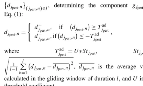
Due to the continuous variability of magnetospheric pro-cesses, especially during perturbed periods, we can in-troduce the adaptive thresholds Tjad
pert and the coefficients
djpert,n (jpert,n)∈I, determining the component gjpert in
Eq. (1):
djpert,n=
( dj+
pert,n, if djpert,n
≥Tjad
pert
dj−
pert,n,if djpert,n
≤ −Tjad
pert
, (13)
where Tjad
pert=U∗Stjpert, Stjpert=
s 1 l−1 l P k=1
djpert,n−djpert,n
2
, djpert,n is the average value
calculated in the gliding window of durationl, andU is the threshold coefficient.
Then following Eq. (6) the intensity of positive (I+) and negative (I−) perturbations in the geomagnetic field at the time pointt=ncan be determined as
In+−=X jpert
d
+− jpert,n
[image:11.612.309.547.63.207.2]
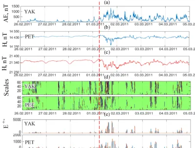
. (14)
Figure 7 shows the results of applying operations (12) and (13) with the following parameters: coefficient U=2 and window lengthl=720samples (corresponding to 12 h), Fig. 7d, e during the event on 1 March 2011 (the event is described above, see Fig. 6 and the description in Sect. 3.5). The analysis of the results in Fig. 7 confirms the efficacy of the adaptive thresholding Eq. (12) and shows that this al-lowed for the extraction of nonstationary short-term changes in data characterizing the appearance of weak increases in geomagnetic activity at the YAK and PET stations that pre-ceded a major magnetic storm. The extracted perturbations could be observed nearly synchronously at the PET and YAK stations, correlated with the increase in the AE in-dex, and were probably associated with short-term (instanta-neous) changes in the parameters of the interplanetary envi-ronment (Gonzalez et al., 1999; Yermolaev and Yermolaev, 2010; Zaitsev et al., 2002). During the initial phase of the storm the intensity of the geomagnetic perturbations at the analyzed stations increased drastically (see Fig. 7e). During the main phase of the storm we also observed short-term dra-matic increases in the intensity of the geomagnetic perturba-tions (see Fig. 7e). Thus, the application of Eqs. (12) and (13) allowed us to extract and estimate nonstationary (within the analyzed window of durationl) short-term increases in the geomagnetic activity, which provide a more in-depth view of the dynamics of geomagnetic processes.
4 Experimental results and discussion
Figure 7.Data processing results for the period from 26 February 2011 to 4 March 2011:(a)AE index;(b)magnetic field variation for the Paratunka observatory;(c)– magnetic field variation for the Yakutsk observatory;(d)results of applying adaptive thresholds Eq. (12), the red color indicates positive perturbations (increases relative to trend), the blue color shows negative ones (decreases relative to trend); (e)results of applying operation (13), the red color indicates positive perturbations (increases relative to trend), the blue color shows negative ones (decreases relative to trend). The vertical line indicates the onset of a magnetic storm.
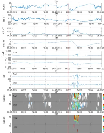
ejection (CME; the catalogue of ICMES by Ian Richard-son and Hilary Cane, http://www.srl.caltech.edu/ACE/ASC/ DATA/level3/icmetable2.htm) that occurred 3 days before exhibiting the typical phases of the Dst variation (Gonza-lez et al., 1999; Yermolaev and Yermolaev, 2010; Zaitsev et al., 2002). Prior to the storm the speed of solar wind was greater than average (> 400 km s−1) (Gonzalez et al., 1999; Yermolaev and Yermolaev, 2010; Zaitsev et al., 2002) and the Bz component experienced a change of±11 nT. Figure 8 shows that on 6 January, prior to the event, the increase on the AE index (Fig. 8c) at the analyzed stations was accom-panied by weak perturbations in the geomagnetic field (see Fig. 8g, calculated by Eq. 9): at 07:00–11:00 UT, 16:00– 18:30 and 19:20–21:10 UT at the YAK stations, at 8:00– 11:00 and 17:00–21:10 UT at the PET stations. These results are in accordance with those of Davis (1997) and Zhang and Moldwin (2015), where prior to magnetic storms, one can observe characteristic increases in solar wind parameters and the power of IMF followed by increases in the geomagnetic activity indices (AE, Kp). The coincidence of the periods of increased geomagnetic activity at the analyzed stations with
the periods in the AE index increases following fluctuations in the Bz component (Fig. 8a), allowing us to suggest the connection of the extracted geomagnetic perturbations with the nonstationary changes in the parameters of the interplan-etary environment and the intensification of auroral activity (Gonzalez et al., 1999; Yermolaev and Yermolaev, 2010; Za-itsev et al., 2002). At the beginning of the day on 7 January, the Bz component turned to the south (at 00:20 UT) and in this period decreased to the value of−5 nT at both the YAK and PET stations. At the same time, short-term perturbations (from 01:15 to 01:30 UT, Fig. 8g) could be observed. Also, at the initial phase of the storm, increases in the Dst index (from 06:00 UT) and in auroral activity (see Fig. 8c) could be observed, accompanied by weak perturbations in the geo-magnetic field at both the YAK and PET stations (Fig. 8g).
Figure 8.Processing results of the data for 6–8 January 2015;(a)Bz component of the interplanetary magnetic field;(b)speed of solar wind; (c)AE index;(d)Dst index;(e)H component of the magnetic field;(f)identified perturbed components of the geomagnetic field variations; (g)results of applying threshold function (9);(h)results of applying threshold function (10). The vertical dashed line indicates the onset of a magnetic storm.
the geomagnetic longitude) is located in the midlatitude area. Figure 8f, g, h show that the increase in the geomagnetic per-turbations and the moments of extrema (where perper-turbations reached 175 nT at the YAK station while they reached 50 nT at the PET station) occurred at the stations at the same time, mostly during nighttime or evening hours.
An application of Eqs. (12) and (13) to the data from a net-work of meridionally located stations (from high latitudes to the Equator) shows the distribution of the perturbations along the meridian of observations and confirms the general dy-namics of nonstationary short-term perturbations in the
geo-magnetic field prior to a geo-magnetic storm and during the event (see Fig. 9e). Quantitative estimates (by Eq. 13, Fig. 9e) show significant correlations of the extracted geomagnetic pertur-bations with the AE index, not only in their occurrence times, but also in their intensities.
Figure 9.Processing results of the data for 6–8 January 2015;(a)Bz component of the interplanetary magnetic field;(b)speed of solar wind; (c)AE index;(d)Dst index;(e)calculations following Eq. (13). Red color indicates positive perturbations (relative to trend), blue indicates negative (relative to trend). The vertical dashed line indicates the onset of a magnetic storm.
circle: 7 January from 00:50 to 01:45 UT) were visible. This confirms the connection of the extracted perturbations with the auroral processes and also with the increase in the netosphere’s tail currents during the main phase of a mag-netic storm. Possible connections of the ring current with the processes in the auroral area are provided in Mendes et al. (2005). The reconstruction phase was short, at 20:00 UT the Dst index increased to−35 nT, which is common for the events from a CME (Gonzalez et al., 1999). At the end of the day on 7 January, fluctuations in the Bz component of the interplanetary magnetic field (±10 nT, Fig. 8a) accompanied by the fluctuations of the speed of solar wind (Fig. 8b) and followed by weak perturbations in the geomagnetic field at both YAK and PET stations (see Fig. 8g) as well as at the equatorial station GUA (see Fig. 9e) could be observed.
Figure 10 shows similar results obtained during the mag-netic storm on 17 March 2015. This event is character-ized as a “double storm” (magnetic storm with two main phases) and is caused by two separate emissions of the solar substance (the catalogue of ICMES by Ian Richard-son and Hilary Cane, http://www.srl.caltech.edu/ACE/ASC/ DATA/level3/icmetable2.htm). Prior to a magnetic storm
Figure 10.Processing results for observations on 15–18 March 2015;(a)Bz component of the interplanetary magnetic field;(b)speed of solar wind;(c)AE index;(d)Dst index;(e)H component of the magnetic field;(f)identified perturbed components of the geomagnetic field variations;(g)results of applying the threshold function (9);(h)results of applying the threshold function (10). The vertical dashed line indicates the onset of a magnetic storm.
Moldwin (2015). At 04:00 UT on 17 March, due to the ar-rival of solar mass from CME (the catalogue of ICMES by Ian Richardson and Hilary Cane, http://www.srl.caltech. edu/ACE/ASC/DATA/level3/icmetable2.htm), the speed of solar wind reached 510 km s−1while the Bz component of the interplanetary magnetic field reached 26 nT. In 45 min (at 04:00 UT) at the PET station, the onset of a magnetic storm was registered. At the YAK station the initial phase of the storm was less noticeable (Fig. 10e–g). The strongest geomagnetic perturbations at this station began occurring 08:50 UT (Fig. 10h), with their magnitude reaching 307 nT,
(Fig. 10f). This was accompanied by the reduction in the Dst index in this period to−77 nT, and the AE index reaching 1055 nT.
by a strong decrease in the Dst index (to−224 nT). During this period there were strong substorms in the auroral area, where the AE index reached a maximal value of−2250 nT (see Fig. 10c). A detailed analysis of the event based on the application of Eqs. (12) and (13) (see Fig. 11f) indicates that at the beginning of a magnetic storm, at all analyzed stations (from those located at high latitudes to the Equator), one could notice a short-term increase in the geomagnetic activ-ity. During the fluctuations of the Bz component of the inter-planetary magnetic field (to±23 nT, Fig. 11a) and during an increase in the AE index (from 06:00 to 09:00 UT, Fig. 11c), strong short-term perturbations were observed, mostly at the stations closer to the north, particularly YAK, PET, and MGD (see Fig. 11f). After the arrival of high-speed flows of so-lar mass from the second CME on 17 March from 12:35 to 15:15 UT, one could observe a significant increase in the AE index (Fig. 11c), a decrease in the Dst index (Fig. 11d), and strong short-term perturbations in the geomagnetic field at all analyzed stations (Fig. 11f). An analysis of perturbed com-ponents of the field variations (Fig. 11e) and a comparison of the results with the results of Eqs. (12) and (13) (Fig. 11f) show that during the time of the greatest decrease in the Dst index (Fig. 11d) at low-latitude stations KHB and GUA, there were strong geomagnetic low-frequency spectrum per-turbations (fluctuations with the period from 20 to 50 min, see Fig. 11e), which likely indicate their connection with the strong intensification of the ring current during the second main phase of a magnetic storm.
Our results indicate the complex dynamics of the spa-tiotemporal distribution of geomagnetic perturbations dur-ing the periods of increased solar activity and magnetic storms. A detailed analysis of the events on 7 January and 17 March 2015 confirmed the occurrence of weak short-term perturbations in the geomagnetic field prior to mag-netic storms. The extracted perturbations were observed at all analyzed stations (from those located at high latitudes to the Equator), exhibited nonstationary behavior, and were ac-companied by the fluctuations of the Bz component of the interplanetary magnetic field and increase in the AE index. These results are in accordance with those of Davis (1997) and Zhang and Moldwin (2015), which allows us to suggest their external nature and connection with the nonstationary impact of solar wind on the Earth’s magnetosphere. In Davis (1997) and Zhang and Moldwin (2015), it has been shown that increases in solar wind parameters and the subsequent increases in geomagnetic activity (AE, Kp indices) can be observed prior to the abrupt turns of the IMF towards the south, then leading to magnetic storms (Lockwood, 2016).
The analysis of the results of this work also showed cor-relations of the occurring geomagnetic perturbations with the AE index not only in their occurrence times but also in their intensities. One possibility of extracting such abnor-mal effects as a result of processing ground-based geomag-netic data has also been suggested in Barkhatovetal (2016) and Sheiner and Fridman (2012) and was mentioned briefly
in Mandrikova et al. (2013a). The analyses of the authors Barkhatov et al. (2016) and Sheiner and Fridman (2012), based on observational data and the joint analysis of the oscillations of the H component of the geomagnetic field with the oscillating processes on the Sun, have shown that the probability of these abnormal effects is high and reaches nearly 90 %. Here we have confirmed this effect using a very different approach and have shown explicitly that the suggested technique can successfully extract corresponding events. An analysis of the variations in the Dst index in the periods preceding magnetic storms can be found in Balasis et al. (2006), where we can also find the assumption that the critical feature of persistence in the magnetosphere is the re-sult of combining solar wind with the internal magnetosphere activity (the magnetosphere is affected by solar wind).
Accordingly, an important aspect of this approach is the possibility of extracting prestorm anomalies based on the analysis of the ground-based data and the possibility of the automatic implementation of the technique, with online per-formance exhibiting only minor delays. Several hours prior to the analyzed magnetic storms, weak variations in the inter-planetary magnetic field (±5 nT for 7 January and±6 nT for 17 March) were accompanied by a moderate increase in the AE index (to 150 nT on 7 January and 117 nT on 17 March) and a moderate increase in the geomagnetic activity at the equatorial station GUA. During the main phases of the an-alyzed magnetic storms the geomagnetic perturbations in-creased drastically, exhibiting a nonstationary spectrum de-pending on the station where the data were measured, which could be attributed to the complex dynamics of the current system during magnetic storms (Gonzalez et al., 1999; Yer-molaev and YerYer-molaev, 2010; Zaitsev et al., 2002).
5 Conclusions
To summarize, we have suggested, implemented, and val-idated a mathematical model and automated algorithms to analyze and describe the geomagnetic field variations based on the wavelet-based multiscale approach. Our results indi-cate that the model is particularly capable of reflecting the characteristic variation and local perturbations in the geo-magnetic field during periods of increased geogeo-magnetic ac-tivity. The efficiency of applying the wavelet transform in the analysis of geomagnetic data and the study of nonstation-ary processes in the magnetosphere can also be found in the works of other authors (e.g., Mendes et al., 2005; Hafez et al., 2013). In our research, we have suggested Rule 1 (oper-ation 7) for identifying components containing geomagnetic perturbations. The magnitudes of the components extracted using Eq. (7) allow us to estimate the degree of geomagnetic activity.
Figure 11.Processing results for observations on 15–18 March 2015;(a)Bz component of the interplanetary magnetic field;(b)speed of solar wind;(c)AE index;(d)Dst index;(e)identified perturbed components of the field variations;(f)results of applying Eq. (13), red color indicates positive perturbations (increases relative to trend), blue indicates negative (decreases relative to trend). The vertical dashed line indicates the onset of a magnetic storm.
et al., 2005) together with the wavelet transform. In our work, we have suggested the technique of threshold estimation, and these thresholds allow us to extract geomagnetic perturba-tions in varying intensities (see Eqs. 9 and 10). We have also considered the adaptive threshold (see Eq. 12) for a more detailed analysis of the dynamics of the process. Analyses of moderate magnetic storms on 1 March 2011 and 7 Jan-uary 2015 and of strong magnetic storms on 17 March 2015 have shown the efficiency of the suggested solutions.
Our experimental results clearly indicate the high sensitiv-ity of the suggested technique and the possibilsensitiv-ity of its appli-cation in the in-depth study of the dynamics and spatiotem-poral distribution of the geomagnetic perturbations (based on
Data availability. Geomagnetic data from the stations of the Insti-tute of Cosmophysical Research and Radio Wave Propagation are available at the following link: http://www.ikir.ru:8180 (Institute of Cosmophysical Research and Radio Wave Propagation FEB RAS, last access: 30 August 2018). Data from other stations are avail-able to everyone (http://intermagnet.org; Intermagnet, last access: 30 August 2018). The algorithms used in the paper are provided in Sect. 3.4–3.6 and the values of the parameters of the threshold functions are given in Sect. 3.6.
Author contributions. OVM has developed the model and helped develop the algorithm, performed a detailed analysis of the process-ing results and prepared the manuscript. ISS has performed the es-timation of model parameters, developed and implemented the al-gorithms, performed data processing and prepared the manuscript. SYK has performed primary data processing and helped analyze and edit the manuscript. VVG helped develop the model. DMK helped to analyze and edit the manuscript. MIB helped to analyze and edit the manuscript. All the authors took part in analyzing and discussing the results.
Competing interests. The authors declare that they have no conflict of interest.
Acknowledgements. The research is supported by the grant of the Russian Science Foundation (project no. 14-11-00194). We would like to thank the staff of the geomagnetic observatories at IKIR FEB RAS and at IKFIA SB RAS for providing high-quality exper-imental data. The results presented in this paper rely on the data collected at the Guam observatory. We thank USGS for supporting its operation and INTERMAGNET for promoting high standards of magnetic observatory practice (http://www.intermagnet.org; last access: 30 August 2018).
The topical editor, Georgios Balasis, thanks two anony-mous referees for help in evaluating this paper.
References
Balasis, G., Daglis, I. A., Kapiris, P., Mandea, M., Vassiliadis, D., and Eftaxias, K.: From pre-storm activity to magnetic storms: a transition described in terms of fractal dynamics, Ann. Geo-phys., 24, 3557–3567, https://doi.org/10.5194/angeo-24-3557-2006, 2006.
Balasis, G., Daglis, I. A., Zesta, E., Papadimitriou, C., Georgiou, M., Haag-mans, R., and Tsinganos, K.: ULF wave activity dur-ing the 2003 Halloween superstorm: multipoint observations from CHAMP, Cluster and Geotail missions, Ann. Geophys., 30, 1751–1768, https://doi.org/10.5194/angeo-30-1751-2012, 2012. Balasis, G., Daglis, I. A., Georgiou, M., Papadimitriou, C., and Haagmans, R.: Magnetospheric ULF wave studies in the frame of Swarm mission: a time-frequency analysis tool for automated de-tection of pulsations in magnetic and electric field observations, Earth Planet. Space, 65, 1385–1398, 2013.
Balasis, G., Papadimitriou, C., Daglis, I. A., and Pilipenko, V.: ULF wave power features in the topside ionosphere revealed by Swarm observations, Geophys. Res. Lett., 42, 6922–6930, https://doi.org/10.1002/2015GL065424, 2015.
Barkhatov, N. A., Obridko, V. N., Revunov, S. E., Snegirev, S. D., Shadrukov, D. V., and Sheiner, O. A.: Long-period geomagnetic pulsations as solar flare precursors, Geomagn. Aeron., 56, 265– 272, 2016.
Bartels, J., Heck, N. H., and Johnson, H. F.: The three-hour-range index measuring geomagnetic activity, Terrestrial Magnetism and Atmospheric Electricity, 44, 411–454, 1939.
Berryman, J. G.: Choice of operator length for maximum entropy spectral analysis, Geophysics, 43, 1384–1391, 1978.
Chen, G. X., Xu, W. Y., Du, A. M., Wu, Y. Y., Chen, B., and Liu, X. C.: Statistical characteristics of the day-to-day vari-ability in the geomagnetic Sq field, J. Geophys. Res., 112, https://doi.org/10.1029/2006JA012059, 2007.
Consolini, G., De Marco, R., and De Michelis, P.: Intermittency and multifractional Brownian character of geomagnetic time series, Nonlin. Proc. Geophys., 20, 455–466, 2013.
Daubechies, I.: Ten Lectures on Wavelets, Society for Industrial and Applied Mathematics, 2001.
Davis, C. J., Wild, M. N., Lockwood, M., and Tulunay, Y. K.: Ionospheric and geomagnetic responses to changes in IMF BZ: a superposed epoch study, Ann. Geophys., 15, 217–230,
https://doi.org/10.1007/s00585-997-0217-9, 1997.
Davis, T. N. and Sugiura, M.: Auroral electrojet activity index AE, J. Geophys. Res., 71, 785–801, 1966
Golovkov, V. P., Papitashvili, V. O., and Papitashvili, N. E.: Auto-mated calculation of theKindices using the method of natural orthogonal components, Geomagn. Aeron., 29, 667–670, 1989. Gonzalez, W. D., Tsurutani, B. T., and Clua-Gonzalez, A. L.:
In-terplanetary origin of geomagnetic storms, Space Sci. Rev., 88, 529–562, 1999.
Hafez, A. G., Khan, T. A., and Kohda, T.: Clear P-wave arrival of weak events and automatic onset determination using wavelet fil-ter banks, Digital Signal Processing, 20, 715–723, 2010. Holschneider, M.: Wavelets: an Analysis Tool, Clarendon, Oxford,
England, 1995.
Jach, A., Kokoszka, P., Sojka, J., and Zhu, L.: Wavelet-based in-dex of magnetic storm activity, J. Geophys. Res., 111, a09215, https://doi.org/10.1029/2006ja011635, 2006.
Joselyn, J. A.: A real-time index of geomagnetic activity, J. Geo-phys. Res., 75, 2777–2780, 1970.
Klausner, V., Papa, A. R. R., Mendes, O., Domingues, M. O., and Frick, P.: Characteristics of solar diurnal variations: A case study based on records from the ground magnetic station at Vassouras, Brazil, J. Atmos. Sol.-Terr. Phys., 92, 124–136, 2013.
Kovacs, P., Carbone, V., and Vörös, Z.: Wavelet based filtering events from geomagnetic time-series, Planet. Space Sci., 49, 1219–1231, 2001.
Kumar, P. and Foufoula-Georgiou, E.: Wavelet analysis for geo-physical applications, Rev. Geophys., 35, 385–412, 1997. Kunagu, P., Balasis, G., Lesur, V., Chandrasekhar, E., and
Levin, B. R.: Theoretical Basis of Statistical Radio Techniques, Fiz-matgiz, Moscow, 1963.
Lockwood, M., Owens, M. J., Barnard, L. A., Bentley, S., Scott, C. J., and Watt, C. E.: On the origins and timescales of geoeffective IMF, Space Weather, 14, 406–432, https://doi.org/10.1002/2016SW001375, 2016.
Lovejoy, S., Pecknold, S., and Schertzer, D.: Stratified multifractal magnetization and surface geomagnetic fields – I. Spectral anal-ysis and modeling, Geophys. J. Int., 145, 112–126, 2001. Mandrikova, O. V., Solovjev, I. S., Geppener, V. V., and Klionskiy,
D. M.: New wavelet-based approach intended for the analysis of subtle features of complex natural signals, S. Mach. Perc., 21, 293–296, 2011.
Mallat, S.: A Wavelet tour of signal processing, Academic Press, 1999.
Mandrikova, O. V., Smirnov, S. E., and Solov’ev, I. S.: Method for Determining the Geomagnetic Activity Index Based on Wavelet Packets, Geomagn. Aeron., 52, 111–120, 2012.
Mandrikova, O. V., Bogdanov, V. V., and Solovjev, I. S.: Wavelet Analysis of Geomagnetic Field Data, Geomagn. Aeron., 53, 268–276, 2013a.
Mandrikova, O. V., Solovjev, I., Geppener, V., Taha Al-Kasasbehd R., and Klionskiy, D.: Analysis of the Earth’s magnetic field vari-ations on the basis of a wavelet-based approach, Digital Signal Processing, 23, 329–339, 2013b.
Mandrikova, O. V., Solovev, I. S., and Zalyaev, T. L.: Meth-ods of analysis of geomagnetic field variations and cosmic ray data, Earth Planet. Space, 66, https://doi.org/0.1186/s40623-015-0228-9, 2014.
Mendes, O. J., Oliveira, M. D., Mendes da Costa, A., and Clùa de Gonzalez, A. L.: Wavelet analysis applied to magnetograms: Sin-gularity detections related to geomagnetic storms, J. Atmos. Sol.-Terr. Phys., 67, 1827–1836, 2005.
Menvielle, M., Papitashvili, N., Hakkinen, L., and Sucksdorff, C.: Computer production of K indices: review and comparison of methods, Geophys. J. Int., 123, 866–886, 1995.
Nayar, S. R. P., Radhika, V. N., and Seena, P. T.: Investigation of substorms during geomagnetic storms using wavelet Techniques, ILWS WORKSHOP, GOA, India, 9–24, 2006.
Nowo˙zy´nski, K., Ernst, T., and Jankowski, J.: Adaptive smoothing method for computer derivation of K-indices, Geophys. J. Int., 104, 85–93, 1991.
Pecknold, S., Lovejoy, S., and Schertzer, D.: Stratified multifractal magnetization and surface geomagnetic fields – II. Multifractal analysis and simulations, Geophys. J. Int., 145, 127–144, 2001. Rangarajan, G. K.: Indices of geomagnetic activity, in:
Geomag-netism, edited by: Jacobs, J. A., vol. 3, Academic Press, London, 323–384, 1989.
Rotanova, N., Bondar, T., and Ivanov, V.: Wavelet Analysis of Sec-ular Geomagnetic Variations, Geomagn. Aeron., 44, 252–258, 2004.
Sheiner, O. A. and Fridman, V. M.: The features of microwave solar radiation observed in the stage of formation and initial propaga-tion of geoeffective coronal mass ejecpropaga-tions, Radiophys. Quantum El., 54, 655–666, 2012.
Sucksdorff, C., Pirjola, R., and Häkkinen, L.: Computer production of K-values based on linear elimination, Geophys. Trans., 36, 333–345, 1991.
Sugiura, M.: Hourly values of equatorial Dst for the IGY, Ann. Int. Geophys. Year, 35, p. 44, 1964.
Thebault, E., Finlay, C. C., Beggan, C. D. et al.: International Ge-omagnetic Reference Field: the 12th generation, Earth Planet. Space, 35, 9–45, 1964.
Xu, Z., Zhu, L., Sojka, J., Kokoszka, P., and Jach, A.: An assess-ment study of the wavelet-based index of magnetic storm activity (WISA) and its comparison to the Dst index, J. Atmos. Sol.-Terr. Phys., 70, 1579–1588, 2008.
Yermolaev, Yu. I. and Yermolaev, M. Yu.: Solar and
In-terplanetary Sources of Geomagnetic Storms: Space
Weather Aspects, Izv. Atmo. Ocean. Phy., 46, 799–819, https://doi.org/10.1134/S0001433810070017, 2010.
Zaitsev, A. N., Dalin, P. A., and Zastenker, G. N.: Sudden variations in the solar wind ion flux and their signature in the geomagnetic field disturbances, Geomagn. Aeron., 42, 717–724, 2002. Zaourar, N., Hamoudi, M., Mandea, M., Balasis, G., and
Holschneider, M.: Wavelet-Based Multiscale Analysis of Ge-omagnetic Disturbance, Earth Planet. Space, 65, 1525–1540, https://doi.org/10.5047/eps.2013.05.001, 2013.