Abstract: In the point of large big data and massive increase the rate of time series data flow in the upcoming market program business, mining of related data and real time data[1] are been briefly explained. This paper proposes predicted the value of the trader marketing when we reach the expected the value and increase the rate of accuracy. For this purpose we can use the time series algorithm in machine learning and gets regular item sets by using the corresponding of Map reduce [2], which consumes less space and will not increase the time overhead. The usage of CPU is improved by using the thread calling algorithm and batch algorithm, it meets deep business opportunities and requirement processing or feature model based on the requirements of traders. Thus our results indicates that the model not only explained the time series data stream[4],it also helps traders to get to a confirmation that they can achieve data quickly and achieve accuracy trade off's. This paper proposes a new demand forecasting model which is an extension of the traditional exponential diffusion models [5]. We examined the forecasting performance of the models just after the release of the item when the small number of model calibration data is available. This paper shows that the model which we proposed has the thing of enabling early decision making and best performance.
Keywords: Time Series Data, Machine Learning, Map Reduce, Diffusion Models.
I. INTRODUCTION
In recent years, with the non-discrete expansion of the next generation market programs and the gradual increase of the investment type of concept in some countries, a massive [6] type of time series data that to be processed has been created in the transaction, that are entirely different from compared to the traditional data and the present techniques of very large amount of data, the execution speed and the generation rate increased time. Such that with the less processor and memory resources, ensure of the time series data can be executed/processed effectively and is becoming more and more important and effective. Most of the scholars focus on the real-time and effective data mining and processing association rules, then will be having much academic based research. The processes of literature of big data through the distributed parallel[7] type of calculation, and then it proves that decreasing the late process of the data
Revised Manuscript Received on July 22, 2019.
N.Deepa, Assistant Professor, Saveetha School of Engineering, SIMATS, Chennai
M. Bhuvanachandra, UG Student, Saveetha School of Engineering, SIMATS, Chennai
B. Reddyprasad, UG Student, Saveetha School of Engineering, SIMATS, Chennai
M.Nagendra, UG Student, Saveetha School of Engineering, SIMATS, Chennai
transmission can effectively reduce the impact of late process of the processing the results. The proposed system of literature says that the permanent memory of the data can be use the disk Input Output overhead and increases the rate of data that is for accessing. On the basis of the new data structure, it increases the effectiveness of finding the most frequent item sets using Hah table storage type of technology and the usage or the optimization of the Apriori[8] algorithm. The next literature improves/increases the traditional usage of Apriori algorithm using the MapReduce in parallel, but these increments are only consider to the number of steps, creating a massive number of candidate sets or seeking to scan the database n number times. When the data is very massive, it will generate a very huge candidate set greatly decreasing the efficiency of the algorithm. On the another hand, the distributed program model based on the RTMR[9] method provides us very massive data storage and parallel computing real-timely[10], it makes very full use of the resource and optimizes the CPU utilization, thus provides the better process and data processing model.
II. DEMAND FORECASTING OF NEW ITEMS
Forecasting the new items in shopping media a number of researchers under science area marketing can develop several methods. One of the major and main forecast new items researcher is the development of predicting the forecast method value. Another side of the development is increasing the accuracy of the predicted value when compare with the excepted value.
Prediction for forecasting methods
For the purpose of prediction of forecasting methods utilize the available test data in market. In that market test data can having the sub headers has region, post-Shipment Invoice Date, Customer Code, Technology, SAP Item Code, Qty(Net), SO Date, End Customer Code and plant. Initially the region can access the post shipment data for the shipping date for the user in market for increase their profits. After gave the post shipment date, provider can access the customer information about address for delivery their product in the market. For this purpose, the service provider can discovery the code called Customer code. Customer Code can have all type of data where the customer personal data to customer ordered data. And the third party of this forecast shipment is by where this process can be done by the way of execution. That execution can do by the step by step process.
Predict the Shipment Forecast using
Time-Series Data in Machine Learning
By doing this all process called as Technology. SAP Item Code can having the data sku vce number where the product can order and which can product can be placed as well as delivery also. SO Date can having the dates where the customer can took their delivery product.
Region
Region can be allocated by the different places on the map in British rule for trading as shown in the figure.
Region
[image:2.595.377.472.128.624.2]reg_1
reg_2
reg_3
reg_3
reg_4
Fig. 2.1.1
Fig.2.1.2 Post-Shipment Invoice Date
Post-Shipment Invoice Date is the date where the customer can order the data for product as shown in the figure.
Customer Code
Customer Code is the identity for the customer order and product reference as shown in the figure.
Fig. 2.1.3
III. SYSTEM IMPLEMENTATION
Front-end process
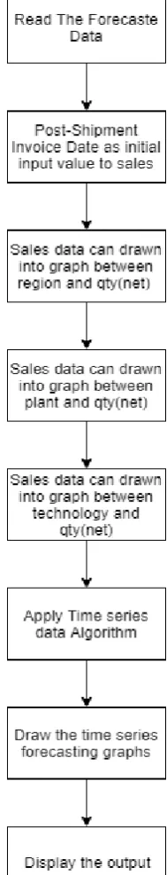
This Front end process can do step by step. Initially, we can read the forecast data for defining the output. After we can take the post-shipment invoice date as initial input values to sales. Then draw the graphs between the region and qty(net) by using the dataframes name as sales. Then after draw the graphs between the plant and qty(net) by
using the dataframes name as sales1. Again draw the graphs between the technology and qty(net) by using the dataframes name as sales2. Apply the Time Series data algorithm to the data. Then draw the times series forecasting graphs. Finally shown the output and the process can do by step by step as shown in the figure.
Fig. 3.1.1Front end system architecture Back-End Process
This Back-End process can done step by step. Initially, we can import the data from the device where the market time data can be stored. And then we can read the data for defining the output.
Post-Shipment Invoice Date
08-12-2015
08-12-2015
23-11-2015
10-12-2015
03-12-2015
Customer Code
[image:2.595.47.269.162.431.2]After we can creates the dataframes for the coding whose dataframe name called as sales. Then draw the graphs between the region vsqty(net) by using the dataframes name as sales and plant vsqty(net) by using the dataframes name as sales1and technology vsqty(net) by using the dataframes
[image:3.595.58.546.124.586.2]name as sales2. Apply the Time Series data algorithm to the dataframes (sales). Then predict the value by using the algorithm. Finally compare the value with the excepted value. This process can done as shown in the figure.
Fig. 3.2.2 Back End process
IV. EXECUTION AND RESULT Process of the execution
Read the data
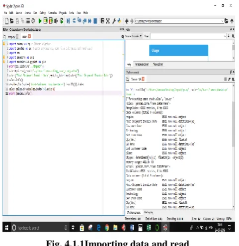
For reading the data we can first import the data and then read as shown in the figure.
Fig. 4.1.1Importing data and read Graph between region vsqty(net)
[image:3.595.310.543.310.566.2]For the drawn the graph we can create the dataframes and run the code as shown in the figure:
Fig. 4.1.2Creating Data Frames and running the code regionvsqty(net)
Graph between plant vsqty(net)
[image:3.595.50.291.420.668.2]Fig. 4.1.3 plant vsqty(net) Graph between technology vsqty(net)
[image:4.595.325.514.110.250.2]For the drawn the graph we can create the dataframes and run the code as shown in the figure:
Fig. 4.1.4 Technology vsqty(net) Plots between date, year, month vsqty(net)
For the drawn the plots between the date, year, month vsqty(net) we can access the dataframes and divided into subplots as shown in the figure.
Fig. 4.1.5Date, year, month vsqty(net)
Plot between Final-date vsqty(net)
[image:4.595.49.291.314.531.2]When plotting the graph between the final date vsqty(net) we can consider the dataframes where the order can be placed as shown in the figure.
Fig. 4.1.6 Final-date vsqty(net) Decomposition of Plots
[image:4.595.307.548.330.496.2]Purpose of decomposition of the plots is analysis where and when net can be raised or dropped.
Fig. 4.1.7 Analysing the subplots in each stage
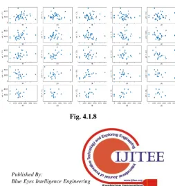
Purpose of this subplots can be expose the each and every sub connecting between the various sub headers as shown in the figure.
[image:4.595.306.560.554.825.2] [image:4.595.55.284.594.768.2]Predict and expected values
Fig. 4.1.9
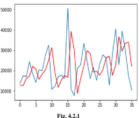
4.2 Graph between predict and expected value
[image:5.595.357.497.316.489.2]Accuracy percentage between predict and expected value
Fig. 4.2.1
Each and every stage accuracy percentage can be raised as shown in the table.
Table . 4.2.2
Si.no Expected Predicted Accuracy
1. 2. 3. 4. 5. 6.
13873.0000 17390.0000 17183.0000 24394.0000 18429.0000 14214.0000
12910.640685 16589.460893 16190.650204 23346.032379 18095.342791 14153.626965
93% 95% 94% 95% 99% 99%
Average Accuracy %=sum of accuracies/no. of accuracies =93+95+94+95+99+99/6
=95.833333%
Calculate ARIM values for AIC values
Final Predicted values
The predicted value can be defined as the region(reg_n) as follows:
For reg_1 sale predicted value is 24971.40000. For reg_2 sale predicted value is 41391.818587. For reg_3 sale predicted value is 59569.195500. For reg_4 sale predicted value is 59542.017689.
V. CONCLUSION
In order to solve the predicted values of the shopping forecast we can propose the time series data algorithm using machine learning. The purpose of proposed system is when traders can predict the value by using now trader market values and analysis the future marketing values.
By using this times series data algorithm we can increase the accuracy value of the predicted value when compare with the excepted value. We can reach the maximum value of the excepted value in predicted value.
REFERENCES
1. Zheyuan Jiang and Ke Liu, “Real Time Interpretation and Optimization of Time Series Data Stream in Big Data”, 2018 the 3rd IEEE International Conference on Cloud Computing and Big Data Analysis. 2. Shi Jian-zheng and Yu Dong-min. “A Heuristic Cloud Burst Algorithm
for Big Data Analysis Service”. Computer Applications and Softwareˈ vol 3, No 2,pp.249-254, 2005.
[image:5.595.52.289.320.522.2]4. Li Li. “Apriori Algorithm Optimization Based on MapReduce Parallelism in Cloud Computing Environment”. Automation &Instrumentation , No 7,pp:1-4, 2014.
5. Satoshi Munakata and Masaru Tezuka,” New Diffusion Model to Forecast New Products for Realizing Early Decision on Production, Sales, and Inventory”, IEEE 8th International Conference on Computer and Information Technology Workshops.
6. F.M. Bass, D. Jain, T. Krishnan, “Modeling The Marketing-Mix Influence in New-Product Diffusion”, in V. Mahajan, E. Muller, Y. Wind (Eds), New Product Diffusion Models, Kluwer Academic Publishers, 101 Philip Drive, Assinippi Park, Norwell, Massachusetts 02061, 2000., pp.99- 122.
7. L.A. Fourt, J.W. Woodlock, “Early Prediction of Market Success for New Grocery Products”, Journal of Marketing, American Marketing Association, 1960, vol. 25, pp. 31-38.
8. B.G.S. Hardie, P.S. Fader, M. Wisniewski, “An empirical comparison of new product trial forecasting models”, Journal of Forecasting, Wiley InterScience, 1998, vol. 17, pp. 209-229.
9. Zhang Zhao-ning and Peng Yu-xing. “A Method for Solving the Congestion Issue During the Single Node Recovering Based on the MapReduce Model”. Computer engineering & Science, Vol 33, No 3,pp:141-151, 2011.
10. Zhang Yu and Cheng Jiu-jun. “Study on Recommendation Algorithm with Matrix Factorization Method Based Oil MapReduce”. Computer Science, Vol 40,No 1, pp:19-21, 2013.
11. Welsh M, Culler D and Eric Brewer E. “SEDA: An architecture for well-conditioned, scalable Internet services”. Proceedings of the 18th ACM Symposium on Operating System Principles (SOSP 2001). Lake Louise Banff, Canada,pp:230-243, 2001.
12. You Hua-yun, Ye Pei-qing and Yang Kai-ming. “Design ˂ application of coexistent multiple NC code interpreters”. Computer engineering and applications, Vol 43. No 12, pp:1-2, 2007.
13. Wang Zhen and Ma Xu-dong. “Design and Implementation of Industrial Robot Language Interpreter”. Industrial Control Computer, Vol 28, No 3,pp:6-8, 2015.
14. Li Li. “Apriori Algorithm Optimization Based on MapReduce Parallelism in Cloud Computing Environment”. Automation &Instrumentation , No 7,pp:1-4, 2014.
15. Tang Jia-wei and Wang Xiao-feng. “Design and Implementation of Apriori on GPU”. Computer Science, Vol 41,No 10,pp:238-243, 2014.
16. Emmanuel O.C. Mkpojiogu, “Data Mining for Information Security &
Network Monitoring for Machine Learning Strategies”, International Journal of Computing and Mathematics, 2(4), 2018.