Dimension Reduction and Visualization of the Structure of
Financial Systems
Supun Kamburugamuve, Saliya Ekanayake, Pulasthi Wickramasinghe, Milinda Pathirage and Geoffrey Fox
School Of Informatics and Computing, Indiana University
November 21 2015
1. Introduction
This paper describes the initial results of a study of the structure of financials markets viewed as collections of securities generating a time series of values. This study should be viewed as an examination of technologies and approaches and not a definitive study of structure. We for example look at only one set of US securities over an 11 year time period and daily values defining time series. We examine especially changes over one year windows (the velocity of the stock) and the change over the full time period (the position of the stock). The data can be considered as high dimensional vectors, in a space -- the Security Position Space -- with roughly 250 times the number of years of components. We map this space to a new three dimensional space -- the 3D Mapped Space -- (dimension reduction) for visualization. We present the results of applying Multidimensional Scaling (MDS) to map these high dimensional vectors showing the quality of dimension reductions is typically good. Dimension reduction is ambiguous up to rotations, translations and reflections; we introduce a simple approach (termed “rotations”) to find the transformation to best align mappings that are neighbors in time.
The MDS and rotation technology is well established but it is non-trivial to use in this example with many choices as to details of application. These include data cleansing, the weight of each stock and the precise form of vector to represent each stock. We coped with missing data values by using the Pearson Correlation to calculate distances between securities in the Security Position Space. Optimization is involved in both MDS and rotation stages; we weighted terms in objective functions by a modified market capitalization for each security. The result of MDS and rotations is a time series of a set of vectors (one for each security) that are defined at each time value in time series. We developed an HTML5 (based on Three.js) [1] viewer for such 3D time series which greatly helps understanding the Stock System structure. All the technologies used here, including the viewer can be used in analysis of other high dimension systems.
The remainder of the paper is organized as following. First we describe the data, cleaning steps we have taken and the data segmentations used for analysis. Also we describe some steps we have taken to enrich the data to better visualize the data. Next we describe the metrics we have derived from the data. Then our framework for data analysis is described. Finally we present the results we obtained and the conclusions we have made with future work.
2. Stock Data and Initial Processing
2.1 Source of Data
We use the “The Center for Research in Security Prices (CSRP)”[] database through the Wharton Research Data Services (WRDS) web interface, which is available to the Indiana University students for research to obtain the daily security prices. The data can be downloaded as a csv file containing records of each day for each security for a given time period. We have considered other sources of stock files such as QuantQuote and TickData; which doesn’t provide data for free. We have chosen the CSRP data because it is being actively used by the research community and readily available free for research.
The data we obtained includes roughly about 6000 ~ 7000 securities for each year. The number is not an exact one among different time windows because securities are added, removed from the stock exchanges and because we are removing securities that have many missing values.
We use here an 11 year dataset from 2004 Jan 01 to 2014 Dec 31. A single record contains information about a security for a given time, in our case a day. Later work could look at much smaller time steps. A single record of the data contains the following attributes.
ID, Date, Symbol, Factor to Adjust Volume, Factor to Adjust Price, Price, Outstanding Stocks
Outstanding stocks is the number of publicly held shares. We use the outstanding shares and the price to calculate the market capitalization of the stock. Also we take two other attributes called “factor to adjust price” and “factor to adjust volume”. These two attributes are used for determining a stock split as described in the CRSP.
2.2 Data Cleansing
The data has to be pre-processed before it can be used by the algorithms. Here are the data anomalies we found in the data and the steps taken to correct them.
1. Negative price values: We have seen negative values for price in the data. These are not real negative values according to CRSP data definitions. According to CRSP, if the closing price is not available for any given period, the number in the price field is replaced with a bid/ask average. Bid/ask averages have dashes placed in front of them (which we read as negative values). These do not wrongly reflect negative prices, but serve simply to distinguish bid/ask averages from actual closing prices. If neither price nor bid/ask average is available, Price or Bid/Ask Average is set to zero. For values with a dash in front of it, we read as a negative value and multiply by -1. There were 517208 records with negative values out of 18921341 which is 2.73% values.
2. Missing Values: Missing values are indicated by empty attribute values in the data file and they are replaced with the previous day value. If there are more than 5% missing values for a given period we drop the stock from consideration. There are 1138 total stocks with more that 5% of missing values per year from 2004 to end of 2014 which gives us an average about 103 stocks with missing values per year.
3. Stock splits: In the 2004 to end of 2014 period there were 2456 stock splits. The CRSP data provides the split information in the form of two variables called “Factor to Adjust Price” and “Factor to Adjust Volume”. Factor to adjust price is defined as (s(t)-s(t'))/s(t') = (s(t)/s(t'))-1 where s(t) is the number of shares outstanding, t is a date after or on the exdt for the split, and t' is a date before the split. We use this variable to adjust the prices of a stock to a uniform scale during the time period we consider by multiplying the stock price after the split with (Factor to Adjust Price + 1). When a stock split happens both Factor to Adjust Volume, Factor to Adjust Price are same and we can adjust the price with the above method. In very rare cases these two can be different and we ignore such instances. We had only 1 instance of a record where these two factors with different values over the whole period, which justifies our decision to ignore that case.
4. Duplicated Values: Even though not common there are duplicate values in the data records. We have removed the duplicate records and get the earliest record as the correct value. For example there are roughly about 34 duplicate records in the 2004 Jan 1 to 2005 Jan 1 period.
2.3 Segmenting time series
We mainly use a sliding window approach to segment the data. We choose a time window and slide this window by a fixed period to generate different data sets. For example the time window can be a year and and we can slide the time window forward by 7 days (a Week) to get the next dataset. Each dataset for a time window consists of a set of stocks with stock prices for each day in that window. Here are the time windows and sliding intervals we have chosen. We have chosen time window of 1 year with sliding time by a week and a month. Also we have a run a sample with window of 1 year and sliding time of 1 year, effectively creating datasets for each year we consider.
As oppose to a sliding window approach we experimented with a time accumulating approach as well. In this approach we start with 1 year period and adds 7 days to the previous period to create new segment and gradually expands the time to period to the end.
2.4 Reference Stocks
We add five reference or fiducial stocks with known stock variations to all the data segments to better visualize and interpret the results.
1. A stock with a constant distance to all the other stocks. We take correlation between any stock and constant stock to be 0 and the length L(constant stock) to be 0.
2. Two increasing stocks with different increasing rates of alpha with equation (1) is used to calculate the price of
𝑖th day
𝛼 = .1 𝑜𝑟 .2, 𝛼𝑑 =
𝛼
250
𝑎𝑛𝑑 𝑥
0= 1
𝑥
𝑖= (1 + 𝛼𝑑) × 𝑥
𝑖−1--- (1)
𝑥
𝑖= 𝑥
𝑖−1/(1+𝛼𝑑) ---- (2)For the uniform variation in price fiducial stocks, they are taken to have a constant fractional change each day so as to give annual value. For the choice L=1 for all stocks, the two choices of annual change lead to identical structure so in that case there is essentially just three fiducials” constant, uniform increase, uniform decrease.
3. Distance and Weight Calculations
3.1 Introduction
The MDS algorithm expects a distance matrix D, which has the distance between each pair of stock in a given data segment. Also it expects a weight matrix W with the weights between each pair of stock within that data segment.
𝐷 = |𝑑𝑖𝑗|for i, j from 1 to M, where M = number of stocks , where dij= 𝑑𝑖𝑠𝑡𝑎𝑛𝑐𝑒 𝑏𝑒𝑡𝑤𝑒𝑒𝑛 𝑠𝑡𝑜𝑐𝑘 𝑖 𝑎𝑛𝑑 𝑗
𝑊 = |𝑤𝑖𝑗|for i, j from 1 to M, where M = number of stocks , where wij= 𝑤𝑒𝑖𝑔ℎ𝑡 𝑏𝑒𝑡𝑤𝑒𝑒𝑛 𝑠𝑡𝑜𝑐𝑘 𝑖 𝑎𝑛𝑑 𝑗
Both distance matrix and weight matrix are stored as files with values converted to a short integer from its natural double format for compact storage purposes. In order to convert to short format the distances and weights are normalized to be in the range from 0 to 1.
To calculate both distance matrix and weight matrix, we put each stock into a vector format from the original stock file. Each row of this vector file contains values of for each day of the time window. Values are ordered in time so that more recent days appear later in the vector. When creating these vector files the stocks are cleaned, i.e. remove stocks without sufficient values for the time period, and fill stocks values that are missing with the previous day value. After the data is converted to vector forms we can assume that the data is in a clean state.
3.2 Distance Calculation
We mainly use Pearson correlation to measure the distance between two stocks. Pearson correlation is a measure of how related two vectors are and its values is ranging between -1 and 1, -1 indicating a strong opposite relation, 1 indicating a strong positive relation and 0 indicating no relation. To incorporate the change of price of a stock over a given time period we include a concept called length. The general formula we use for calculating distance between stocks 𝑆𝑖 and 𝑆𝑗 is. Each
stock has n price points in its vector and 𝑆𝑖,𝑘 is the 𝑘th price value of that stock. 𝑆̅𝑗 is the mean price of the stock during
the period.
𝑑𝑖𝑗 = √𝐿(𝑖)2+ 𝐿(𝑗)2− 2𝐿(𝑖)𝐿(𝑗)𝑐𝑖𝑗
--- (3)
𝑤ℎ𝑒𝑟𝑒 𝑐𝑖𝑗=
∑𝑛𝑘=1(𝑆𝑖,𝑘− 𝑆̅𝑖)(𝑆𝑗,𝑘− 𝑆̅𝑗)
√∑𝑛𝑘=1(𝑆𝑖,𝑘− 𝑆̅𝑖)2∑𝑛𝑘=1(𝑆𝑗,𝑘− 𝑆̅𝑗)2
Where 𝐿 is a function indicating the percentage change of a stock during a given period and 𝐶 is the correlation between two stocks. For one set of experiments we have taken 𝐿(𝑥) = 1 for all stocks. Essentially this lead to the distance formula
𝑑𝑖𝑗 = √2 − 2𝑐𝑖𝑗
For another set of experiments we have taken
𝐿(𝑆
𝑖) = 10 × |log
𝑆𝑖,𝑛When calculating the ration in equation 4, we impose a rather arbitrary cut that stock ratios lie in region 0.1 to 10. Early versions of code imposed cut 0.1 to 3.
The two different distance calculations with 𝐿 = 1 and 𝐿 as specified in equation 4 lead to different point maps in the final result.
3.3 Weight Calculation
We calculate weight using the market capitalization of stocks. We limit the range of market capitalization to avoid large companies from dominating the weights and small companies from having negligible importance. We take the dynamic weight of a stock 𝑖 as
𝑤𝑖= max (√max(𝑚𝑎𝑟𝑘𝑒𝑡𝑐𝑎𝑝) . 054 , √𝑚𝑎𝑟𝑘𝑒𝑡𝑐𝑎𝑝4 )
Weight 𝑤𝑖𝑗 between two stocks 𝑖 and 𝑗 are defined by 𝑤𝑖𝑗= 𝑤𝑖× 𝑤𝑗
;
Where market cap of a stock as the average marketcapitalization of that stock during the considered period.
4 Dimension Reduction Software Systems
4.1 MDS Program
The MDS algorithm we use [2-7] offers a robust solution for input data with missing values by adding a weight function to both MDS and interpolation. The time complexity of the weighted MDS has being reduced from cubic to quadratic so that its processing capability could be scaled up. The algorithm uses robust optimization method called Deterministic Annealing (DA) in order to find the global optima for interpolation problem.
The MDS algorithm is implemented using MPI and Java with an open source implementation available. As the MPI library the algorithm uses Open MPI version 1.8.1. Because the algorithm is written in Java it uses the Open MPI Java binding for its MPI calls.
4.2 Point Files
After the MDS program executes using a distance matrix and a weight matrix it generates a point file. In our case we generate 3D points, so the file will have 𝑥, 𝑦, 𝑧 coordinates of each point. The program will generate points according to the order they appear in the distance file. The 𝑥, 𝑦, 𝑧 coordinates of a point doesn’t have an absolute meaning and they are only considered relative to the other points.
4.3 Rotations
Because MDS solutions are rotation, reflection and translation invariant the algorithm produces visually unaligned results for consequent windows in time. We use two approaches to rotate and translate the MDS results among such different windows so that they can be viewed as a sequence of images.
In the first approach we generate a common dataset across all the data available and use this common dataset as a base to rotate and translate each of the dataset. We rotate/translate the data points only considering the common points as a reference and apply the found rotations/translations to all the points in a time window.
In the second approach we rotate with respect to the result of the previous time window. This leads to a continuous rotation of the results but require the algorithm to run with overlapping days in a sliding window fashion. In this approach also we find the rotate/translate with the common point set and apply this to rest of the points. The first method is viable for time windows with less overlapping results because the results of two consecutive time windows can be very different.
transformation because as we want to preserve original scale of the generated points. In future we intend to simplify algorithm to remove the fitted scaling factor.
4.4. Heat maps
To visually inspect the correctness of the MDS runs we generated heat maps between original distances and the points generated in 3D space by the MDS algorithm. The heat maps are generated by creating two histograms from the results of MDS and from original distances. If the original distance is 𝑥 and MDS distance is 𝑦, we update the cells of a grid according to the rule:
𝑑𝑒𝑙𝑡𝑎𝑥 = 𝑟𝑎𝑛𝑔𝑒 𝑜𝑓 𝑥/𝑥𝑏𝑖𝑛𝑠, 𝑑𝑒𝑙𝑡𝑎𝑦 = 𝑟𝑎𝑛𝑔𝑒𝑜𝑓 𝑦/𝑦𝑏𝑖𝑛𝑠 𝑐𝑒𝑙𝑙𝑥 = (𝑥 − 𝑥𝑚𝑖𝑛)/𝑑𝑒𝑙𝑡𝑎𝑥
𝑐𝑒𝑙𝑙𝑦 = (𝑦 − 𝑦𝑚𝑖𝑛)/𝑑𝑒𝑙𝑡𝑎𝑦 𝑐𝑒𝑙𝑙𝑠(𝑐𝑒𝑙𝑙𝑥, 𝑐𝑒𝑙𝑙𝑦)+= 1
Here 𝑑𝑒𝑙𝑡𝑎𝑥 and 𝑑𝑒𝑙𝑡𝑎𝑦 are calculated by getting the range along an axis (|𝑚𝑎𝑥 − 𝑚𝑖𝑛|) and divide that by the number of bins we desire along that axis. Cells are assigned a color according to the value it contains and these cells are rendered as a graph. The colors are assigned such a way that denser cells have a darker color.
5 Data Visualization
5.1 Software
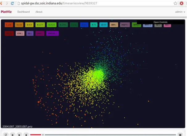
[image:5.612.155.458.428.649.2]We have developed a web browser based 3D visualization tool called WebPlotViz[8] for time series data visualization. The tool uses three.js JavaScript library for rendering 3D plots in the browser. The tool can be used to visualize sequence of time series 3D data using its play function. The 3D point files along with the metadata are stored in NoSQL databases and allows scalable plot data processing in the back end. The user can use the mouse to rotate the plots and zoom in and out of plots. Also the user can assign colors and special shapes to points for visualization. We chose categories to classify stocks which then show up colored differently in the visualization. In the next two subsections, we describe two ways we have used to classify stocks. Currently each visualization can examine one of these categorizations.
5.2 Classification by Industry Sectors
We classify stocks into sectors according to the NASDAQ industry classifications and color the points in 3D space by the sectors. We obtained the sectors from a REST API provided by NASDAQ for retrieving such information. The stocks are divided into 12 major industries including, Basic Industries, Capital Goods, Consumer Durables, Consumer Non-Durables, Consumer Services, Energy, Finance, Healthcare, Miscellaneous, Public Utility, Technology and Transportation. Some companies are not listed under any of the above industries. These major industries are further divided into sub-industries.
5.3 Classification by Stock Value Change
To visually see the distribution of stocks in the 3D space a histogram based coloring approach is used. Stocks are put into bins according to the relative change of prices of the corresponding time window. Then for each bin we assign a color and use that color to paint the stocks fall into that bin. A unified range across all the stocks are chosen by randomly picking a number of results from the set of windows we are interested in and getting the min and max change of these time windows across all the stocks. The first bin has a range starting from -Infinity and last bin has a range to +Infinity. The range of stock differences are varying widely and can be modeled as a normal distribution.
5.4 Special Symbols for Chosen Stocks
In the 3D plots we mark our special fiducial stocks and few stocks with large market capitalizations using special symbols (glyphs). These glyphs allow us to visualize them clearly in the plot and track their movements through time clearly. In future work we can allow more specific stocks to be tracked and also to study trajectory of individual securities.
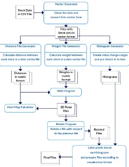
6 Data Processing Pipeline
We run all the steps including pre-processing, data analytics and post processing steps in a scripted workflow. For this application we primarily use MPI as the key technology and uses a HPC cluster to run the workflow. All the programs in the workflow are written using Java and the integration is achieved using bash scripts. The MDS and Levenberg-Marquardt Rotation algorithms are Java based MPI applications, running efficiently in parallel.
Preprocessing steps mainly focus on data cleansing and preparing the data to suite the inputs of the MDS algorithm. These data are run through the MDS algorithm to produce the 3D points. There are 523 data segments from 2004 to 2015 with a segmentation of 1 Year time window and 7 day shifts. For each of these data segment we first put the stocks into vector form. For each vector file we created, a distance matrix file and weight file is being calculated according to equations explained in section 3.2 and 3.3. At the next step these files are being used as inputs to each MDS run. For this set we run MDS for each distance file with 96 MPI ranks on 4 nodes, which typically completes in 3 ~ 4 minutes. MDS runs are done in parallel because there is no dependency between the MDS runs.
Each MDS Projection is ambiguous to rotations, reflections and translation, which was addressed by a least squares fit described in Sec. 4.3. To find the best transformation between all consecutive pairs of projections. After the 3D points are generated by MDS for each data segment we transform these points so that they can be visualized as a time series. Because two consecutive data segments can have different set of points, we find the transformation with respect to the common points between the two consecutive segments. After the transformation is found, we apply this transformation to the rest of the points not in the common set. Even Though the transformation program can be run in parallel by distributing the points of a single rotation into multiple MPI ranks, it cannot be run in parallel for different data segments because we are depending on the previous data segment’s transformation to do the next transformation.
Figure 2 Data processing pipeline of the application
7 Results & Discussion
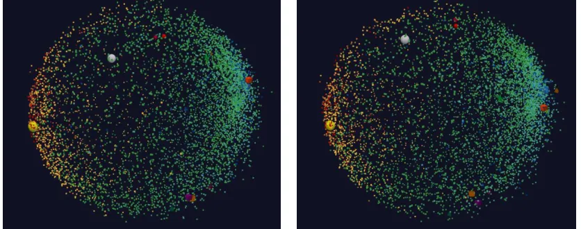
Few plots we obtained using the dataset are shown in Figure 3, 4 and 5. The glyphs shows the reference stocks. The different colors are using the histogram coloring approach. In Figure 3 we show few consecutive plots from the time series. Figure 4 shows the plots with L = 1 for equation 3 and figure 5 shows the plots for L calculated according to equation 4. As expected the shapes of the plots are different.
[image:7.612.68.554.536.619.2]Figure 4 A two random sample plots from the 2004 to 2015 time series for distance formula with L = 1 and labeled by histogram
Figure 5 A two random sample plots from the 2004 to 2015 time series for distance formula with L = log ratio and labeled by histogram
The accuracy of the MDS projection of stocks to 3D is primarily visualized using the heat maps. Fig 6 is a sample heat map between 3D points and original distances for L=1 and Fig 7 is a heat map for L calculated using equation 4 case. It is evident from these heat maps that the majority of 3D projections are accurate. When majority of the 3D projections are accurate they create a dense area along the diagonal of the heat map plot; which can be seen as the dark colors along the diagonal of Fig 6 and 7.
Figure 7 The distance distribution of stocks and heat map between original distances vs 3D distances for L = log ratio
The chi square error of the optimization to match one plot to the next plot is shown in Fig. 8 for L = 1 case and in Fig. 9 for L as described in equation 4. These plots shows the individual errors for the sequence of transformations we have done for the data set of 2004 to 2015. The same information is captured as histograms of error in Fig. 10 and 11. We have seen high error values in some cases even though their frequency is less. Because consequent segments of stock data are different from each other we don't expect a perfect matching between the consequent 3D points and we believe these high errors are due to turbulence in the stock market.
[image:9.612.102.512.333.457.2]Figure 8 Transformation error for consecutive data segments from 2004 to 2015 for distance formula with L = 1
Figure 9 Transformation error for consecutive data segments from 2004 to 2015 for distance formula with L = log ratio
0 10 20 30 40 50
Figure 10 Histogram of transformation error for distance formula with L = 1
Figure 11 Histogram of transformation error for distance formula with L = log ratio
All the time series plots are publicly available in the WebPlotViz tool hosted at the address http://spidal-gw.dsc.soic.indiana.edu/.
8 Conclusions & Future Work
We discussed our initial results of applying Multidimensional Scaling to financial data to visualize the changes of stocks over time. Our methods are scalable both in number of stocks and number of data segments considered. We are extending our approach into different distance metrics as well as data segmentations obtain deeper understanding about the financial data. We are planning to extend the system using big data technologies to efficiently manage large amounts of data required at various steps of the workflow. This will allow real time interactive visualization of the market structure with user customization. Another interesting technology improvement is handling of real-time stock data and using the faster interpolative MDS and rotation technologies for updating quickly structure maps.
9 Acknowledgements
This work is partially supported by NSF 1443054 grant as it used data analytics from the SPIDAL library. Further we would like to extend our gratitude to FutureSystems team for their support with the computational infrastructure. We thank Linda Hatden at Elizabeth City State University for the support for the summer REU contributions of Maya Smith and Anthony Scott.
References
[1]
(2015, November 22, 2015).
Three.js Revision 73
. Available:
http://threejs.org/
[2]
Y. Ruan, "Scalable and robust clustering and visualization for large-scale bioinformatics data," Indiana
University, 2014.
254
145
39
20 10 17 6 5 6 3 3 0 1 1 2 2 3 3 0 1 1
2 4 6 8 10 12 14 16 18 20 22 24 26 28 30 32 34 36 38 40 42
0 10 195
177
67 35
11 9 5 7 2 1 1 0 1 1
[image:10.612.198.416.226.385.2]