Machine learning for performance enhancement of molecular dynamics simulations

of molecular dynamics simulations

JCS Kadupitiya1_{, Geoffrey C. Fox}1_{, and Vikram Jadhao}1[0000−0002−8034−2654]

Intelligent Systems Engineering, Indiana University, Bloomington IN 47408, USA

{kadu,gcf,vjadhao}@iu.edu

Abstract. We explore the idea of integrating machine learning with simulations to enhance the performance of the simulation and improve its usability for research and education. The idea is illustrated using hy-brid openMP/MPI parallelized molecular dynamics simulations designed to extract the distribution of ions in nanoconfinement. We find that an artificial neural network based regression model successfully learns the desired features associated with the output ionic density profiles and rapidly generates predictions that are in excellent agreement with the results from explicit molecular dynamics simulations. The results demon-strate that the performance gains of parallel computing can be further enhanced by using machine learning.

Keywords: Machine Learning·Molecular Dynamics Simulations· Par-allel Computing·Scientific Computing·Computational Clouds

1

Introduction

In the fields of physics, chemistry, bioengineering, and materials science, it is hard to overstate the importance of parallel computing techniques in provid-ing the needed performance enhancement to carry out long-time simulations of systems of many particles with complex interaction energies. These enhanced simulations have enabled the understanding of microscopic mechanisms under-lying the macroscopic material and biological phenomena. For example, in a typical molecular dynamics (MD) simulation of ions in nanoconfinement [2, 13] (Fig. 1),≈1 nanosecond of dynamics of≈500 ions on one processor takes≈12 hours of runtime, which is prohibitively large to extract converged results for ion distributions within reasonable time frame. Performing the same simulation on a single node with multiple cores using OpenMP shared memory reduces the runtime by a factor of 10 (≈1 hour), enabling simulations of the same system for longer physical times. Using MPI dramatically enhances the simulation perfor-mance: for systems with thousands of ions, speedup of over 100 can be achieved, enabling the generation of the needed data for evaluating converged ionic dis-tributions. Further, a hybrid OpenMP/MPI approach can provide even higher speedup of over 400 for similar-size systems enabling state-of-the-art research

?

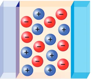
Fig. 1.Sketch of ions represented by blue and red spheres confined by material surfaces.

with simulations that can explore the dynamics of ions with less controlled ap-proximations, accurate potentials, and for tens or hundreds of nanoseconds over a wider range of physical parameters.

Despite the employment of the optimal parallelization model suited for the size and complexity of the system, scientific simulations remain time consuming. This is particularly evident in the area of using simulations in education where real-time simulation-driven responses to students in classroom settings are desir-able. While in research settings, instantaneous results are generally not expected and simulations can take up to several days, it is often desirable to rapidly ac-cess expected trends associated with relevant physical quantities that could have been learned from past simulations or could be predicted with reasonable accu-racy based on the history of data generated from earlier simulation runs. As an example, consider a simulation framework, Ions in Nanoconfinement, that we deployed as a web application on nanoHUB to execute the aforementioned simulations of ionic systems [14]. In classroom usage, we have observed that the fastest simulations can take about 10 minutes to provide the converged ionic densities while the slowest ones (typically associated with larger system sizes and more complex ion-ion interaction energies) can take over 3 hours. Similarly, for research applications, not having a rapid access to expected overall trends in the key simulation output quantities (e.g., the variation of contact density as a function of ion concentration) can make the process of starting new investi-gations unwieldy and time-consuming. Primary factors that contribute to this scenario are the time delays resulting from the combination of waiting time in a queue on a computing cluster and the actual runtime for the simulation.

regres-sion model, trained on data generated via these simulations, successfully learns pre-identified key features associated with the output ionic density profile (the contact, mid-point, and peak densities). The ML approach entirely bypasses simulations and generates predictions that are in excellent agreement with re-sults obtained from explicit MD simulations. The rere-sults demonstrate that the performance gains of parallel computing can be enhanced using data-driven ap-proaches such as ML which improves the usability of the simulation framework by enabling real-time engagement and anytime access.

2

Background and Related Work

2.1 Coarse-grained simulations of ions in nanoconfinement

The distribution of ions often determines the assembly behavior of charged or neutral nanomaterials such as nanoparticles, colloids, or biological macro-molecules. Accurate knowledge of this ionic structure is exploited in many ap-plications [8] including the design of double-layer supercapacitor and the extrac-tion of metal ions from wastewater. As a result, extracting the distribuextrac-tion of ions in nanoconfinement created by material surfaces has been the focus of re-cent experiments and computational studies [18, 22, 24, 21, 13]. From a modeling standpoint, the surfaces are often treated as planar interfaces considering the size difference between the ions and the confining material particles, and the solvent is coarse-grained to speed-up the simulations. Such coarse-grained simu-lations have been employed to extract the ionic distributions over a wide range of electrolyte concentrations, ion valencies, and interfacial separations using codes developed in individual research groups [2, 3, 13] or using general purpose soft-ware packages such as ESPRESSO [16] and LAMMPS [19].

Generally, the average equilibrium ionic distribution, resulting from the com-peting inter-ionic steric and electrostatic interactions as well as the interactions between the ions and surfaces, is a quantity of interest. However, in many cases, the density of ions at the point of closest approach of the ion to the interface (contact density), the peak density, or the density at the center of the slit (mid-point density) directly relate to important experimentally-measurable quantities such as the effective force between the confining surfaces or the osmotic pres-sure [24, 21]. It is thus useful to compute the variation of the contact, peak, and mid-point densities as a function of the solution conditions or ionic attributes.

2.2 Machine learning for enhancing simulation performance

for nuclei-electron systems by learning the selection of probable configurations in MD simulations, which enabled bypassing explicit simulations for several steps. The integration of ML layer for performance enhancement of scientific sim-ulation frameworks deployed as web applications is relatively far less explored. nanoHUB is the largest online resource for education and research in nanotech-nology [15]. This cyberinfrastructure hosts over 500 simulation tools and serves 1.4 million users worldwide. Our survey indicated that only one simulation tool on nanoHUB [10] employs ML-based methods to enhance the performance and usability of the simulation software. This simulation tool employs a deep neural network to bypass computational limitations in extracting transfer times asso-ciated with the excitation energy transport in light-harvesting systems [10].

3

Framework for Simulating Ions in Nanoconfinement

We developed a framework for simulating ions in nanoscale confinement (referred here as the nanoconfinement framework) that enabled a systematic investigation of the self-assembly of ions characterized by different ionic attributes (e.g., ion valency) and solution conditions (e.g., ion concentration and inter-surface sepa-ration) [11, 13, 14]. The framework has been employed to extract the ionic struc-ture in electrolyte solutions confined by planar and spherical surfaces. Results have elucidated the microscopic mechanisms involving the ionic correlations and steric effects that determine the distribution of ions [11–13].

In the work presented here, we focus on ions confined by unpolarizable sur-faces where the simulations are relatively faster [13], thus easing the training and testing of the ML model. We identify the following system attributes as key parameters that determine the self-assembly of ions: inter-surface separation or confinement lengthh, ion valencies (zp,zn associated with the positive and

neg-ative ions), electrolyte concentrationc, and ion diameterd. We ignore the effects arising due to the solvent-induced asymmetry in ionic sizes, and assign the pos-itive and negative ions with the same diameter. Additional details regarding the model and simulation method can be found in the original paper [13].

The nanoconfinement framework employs a customized code, written in C++ programming language, for simulating ions near unpolarizable interfaces. The code, freely available as an open-source repository on GitHub [14], is accelerated using a hybrid parallel programming technique (see Sec. 3.1). This framework is also deployed as a web application (Ions in Nanoconfinement) on nanoHUB [14] (see Sec. 3.2). We have verified that the ionic density profiles obtained using our in-house developed code agree with the densities extracted via simulations performed in LAMMPS. We note that the ML model explored in the following sections to predict the desired key ionic densities is agnostic to the particular code engine that enables the MD simulations for generating the training dataset.

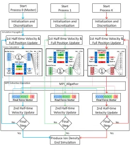
3.1 Hybrid OpenMP/MPI parallelization

Fig. 2. Hybrid model implemented in the Force Calculation block using MPI and OpenMP to accelerate the nanoconfinement framework.

First, the velocities of all ions is updated for half timestep∆/2, following which the positions of all ions are updated for∆. At this point, the forces on all ions are computed, and finally the velocities for all ions are updated for the next

∆/2. Once the system reaches equilibrium, the positions of the ions are stored periodically to extract density profiles.

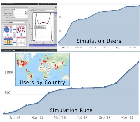
Fig. 3.A screenshot of the GUI (top left) and usage statistics of the nanoconfinement framework deployed on nanoHUB.

the maximum access locality, a minimum of cache misses, non-uniform memory access (NUMA) traffic and inter-node communication [20].

3.2 Deployment on nanoHUB cloud

The nanoconfinement framework is deployed as a web application (Ions in Nanocon-finement) [14] on the nanoHUB cloud cyberinfrastructure. nanoHUB provides a user-friendly, web-based access for executing simulation codes to researchers, students, and educators broadly interested in nanoscale engineering [15]. In less than 1 year of its launch, the Ions in Nanoconfinement application has nucle-ated 58 users worldwide and has been run over 1200 times [14]. This application is designed to launch simulations that use virtual machines or supercomputing clusters depending on user-selected inputs, and it has been employed to teach graduate courses at Indiana University. Advances in the framework that enable real-time results can significantly enhance the user-experience of the commu-nity that employs this application in both education and research. The current version of “Ions in Nanoconfinement”, like almost all other applications on the nanoHUB platform, does not support this feature.

4

ML-enabled Performance Enhancement

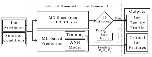
Fig. 4.System overview of the enhanced nanoconfinement framework.

framework. These inputs are used to launch the MD simulation on the high-performance computing (HPC) cluster. Simultaneously, these inputs are also fed to the ML-based density prediction module to predict the contact, mid-point, and peak densities. The outputs of the MD simulation are the ion density profiles that characterize the ionic structure near unpolarizable interfaces. Error handler aborts the program and displays appropriate error messages when a simulation fails due to any pre-defined criteria. In addition, at the end of the simulation run, ionic density values are saved for future retraining of the ML model. For every 2500 new simulation runs, ML model is retrained.

After reviewing and experimenting with many ML techniques for parameter tuning and prediction including polynomial regression, support vector regres-sion, decision tree regresregres-sion, and random forest regresregres-sion, the artificial neural network (ANN) was adopted for predicting critical features associated with the output ionic density. Figure 5 shows the details of this ANN-based ML model. The data preparation and preprocessing techniques, feature extraction and re-gression techniques as well as their validation are discussed below.

4.1 Data preparation and preprocessing

Prior domain experience and backward elimination using the adjusted R squared is used for creating the training data set. Five input parameters that significantly affect the dynamics of the system are identified: confinement length h, positive valency zp, negative valency zn, salt concentration c, and the diameter of the

ions d. Future work will explore the training with additional input parameters such as temperature and solvent permittivity that are fixed in this initial study to room temperature (298 K) and water permittivity (≈80) respectively.

Contact densityρc, mid-point (center of the slit) densityρm, and peak density ρp associated with the final (converged) distribution for positive ions were

Fig. 5.ANN-based regression model to enhance the nanoconfinement framework.

h ∈ (3.0,4.0) nm, zp ∈ 1,2,3 (in units of electronic charge |e|); zn ∈ −1,−2

(in units of |e|); c ∈(0.3,0.9) M, and d∈ (0.5,0.75) nm. All simulations were performed for over ≈ 5 nanoseconds. The entire data set was separated into training and testing sets using a ratio of 0.7:0.3. Min−max normalization filter was applied to normalize the input data at the preprocessing stage.

4.2 Feature extraction and regression

The ANN algorithm with two hidden layers (Fig. 5) was implemented in Python for regression of three continuous variables in the ML model. Outputs of the hidden layers were wrapped with the relu function; the latter was found to converge faster compared to the sigmoid function. No wrapping functions were used in the output layers of the algorithm as ANN was trained for regression.

By performing a grid search, hyper-parameters such as the number of first hidden layer units, second hidden layer units, batch size, and number of epochs were optimized to 17, 9, 25, and 100 respectively. Adam optimizer was used as the back propagation algorithm. The weights in the hidden layers and in the output layer were initialized to random values using a normal distribution at the beginning. The mean square loss function was used for error calculation. To stop overtraining the network, a drop out mechanism for hidden layer neurons was employed during the training time. ANN implementation, training, and testing was programmed with the aid of keras and sklearn ML libraries [7, 5, 1].

5

Results

5.1 Bypassing simulations with ML-enabled predictions

0 0.2 0.4 0.6 0.8 1 1.2

0 0.2 0.4 0.6 0.8 1 1.2

Contact Density from ML (M)

Contact Density from MD (M)

MD ML

0 0.5 1 1.5 2 2.5

0 0.5 1 1.5 2 2.5

Peak Density (ML)

Peak Density (MD)

0 0.2 0.4 0.6 0.8 1 1.2

0 0.2 0.4 0.6 0.8 1 1.2

Center Density (ML)

Center Density (MD)

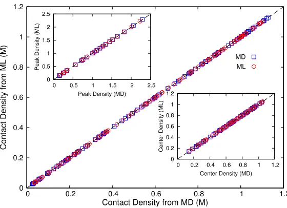
Fig. 6.Accuracy comparison between ML predictions (red circles) and MD simulation results (blue squares) for the contact densities associated with the distribution of ions in systems characterized by input parameters: h ∈ (3.0,4.0) nm, zp ∈ 1,2,3, zn ∈ −1,−2,c∈(0.3,0.9) M, andd∈(0.5,0.75) nm. Top-left and bottom-right insets show, respectively, the comparison for the peak and mid-point densities for the same systems.

mid-point density (ρm), and peak density (ρp). These models were tested on 2060

sets of input parameters (h, zp, zn, c, d). These sets were comprised of parameter

values within the range for which the models were trained; see Section 4.1. Table 1 shows the success rate and the mean square error (MSE) for testing data sets. Success rate was calculated based on the error bars (standard deviation) associated with the density values obtained via MD simulations: ML prediction was considered successful when the predicted density value was within the error bar of the simulation estimate. Simulations were run for sufficiently long times (over ≈ 5 nanoseconds) to obtain converged density estimates and error bars.

Table 1.Comparison of regression models for the prediction of output density values.

Model Contact Density Midpoint Density Peak Density

0.06 0.08 0.1 0.12 0.14 0.16 0.18 0.2

0.5 0.55 0.6 0.65 0.7 0.75

Contact Density (M)

Ion diameter d (nanometers) ML

MD

0.205 0.210 0.215 0.220 0.225

3 3.2 3.4 3.6 3.8 4

Contact Density (M)

Confinement Length h (nanometers)

ML MD

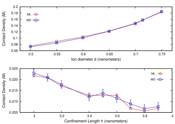
Fig. 7.(Top) Trendlines for contact density vs. ion diameter for systems with h= 4 nm, zp = 3, zn = −1, andc = 0.85 M. (Bottom) Trendlines for contact density vs. confinement length for systems withzp= 2,zn=−1,c= 0.9 M, andd= 0.553 nm.

Reported MSE values are calculated using k-fold cross-validation techniques with k = 20. ANN based regression model predicted ρc, ρm and ρp accurately with

a success rate of 95.52% (MSE≈0.0000718), 92.07% (MSE≈0.0002293), and 94.78% (MSE≈0.0002306) respectively. ANN outperformed all other non-linear regression models as evident from Table 1.

Figure 6 shows the comparison between the predictions made by the ML model and the results obtained from MD simulations for the contact, mid-point, and peak densities associated with positive ions. For clarity, results are shown for a randomly selected subset of the entire testing dataset described in Section 4.1.

ρc,ρmandρppredicted by the ML model were found to be in excellent agreement

with those calculated using the MD method; data from either approach falls on the dashed line which indicates linear correlation.

5.2 Rapid access to trendlines using ML

Trendlines exhibiting the variation ofρc,ρm, andρp for a wide range and

com-binations of the five input parameters (h, zp, zn,c, d) were extracted using the

ML model. In Figures 7 and 8, we show a small selected subset of these trends. Figure 7 shows the variation of the contact densityρcwith the ion diameter d and confinement length h. Figure 7 (top) illustrates how ρc varies with d ∈

(0.5,0.75) nm at constanth= 4 nm,zp = 3,zn=−1, andc= 0.85 M. Figure 7

0.5 1 1.5 2 2.5

0.3 0.4 0.5 0.6 0.7 0.8 0.9

Density (M)

Salt Concentration c (M)

Contact, ML

Contact, MD

Center, ML

Center, MD

Peak, ML

Peak, MD

Fig. 8.Contact, peak, and center-of-the-slit (mid-point) density vs. salt concentration associated with the distribution of ions for systems characterized with h = 3.2 nm,

zp= 1,zn =−1, and d= 0.714 nm. Closed symbols represents ML predictions and open symbols with error bars are MD simulation results.

between 3.0 and 4.0 nm, with other parameters held constant (zp= 2,zn=−1, c = 0.9 M, and d= 0.553 nm). Circles represent ML predictions and squares show MD results. ML predictions are within the errorbars generated via MD simulations and follow the simulation-predicted trends for both cases. Results demonstrate that contact density varies rapidly when the diameter is changed but exhibits a slower variation when the confinement length is varied. We find that the same ML model is able to track the distinct variations while exhibiting different resolution (sensitivity) criteria.

Figure 8 shows similar comparison between ML and MD results for the varia-tion ofρc,ρmandρpvs. salt concentrationc. Excellent agreement is seen between

the two approaches. We note that the prediction time for the ML model to ob-tain these densities is in the order of a few seconds while the simulations can take up to hours to compute one contact density with similar accuracy level.

5.3 Speedup

Traditional speedup formulae associated with parallel computing methods need to be adapted for evaluating the speedup associated with the ML-enhanced sim-ulations. We propose the following simple formula which is illustrative at this preliminary stage. We define the ML speedup as:

S = tsim

tp+ttr·Ntr/Np

, (1)

wheretsim is the time to run the MD simulation via the sequential model,tp is

or “lookup” time) for one set of inputs, Np is the number of predictions made

using the ML model,Ntr is the number of elements in the training dataset, and ttr is the average walltime associated with the MD simulation to create one of

these elements. Ntrttr represents the total time it took to create the training

dataset which includes the generation of the training data using MD simulations and the tensorflow training time.

The above formula highlights the key feature of the ML-based approach: the speedupS increases as ML model is used to make more predictions, that is,S

rises with increasing Np. As Np approaches infinity, S approachestsim/tp; for

our MD simulations (tsim ≈12 hours) and ANN model (tp≈0.25 seconds), we

find this ratio to be over 105_{. On the other hand, if the number of predictions} made through the ML model is small (smaller Np), then S is expected to be

small. We explore this scenario further. For implementing our ML model, the training dataset consisted of 4760 simulation configurations, makingNtr= 4760.

The timettrto generate one element of this training set is similar to the average

runtime of the parallelized MD simulation; we find ttr ≈tsim/100. Using these

relations and notingtptsim, a lower bound on speedup can be derived as the

result forNp= 1. For this case, we find the “speedup”S ≈tsim/(ttrNtr)≈10−2.

Finally, when the number of predictionsNpare similar to the number of elements

in the training dataset Ntr, then Eq. 1 yieldsS ≈tsim/ttr, which is equivalent

to the speedup associated with the traditional parallel computing approach.

6

Outlook and Future Work

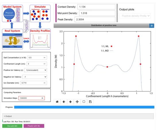
Based on the aforementioned investigations, we propose to design and integrate an ML layer with the nanoconfinement framework. This enhanced application will be deployed on nanoHUB using the Jupyter python notebook interface. Fig. 9 shows a sketch of the proposed GUI. Users will be able to click on both “Run with MD” button as well as “Predict with ML” button simultaneously or separately depending on the desired information. “Predict with ML” button will activate the ML layer and predict ρc, ρm, and ρp almost instantaneously.

These ML predicted values will be shown in three text boxes and will appear as markers on the density profile plot. If users also select “Run with MD”, the entire density profile will be added at the end of the simulation. For illustration purposes, the final density plot using this integrated MD + ML approach for the input parametersh= 3.0 nm;zp= 1,zn =−1,c= 0.9 M, andd= 0.714 nm is

shown in Fig. 9.

simula-Fig. 9.Proposed GUI for integrating an ML layer with the nanoconfinement framework deployed on nanoHUB. The GUI includes text boxes (top) showing the contact, mid-point, and peak densities for a representative ionic system. These results also appear as markers on the plot (right) along with the MD generated density profile.

tions are used in research and education. We expect that the usefulness of the ML-enabled enhancements demonstrated in this work strengthen the case for modern scientific simulation applications to be designed and developed with an ML wrapper that both optimizes the application execution and learns from the explicit simulations.

References

1. Abadi, M., Barham, P., Chen, J., Chen, Z., Davis, A., Dean, J., Devin, M., Ghe-mawat, S., Irving, G., Isard, M., et al.: Tensorflow: a system for large-scale machine learning. In: OSDI. vol. 16, pp. 265–283 (2016)

2. Allen, R., Hansen, J.P., Melchionna, S.: Electrostatic potential inside ionic solu-tions confined by dielectrics: a variational approach. Phys. Chem. Chem. Phys.3, 4177–4186 (2001)

3. Boda, D., Gillespie, D., Nonner, W., Henderson, D., Eisenberg, B.: Computing induced charges in inhomogeneous dielectric media: Application in a monte carlo simulation of complex ionic systems. Phys. Rev. E69(4), 046702 (Apr 2004) 4. Botu, V., Ramprasad, R.: Adaptive machine learning framework to accelerate ab

initio molecular dynamics. International Journal of Quantum Chemistry115(16), 1074–1083 (2015)

6. Butler, K.T., Davies, D.W., Cartwright, H., Isayev, O., Walsh, A.: Machine learning for molecular and materials science. Nature559(7715), 547 (2018)

7. Chollet, F., et al.: Keras (2015)

8. Feng, G., Qiao, R., Huang, J., Sumpter, B.G., Meunier, V.: Ion distribution in electrified micropores and its role in the anomalous enhancement of capacitance. ACS Nano4(4), 2382–2390 (2010)

9. Ferguson, A.L.: Machine learning and data science in soft materials engineering. Journal of Physics: Condensed Matter30(4), 043002 (2017)

10. H¨ase, F., Kreisbeck, C., Aspuru-Guzik, A.: Machine learning for quantum dynam-ics: deep learning of excitation energy transfer properties. Chemical science8(12), 8419–8426 (2017)

11. Jadhao, V., Solis, F.J., Olvera de la Cruz, M.: Simulation of charged systems in heterogeneous dielectric media via a true energy functional. Phys. Rev. Lett.109, 223905 (Nov 2012)

12. Jadhao, V., Solis, F.J., Olvera de la Cruz, M.: A variational formulation of elec-trostatics in a medium with spatially varying dielectric permittivity. The Journal of Chemical Physics138(5), 054119 (2013)

13. Jing, Y., Jadhao, V., Zwanikken, J.W., Olvera de la Cruz, M.: Ionic structure in liquids confined by dielectric interfaces. The Journal of chemical physics143(19), 194508 (2015)

14. Kadupitiya, K., Marru, S., Fox, G.C., Jadhao, V.: Ions in nanoconfinement (Dec 2017), https://nanohub.org/resources/nanoconfinement, online on nanoHUB; source code on GitHub at github.com/softmaterialslab/nanoconfinement-md 15. Klimeck, G., McLennan, M., Brophy, S.P., III, G.B.A., Lundstrom, M.S.:

nanohub.org: Advancing education and research in nanotechnology. Computing in Science Engineering10(5), 17–23 (Sept 2008)

16. Limbach, H.J., Arnold, A., Mann, B.A., Holm, C.: ESPResSo – an extensible sim-ulation package for research on soft matter systems. Comp. Phys. Comm.174(9), 704–727 (May 2006)

17. Liu, J., Qi, Y., Meng, Z.Y., Fu, L.: Self-learning monte carlo method. Phys. Rev. B95, 041101 (Jan 2017)

18. Luo, G., Malkova, S., Yoon, J., Schultz, D.G., Lin, B., Meron, M., Benjamin, I., Vansek, P., Schlossman, M.L.: Ion distributions near a liquid-liquid interface. Science311(5758), 216–218 (2006)

19. Plimpton, S.: Fast parallel algorithms for short-range molecular dynamics. Journal of Computational Physics117(1), 1 – 19 (1995)

20. Rabenseifner, R., Hager, G., Jost, G.: Hybrid mpi/openmp parallel programming on clusters of multi-core smp nodes. In: 2009 17th Euromicro International Con-ference on Parallel, Distributed and Network-based Processing. pp. 427–436. IEEE (2009)

21. dos Santos, A.P., Netz, R.R.: Dielectric boundary effects on the interaction between planar charged surfaces with counterions only. The Journal of chemical physics

148(16), 164103 (2018)

22. Smith, A.M., Lee, A.A., Perkin, S.: The electrostatic screening length in concen-trated electrolytes increases with concentration. The journal of physical chemistry letters7(12), 2157–2163 (2016)

23. Spellings, M., Glotzer, S.C.: Machine learning for crystal identification and discov-ery. AIChE Journal64(6), 2198–2206 (2018)

24. Zwanikken, J.W., Olvera de la Cruz, M.: Tunable soft structure in charged fluids confined by dielectric interfaces. Proceedings of the National Academy of Sciences